Abstract
This paper creates a global similarity network between city-level dialects of English in order to determine whether external factors like the amount of population contact or language contact influence dialect similarity. While previous computational work has focused on external influences that contribute to phonological or lexical similarity, this paper focuses on grammatical variation as operationalized in computational construction grammar. Social media data was used to create comparable English corpora from 256 cities across 13 countries. Each sample is represented using the type frequency of various constructions. These frequency representations are then used to calculate pairwise similarities between city-level dialects; a prediction-based evaluation shows that these similarity values are highly accurate. Linguistic similarity is then compared with four external factors: (i) the amount of air travel between cities, a proxy for population contact, (ii) the difference in the linguistic landscapes of each city, a proxy for language contact, (iii) the geographic distance between cities, and (iv) the presence of political boundaries separating cities. The results show that, while all these factors are significant, the best model relies on language contact and geographic distance.
1. Introduction
Recent work in construction-based dialectology has shown that syntactic variation across geographic dialects is both (i) remarkably robust, which creates highly accurate models that capture variation across many constructions (, , ), and (ii) remarkably stable, which create models that remain accurate over time and register (; ; ). This line of work has, however, remained focused on modeling patterns of variation rather than the sources of variation. Moving beyond such descriptions, we interrogate what lexico-grammatical mechanisms of language change have led to the current distribution of grammatical variants that we observe. While computational methods allow observations at a much larger scale across both population size and coverage of the grammar, this expanded scale has not yet been leveraged for testing the influence of external factors. Meanwhile, computational work which has focused on this question (; ; ) has relied on data from linguistic atlases, establishing the foundation for this type of experiment while remaining difficult to scale.
The current paper addresses this gap by examining the influence that four external factors have on the grammatical similarity between dialects: First, we consider language contact, a product of the mix of languages present in a local dialect area; this is operationalized using geo-referenced corpora to estimate what languages are used digitally in each area, in what might be called the linguistic landscape ().1 Second, we consider population contact, or the amount of mutual exposure between two dialect areas; this is operationalized using estimates of air travel (). Third and fourth, we use geographic distance and political boundaries as additional factors which could influence dialect similarity. The basic idea is to determine the degree to which these representations of linguistic and social interactions within and between dialect areas can be used to predict the synchronic patterns of dialect similarity. This work is made possible by computational methods which allow us to observe pairwise similarities between 256 city-level dialects of English.
We approach computational dialectology from a constructional perspective by observing the variation across many parts of the grammar rather than within isolated features (). This is an important perspective for two reasons: First, because language is a complex system (), this means, for example, that small changes in one part of the grammar may produce large changes in another part of the grammar (; ). Second, if the grammar is structured as a network (), we would expect that processes of diffusion unfold uniquely in different parts of the grammar. This implies that similarity between dialects within one portion of the grammar does not equal general similarity across all portions.
In order to deal with the grammar as a complex network, we use computational construction grammar working with approximately 15,000 constructions. In Section 3.2, we describe the nature of these constructions, and in Section 3.3, we evaluate their ability to measure dialect similarity. In particular, we conduct an accuracy evaluation to determine whether this operationalization of construction-based similarity is able to predict which cities fall within the same political boundaries, by taking that accuracy as a measure for validating the overall quality of the similarity measures themselves. As shown later, the measures make highly accurate predictions about political boundaries.
Our first hypothesis is that language contact will cause dialects with more similar linguistic environments to themselves become more similar. For instance, we expect that two varieties of English that co-occur with the same non-English languages will have more similar grammars. This hypothesis concerns interactions between languages within a dialect area. We operationalize language contact by first quantifying the linguistic landscape of each city and then comparing how similar this landscape is between pairs of cities. This is explored further in Section 3.4 as illustrated in Table 5.
Our second hypothesis is that population contact will also cause dialects with more connected populations to have more similar grammars as a result of mutual exposure. For instance, we expect that cities with more air travel between them reflect cities whose populations have had a greater degree of contact. This hypothesis concerns interactions between dialect areas. This is also discussed in Section 3.4.
Our third hypothesis is that the geographic distance between cities will have a further influence on the similarity between city-level dialects. Because we use the identification of political boundaries as a validation measure, we do not use this information in later experiments. The larger goal of these experiments is to quantify how much of the observed patterns of similarity can be predicted given these factors of language contact and population contact and geographic distance between cities. The contribution of this paper is, first, to focus on grammatical similarity and, second, to expand the scale of these experiments by eliminating the dependence on data from a linguistic atlas.
The experiments use digital corpora from social media (tweets) in English from 256 local urban areas in 13 countries, all representing either inner-circle or outer-circle varieties. These tweets are aggregated into samples of approximately 3900 words each. These aggregated samples control for variations in topic and/or register by selecting one message each for 250 non-functional keywords like season or wish. This ensures that each sample from each dialect area represents the same mix of topics (keywords) from the same register (social media). The total corpus contains 46,228 samples or approximately 180 million words. Further details about the data are discussed below in Section 3.1.
The grammatical structure of each sample is quantified using the type frequency of constructions, drawing on work in computational construction grammar (). These unsupervised grammars are especially useful for observing the variation because (i) they can be learned specifically from data representing diverse dialects and (ii) they capture variation across different levels of abstraction. In practical terms, this means that each sample is represented using the type frequencies of each construction in the grammar, thus focusing on the relative productivity of each construction. The similarity of two dialects is then quantified by comparing the observed frequencies using measures of similarity from forensic linguistics (). Two dialects are considered more similar when they have similar rates of construction productivity.
In these experiments, the grammatical similarity between dialects provides a dense network of over 32,000 similarity values. We use this network to describe grammatical variation in English. Our hypothesis is that this similarity network can be explained or predicted to a large degree by (i) information about language contact in each local area and (ii) information about the amount of population contact between local areas. We also include information about (iii) geographic distance. Importantly, this question could not be investigated at the necessary scale without a reliance on computational methods because no linguistic atlas, for instance, contains a sufficient number of global cities to adequately represent English dialects.
The Section 2 focuses on related work in corpus-based and computational dialectology. The Section 3 provides a description of the corpus data, a description of computational construction grammar as an operationalization of grammatical features and how we calculate the similarity of city-level dialects, and a description of how we operationalize factors like population contact and language contact. The Section 4 undertakes a regression-based analysis and a clustering analysis to determine which factors are most connected with the grammatical similarity of dialects. And, finally, the Section 5 considers what these results tell us about the sources of grammatical variation. The final conclusion is that, while all factors have some influence, language contact is more important than population contact in predicting the grammatical similarity between dialects.
2. Related Work
This study is situated in a tradition of dialectometry which relies on geo-referenced corpora (; ; ). While early computational work was based on dialect surveys (; ; , ), the field shifted to a focus on corpus data as digital corpora became more widely available (, ; ; , ). In this paradigm, the starting point is production data (i.e., written corpora) collected from known populations (i.e., specific geographic locations). Social media, in particular, became a primary source of data, with a dominant focus on lexical variation (; ; ; ; ; ), including lexical variation at the level of senses (). Given the reliance on written corpora, morphosyntactic variation became increasingly important (), sometimes with small numbers of discrete variables (; , ; ) and then with larger numbers of surface-level alternations ().
Taking seriously the view that the grammar is a complex system, work within construction grammar (often referred to as CxG) instead focused on variation across many constructional features (, , , ; ). These approaches include large numbers of features, requiring high-dimensional models like classifiers. In this paradigm, the modeling task is to distinguish between dialects: the best model of a dialect would thus be capable of distinguishing it from all other dialects. On a technical level, this is connected with work in natural language processing (NLP) which is concerned only with the problem of distinguishing between dialects, rather than studying dialectal variation itself (; ; ; ; ; ). While having a different theoretical aim, this work from NLP provides numerous technical advantages for the study of large-scale variation across dialects.
Previous work has also focused on constructional variation and change (), for example, by focusing on the combination of frequency and schematicity as factors in language change (; ). Because usage-based linguistics views language as an emergent system that ultimately derives from exposure, there has been a focus on differences in linguistic experience, even at the level of individuals (; ; ). And, because the grammar is viewed as a network, previous work has also examined variation within different strata of the grammar (; ). Viewed from this historical perspective, the contribution of this current study is to examine the impact that external variables like population contact have on dialectal similarity networks derived from high-dimensional constructional features that represent the grammar as a complex system. The impact of this work is to use large-scale computational experiments to test hypotheses about the sources of dialectal variation from a usage-based perspective, going beyond the modeling of patterns of variation to modeling sources of variation.
Previous work in dialectometry has also investigated the role of external factors for predicting dialect similarity. Earlier computational work investigated the relationship between linguistic distance (based on word-level phonology) and geographic distance, in order to understand the impacts of borders on dialects (). Other work used travel time as a measure to better understand the relationship between geographic and linguistic distance, as a measure which accounts for geographic barriers (). Travel time was quite explanatory in some countries (Norway), but less so in others (The Netherlands). Moving from phonological to lexical features, more recent work investigated the impact of physical geography, religious groups, and political boundaries on the similarity of Tuscan dialects (). Interestingly, this work found an interaction between the semantic domain and which external factor exerted the most influence. From the perspective of language as a complex system, this illustrates the importance of taking a broader view across both features subject to variation and the factors causing variation. This current work expands these earlier studies to syntactic features.
3. Materials and Methods
3.1. Corpus Data
This study relies on the written digital production collected from tweets. The use of written production data to study dialectal variation is motivated both by work which investigates the relationship between variation in written and in spoken registers () and also by work which investigates the impact of exposure to written language on language change (). These tweets are drawn from the Corpus of Global Language Use (cglu) (, ). Corpora representing individual cities are created by aggregating tweets into larger samples. The social media portion of the cglu contains publicly accessible tweets collected from 10,000 cities around the world, where each city is a point with a 25 km collection radius. Here the number of cities is reduced to those with a sufficient amount of data (at least 25 samples, aggregated as described below) from either inner-circle or outer-circle countries (). This paper works only with English-language corpora; tweets are tagged for language using both the idNet model () and the PacificLID model (); only tweets which both models predict to be English are included. An overview of this dataset is shown in Table 1.

Table 1.
Distribution of sub-corpora by region. Each sample is a unique sub-corpus with the same distribution of keywords, each approximately 3900 words in length.
A list of each city by country is available in Table A1 for inner-circle countries and in Table A2 for outer-circle countries, in Appendix A. Our goal is to create comparable corpora representing each local population using geo-referenced tweets. The challenge is that social media data represents many topics and sub-registers, so that there is a possible confound presented by geographically structured variations in the topic or sub-register. For instance, if tweets from Chicago are sports-related and tweets from Christchurch are business-related, then the observed variation is likely to be partially register-based as well as dialect-based. To control for the topic, we create samples by aggregating tweets which contain the same set of keywords. First, we select 250 common words which are neither purely topical nor purely functional: for example, girl, know, music, and project. These keywords are available in Table A3 in Appendix B. Second, for each local metro area, we create samples containing one tweet for each keyword; each sample thus contains 250 individual tweets, for a total size of approximately 3900 words. Importantly, the distribution of keywords is uniform across all samples from all local areas. This allows us to control for variations in a topic or sub-register which might otherwise lead to non-dialectal sources of variation. This corpus has been previously used for other studies of linguistic variation (; ).
To ensure a robust estimate of construction usage in each city, we only include those with at least 25 unique samples (thus, a total corpus of at least 100,000 words per city, divided into 25 comparable samples). This provides a total of 256 cities across 13 countries, as shown in Table 1. Only historically English-using countries are included. Among inner-circle countries, Canada has 4261 samples across 24 cities; the United States has 7070 samples across 21 cities; and the UK has 5071 samples across 25 cities.
3.2. Representing Constructions
A construction grammar is a network of form-meaning mappings at various levels of schematicity (, ; ). Here, we use constructions as the locus of grammatical variation: dialects differ in their preference for specific constructions in specific contexts. In order to observe construction usage at the scale required, we rely on computational construction grammar (computational CxG), a paradigm of grammar induction. The grammar learning algorithm used in this paper is taken from previous work ( and the references therein), with the grammar learned using the same register as the dialectal data (tweets). This section provides an analysis of constructions within the grammar to illustrate the kinds of features used to model syntactic variation.
But, first, this approach to computational construction grammar views representations as sequences of slot-constraints, so that an instance of a construction in a corpus is defined as a string which satisfies all the slot-constraints in a construction. Because the slots are sequential, this requires the construction to have a specific linear order. Slot-constraints are defined as centroids within an embedding space; any sequence that falls within a given distance from that centroid (say, 0.90 cosine similarity) is considered to satisfy the constraint. The annotation method thus relies on sequences of constraints that are defined within embedding spaces: fastText skip-gram embeddings to capture semantic information and fastText cbow embeddings to capture syntactic information. These embeddings are learned as part of the grammar learning process ().
Importantly, constructions with the same form can still be differentiated. For example, the three utterances in (1a) through (1c) all have the same structure but have different semantics; this makes them distinct constructions. A further discussion of semantics in computational CxG can be found in (). The complete grammar together with examples is available in the supplementary material and the codebase is available as a Python package.2 In the context of variation, social meaning must be considered as a part of the meaning of constructions ().
| (1a) | give me a pencil |
| (1b) | give me a hand |
| (1c) | give me a break |
A break-down of the grammar used in the experiments is shown in Figure 1, containing a total of 15,215 individual constructions. Constructions are represented as a series of slot-constraints and the first distinction between constructions involves the types of constraints used. Computational CxG uses three types of slot-fillers: lexical (lex, for item-specific constraints), syntactic (syn, for form-based or local co-occurrence constraints), and semantic (sem, for meaning-based or long-distance co-occurrence constraints). As shown in (2), slots are separated by dashes in the notation used here. Thus, syn in (2) describes the type of constraint and determined–permitted provides its value using two central exemplars of that constraint. Examples or tokens of the construction from a test corpus of tweets are shown in (2a) through (2d).
| (2) | [ syn: | determined–permitted – syn: to – syn: pushover–backtrack ] |
| (2a) | refused to play | |
| (2b) | tried to watch | |
| (2c) | trying to run | |
| (2d) | continue to drive |
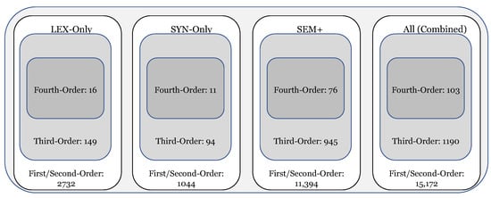
Figure 1.
Break-down of the grammar used in the experiments by construction type.
Thus, the construction in (2) contains three slots, each defined using a syntactic constraint. These constraints are categories learned at the same time that the grammar itself is learned, formulated within an embedding space. An embedding that captures local co-occurrence information is used for formulating syntactic constraints (a continuous bag-of-words fastText model with a window size of 1) while an embedding which instead captures long-distance co-occurrence information is used for formulating semantic constraints (a skip-gram fastText model with a window size of 5). Constraints are then formulated as centroids within that embedding space. Thus, the tokens for the construction in (2) are shown in (2a) through (2d). For the first slot-constraint, the name (determined–permitted) is derived from the lexical items closest to the centroid of the constraint. The proto-type structure of categories is modeled using cosine distance as a measure of how well a particular slot-filler satisfies the constraint. Here, the lexical items “reluctant”, “ready”, “refusal”, and “willingness” appear as fillers sufficiently close to the centroid to satisfy the slot-constraint. The construction itself is a complex verb phrase in which the main verb encodes the agent’s attempts to carry out the event encoded in the infinitive verb. This can be contrasted semantically with the construction in (3), which has the same form but instead encodes the agent’s preparation for carrying out the social action encoded in the infinitive verb. The dialect experiments in this paper rely on type frequency, which means that each construction like (3) is a feature and each unique form like (3a) through (3d) contributes to the frequency of that feature. To describe a larger utterance, these constructions would be clipped together to form longer representations.
| (3) | [ syn: | determined–permitted – syn: to – syn: demonstrate-reiterate ] |
| (3a) | reluctant to speak | |
| (3b) | ready to exercise | |
| (3c) | refusal to recognize | |
| (3d) | willingness to govern |
An important idea in CxG is that structure is learned gradually, starting with item-specific surface forms and moving to increasingly schematic and productive constructions. This is called scaffolded learning because the grammar has access to its own previous analysis for the purpose of building more complex constructions. In computational CxG, this is modeled by learning over iterations with different sets of constraints available. For example, the constructions in (2) and (3) are learned with only access to the syntactic constraints, while the constructions in (4) and (5) have access to lexical and semantic constraints as well. This allows grammars to become more complex while not assuming basic structures or categorizations until they have been learned. In the dialect experiments below, we distinguish between lexical (lex) grammars (which only contain lexical constraints), syntactic (syn) grammars (which contain only syntactic constraints), and sem+ grammars (which contain lexical, syntactic, and semantic constraints).
| (4) | [ lex: | “the” – sem: way – lex: “to” ] |
| (4a) | the chance to | |
| (4b) | the way to | |
| (4c) | the path to | |
| (4d) | the steps to |
Constructions have different levels of abstractness or schematicity. For example, the construction in (4) functions as a modifier, as in the X position in the sentence “Tell me [X] bake yeast bread.” This construction is not purely item-specific because it has multiple types or examples. But, it is less productive than the location-based noun phrase construction in (5) which will have many more types in a corpus of the same size. CxG is a form of lexico-grammar in the sense that there is a continuum between item-specific and schematic constructions, exemplified here by (4) and (5), respectively. The existence of constructions at different levels of abstraction makes it especially important to view the grammar as a network with similar constructions arranged in local nodes within the grammar.
| (5) | [ lex: | “the” – sem: streets ] |
| (5a) | the street | |
| (5b) | the sidewalk | |
| (5c) | the pavement | |
| (5d) | the avenues |
A grammar, or construction, is not simply a set of constructions but rather a network with both taxonomic and similarity relationships between constructions. In computational CxG, this is modeled by using pairwise similarity relationships between constructions at two levels: (i) representational similarity (or how similar the slot-constraints which define the construction are) and (ii) token-based similarity (or how similar are the examples or tokens of two constructions given a test corpus). Matrices of these two pairwise similarity measures are used to cluster constructions into smaller and then larger groups. For example, the phrasal verbs in (6) through (8) are members of a single cluster of phrasal verbs. Each individual construction has a specific meaning: in (6), focusing on the social attributes of a communication event; in (7), focusing on a horizontally situated motion event; in (8), focusing on a motion event interpreted as a social state. These constructions each have a unique meaning but a shared form. The point here is that, at a higher-order of structure, there are a number of phrasal verb constructions which share the same schema. These constructions have sibling relationships with other phrasal verbs and a taxonomic relationship with the more schematic phrasal verb construction. These phrasal verbs are an example of the third-order constructions in the dialect experiments (c.f., ).3
| (6) | [ sem: | screaming–yelling – syn: through ] |
| (6a) | stomping around | |
| (6b) | cackling on | |
| (6c) | shouting out | |
| (6d) | drooling over |
| (7) | [ sem: | rolled–turned – syn: through ] |
| (7a) | rolling out | |
| (7b) | slid around | |
| (7c) | wiped out | |
| (7d) | swept through |
| (8) | [ sem: | sticking–hanging – syn: through ] |
| (8a) | poking around | |
| (8b) | hanging out | |
| (8c) | stick around | |
| (8d) | hanging around |
An even larger structure within the grammar is based on groups of these third-order constructions, structures which we will call fourth-order constructions. A fourth-order construction is much larger because it contains many third-order constructions which themselves contain individual first-order (and second-order) constructions. An example of a fourth-order construction is given with five constructions in (9) through (13) which all belong to same neighborhood of the grammar. The partial noun phrase in (9) points to a particular sub-set of some entity (as in, “parts of the recording”). The partial adpositional phrase in (10) points specifically to the end of some temporal entity (as in, “towards the end of the show”). In contrast, the partial noun phrase in (11) points a particular sub-set of a spatial location (as in, “the edge of the sofa”). A more specific noun phrase in (12) points to a sub-set of a spatial location with a fixed level of granularity (i.e., at the level of a city or state). And, finally, in (13), an adpositional phrase points to a location within a spatial object. Each of these first-order constructions is a member of the same fourth-order construction. This level of abstraction interacts with dialectal variation in that variation and change can take place in reference to either the lower-level or higher-level structures.
| (9) | [ sem: | part – lex: “of” – syn: the ] |
| (9a) | parts of the | |
| (9b) | portion of the | |
| (9c) | class of the | |
| (9d) | division of the |
| (10) | [ syn: | through – sem: which-whereas – lex: “end” – lex: “of” – syn: the ] |
| (10a) | at the end of the | |
| (10b) | before the end of the | |
| (10c) | towards the end of the |
| (11) | [ sem: | which–whereas – sem: way – lex: “of” ] |
| (11a) | the edge of | |
| (11b) | the side of | |
| (11c) | the corner of | |
| (11d) | the stretch of |
| (12) | [ sem: | which–whereas – syn: southside–northside – syn: chicagoland ] |
| (12a) | in north Texas | |
| (12b) | of southern California | |
| (12c) | in downtown Dallas | |
| (12d) | the southside Chicago |
| (13) | [ lex: | “of” – syn: the – syn: courtyard–balcony ] |
| (13a) | of the gorge | |
| (13b) | of the closet | |
| (13c) | of the room | |
| (13d) | of the palace |
The examples in this section have illustrated some of the fundamental properties of CxG and also provide a discussion of some of the features which are used in the dialect classification study. A break-down of the types of constructions found in the grammar is shown in Figure 1. The 15,215 total constructions are first divided into different scaffolds (lex, syn, sem+). As before, lex constructions allow only lexical constraints while sem+ constructions allow lexical and syntactic and semantic constraints. This grammar has a network structure and contains 2132 third-order constructions (e.g., the phrasal verbs discussed above). At an even higher level of structure, there are 97 fourth-order constructions or neighborhoods within the grammar (e.g., the sub-set referencing constructions discussed above). We can thus look at the variation across the entire grammar, across different types of slot-constraints, and across different levels of abstraction when measuring dialect similarity.
To what degree are these grammatical representations adequate across different dialects? This is partly a question of parsing accuracy: do we have more false positives or false negatives in one location (like American English) vs. another (like Indian English)? To evaluate this, we analyze the overall number of constructions found per sample in different countries in Table 2. The basic idea here is that each sample contains the same amount of usage from the same register on the same set of topics; thus, by default, we would expect the same number of constructions to be used. The choice of one construction over another is expected to vary; that is the difference between dialects. But, ideally, the grammar would contain all the constructions used in each dialect so that the total frequency of constructions would be consistent across dialects.
Table 2.
Number of constructions per sample by country (normalized). Higher values indicate more matches per sample, which indicates that the grammar better describes the usage of the dialect.
In practical terms, this is not the case because inner-circle varieties are more likely to be represented in the data used to learn the grammar (), which means that more constructions from inner-circle varieties are likely contained in the grammar. To evaluate the overall parsing quality, we then estimate the total frequency of construction matches per sample per city; since we expect a certain amount of usage to contain a certain number of constructions, higher values mean a better fit with the grammar. Table 2 shows this comparison aggregated to the country level; the values here are standardized so that 1.0, for instance, indicates one standard deviation above the mean. This allows us to compare the different parts of the grammar which have different numbers of matches: first-order and second-order constructions, which are more concrete, and third- and fourth-order constructions, which are more abstract. These results show that the US and Canada have the best fit with the grammar, while India and Pakistan have the worst fit. This evaluation shows that there is a tendency to focus on constructions that better represent some varieties; this implies that city-to-city similarity measures will work better in places like the US. The ranking of countries is largely consistent across levels of abstraction.
Since the grammar is a better fit for certain countries, to what degree is this feature space able to adequately represent variation across dialects on a global scale? We use a classification task to measure the ability to predict the country which each city belongs to in Table 3. First, we estimate the mean type frequency for each construction across samples to provide a single best representation for each city. We then train a linear SVM classifier with different sub-sets of the grammar to predict which country a city belongs to and then evaluate the accuracy of these predictions on held-out cities. The results are divided by the level of abstraction (1st/2nd-, 3rd-, and 4th-order constructions) as well as by the type of representation (lex, syn, sem+). The high prediction accuracy (quantified here by the f-score) indicates that the features are able to adequately distinguish country-level dialects.
Table 3.
F-score for classifying held-out cities by feature type, using type frequencies. A higher f-score indicates that a set of features is able to distinguish between country-level dialects, a validation metric for feature-based similarities.
Thus, Table 3 shows the relative ability of each portion of the grammar to capture country-level variation. We see that less abstract lower-level constructions (first and second order) are most able to capture variation regardless of the type of representation. This is not surprising as grammatical variation is expected to be strongest at these lower levels of abstraction. Next, more abstract features (third order) work well with syn or sem+ representations, but less well with lex representations. And, finally, the most abstract features have the lowest f-scores overall, with sem+ retaining an f-score of 0.82. Again, this follows our expectation: more schematic structures are shared across dialects to a greater degree and thus subject to less variation.
Looking across countries, we see that classification errors are concentrated in outer-circle varieties from places like Indonesia, the Philippines, or Pakistan. Again, these are the varieties least well represented in the frequency evaluation above. Thus, we would expect that city-to-city similarities would be the least precise in these areas. Overall, however, this evaluation shows that even in most outer-circle areas, the prediction accuracy is high, especially with less abstract constructions.
3.3. Measuring Linguistic Similarity
We now have a large number of comparable samples representing 256 cities in English-using countries which have been annotated for constructional features that have themselves been shown capable of distinguishing between country-level dialects. In this context, the annotations are a vector of type frequencies for each construction in the grammar for each sample in the data set. This section discusses the method of calculating pairwise similarities between cities for each of the nine distinct sub-sets of the grammar (i.e., three types of representation at three levels of abstraction).
Pairwise similarity between cities is calculated in three steps: First, we estimate the mean type frequency of each construction across samples for each city and then standardize these estimated frequencies across the entire corpus. Type frequency focuses on the productivity of each construction, and the number of unique forms it takes. This means that we have one expected type frequency per construction per city; values of 1 indicate that a construction is used one standard deviation above the mean across all cities. This standardization ensures that some more frequent constructions do not dominate the comparison. Second, we take the cosine distance between these standardized type frequencies, using as weights the feature loadings from the linear SVM classifier discussed above for country-level dialects. These classification weights focus the cosine distance on those constructions which are subject to variation. Third, because we have no absolute interpretation for pairwise similarities between city-level dialects, we standardize these cosine distances, thus focusing on the relative ranking of similarity values. This produces a ranked list of pairs of cities, with the most similar city-level dialects at the top and the least similar at the bottom.
The accuracy evaluation in Table 3 was focused on validating whether these constructional features are capable, upstream, of distinguishing between dialects in a supervised setting. We follow this with a second accuracy-based validation here in Table 4 which is focused on whether city-to-city similarity measures remain accurate in an unsupervised setting. We first calculate, for each city, the distance with all other cities. Secondly, we compare the distances of (i) within-country cities and (ii) out-of-country cities. An accurate prediction is when each city is closest to other cities within the same country. This measure of accuracy is shown in Table 3 across levels of abstraction (first/second-, third-, and fourth-order constructions) and across levels of representation (lex, syn, and sem+, which contains all three types of representation).
Table 4.
Accuracy evaluation of weighted similarity scores by feature type with type frequencies. High accuracy means that cities within the same country are most similar to other cities from the same country, rather than external cities.
Our main concern is that these pairwise similarity measures are sufficiently accurate that the rankings can be taken as representing actual similarity between dialects within some portion of the grammar. As before, less abstract features (first/second- and third-order constructions) have higher accuracy because they are subject to more variation. Note that, by using type frequency as a means of comparison, we are looking at the relative productivity of each construction rather than differences in specific forms. Thus, the same construction could be equally productive in two dialects, while producing different forms in each. The lowest accuracy is found in the most abstract features (third-order constructions); to some degree, we expect that the most schematic constructions are subject to less variation. Within these features, the lowest performing areas are outer-circle varieties from Indonesia and Malaysia. It should be noted that predicting that a city is closest to another city in a neighboring country is not necessarily incorrect (i.e., in border areas); for our purposes, we would expect within-country similarity to be higher in most but not all cases.
A final approach to evaluating the robustness of this operationalization of construction grammar is to measure the degree to which we would reach the same measures of city-level dialect similarity given random permutations of the grammar. The similarity measure outputs a rank of over 30 k cities, from most to least similar. In this evaluation, we randomly remove a certain percentage of the constructions and then recalculate this similarity ranking. This is shown in Figure 2, using the Pearson correlation to measure how similar two rankings are high values indicate that a particular grammar is very similar to the full grammar in terms of how it ranks cities. Thus, high correlations show that the feature space is robust to random permutations. The x axis shows increasing percentages of permutations. For instance, at 0.2, we randomly remove 20% of the constructions and recalculate the distances between cities. Each level is computed 10-times and then averaged (a 10-fold cross-validation at each step).
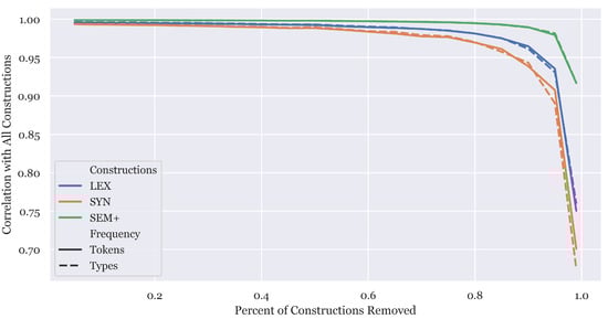
Figure 2.
Robustness of city-level similarity ranks across random permutations in the grammar.
The figure divides the grammar by the type of representation (lex, syn, sem+) and also by token frequency vs. type frequency for measuring the construction usage. This figure shows that up to 80% of the constructions can be removed before significant impacts are seen on the city-level similarity ranks. This indicates that the distance matrix used in these experiments is highly robust to random variations in the grammar induction component used to form the feature space. Thus, we should have high confidence in this operationalization of the grammar. This converges with the accuracy-based evaluations which also show that this feature space is able to identify the political boundaries which separate cities.
3.4. Social and Geographic Variables
We have now discussed comparable corpora across 256 cities which are annotated for constructional features in a way that supports accurate pairwise similarity measures between cities. These grammatical similarity measures tell us about dialectal variation in different portions of the grammar, about the patterns of diffusion for syntactic variants. The research question here is about the factors which cause or at least influence these similarity patterns: why are some dialects of English more similar than others? In this paper, we experiment with three factors: (1) the geographic distance between cities, (2) the amount of population contact between cities as measured by air travel, and (3) the language contact experienced within each city as measured by the linguistic landscape of each city. This section describes each of these three measures. This builds on previous work combining dialectology with social and environmental variables (; ).
The simplest of these three measures is geographic distance; here, we use the geodesic distance measured in kilometers. This approach accounts for the shape of the Earth but not for intervening features like mountains or oceans. We exclude pairs of cities which are closer than 250 km from one another; for such a close comparison, for instance, data from air travel is likely to greatly underestimate the amount of contact between two populations.
The second measure is the amount of population contact, for which we use as a proxy the number of airline passengers traveling from one city to another (). This flight-based variable can be consistently calculated for all the cities in this study and provides a generic measure of the amount of travel between cities which is itself a proxy for the amount of mutual exposure between the two local populations. Especially for long-distance pairs, air travel is often the only practical method for such travel. To make the travel measure symmetric, we combine trips in both directions (e.g., Chicago to Christchurch and Christchurch to Chicago). To illustrate why we include both geographic distance and the amount of air travel as factors, there is a negative Pearson correlation of −0.147 between the two factors. This means that there is not a close relationship between the two, so that each retains unique information about the relationship between cities.
The third measure captures differences in language contact based on the linguistic landscape in a city, motivated by work on the types of language contact involved in variation (). We use tweet-based data for this, focusing on the digital landscape because we are observing digital language use on the same platform. We take all tweets within 200 km of a city which are closer to that city than to any other. Then, using the geographic GeoLID model (), we find the relative frequency of up to 800 languages. The distance between two cities is then the cosine distance between this measure of the relative usage of languages. The more similar two cities are, the more they are experiencing the same types of language contact.
Examples of three pairs of cities are shown in Table 5, with the distance between the linguistic landscape together with the break-down of most-used languages. The most different landscapes are between Glasgow (UK) and Jakarta (ID), at 0.819. English is the majority language in Glasgow (90%) but only a minority language in Jakarta (11.8%). Beyond this, Jakarta has a high use of Austronesian languages while Glasgow has very little. The next pair is Auckland (NZ) and Montreal (CA). In both bases, English is the most common, but in Montreal it constitutes only 54.7%, with French contributing 35%. Auckland is mostly characterized, however, by relatively small amounts of usage from languages like Spanish or Portuguese or Indonesian. And, finally, there is no distance at all between Oklahoma City (US) and Regina (CA), both with a high majority of English usage. These examples show three positions on the continuum between similar or different linguistic landscapes using this measure. Populations with different linguistic landscapes have, as a result, experienced different types of language contact. For instance, English in Jakarta has had a high amount of contact with Indonesian while, in Montreal, English has had a high amount of contact with French.
Table 5.
Examples of linguistic landscape measures, calculated as the relative usage of languages in tweets within 200 km of each city. High values indicate a different mix of languages in each city. This is used as a proxy for differences in the language contact experienced by different cities.
These three external features, the geographic distance, population contact, and language contact, are used as possible factors that could explain pairwise grammatical similarities between English-using cities around the world. We might expect, for instance, that closer cities are more similar linguistically (with certain thresholds to control for settler nations like New Zealand that are far from Europe). And, we might expect that dialects where English is mixing with French, for instance, would be more similar to other French-influenced dialects. The following section undertakes this analysis.
4. Results
This section uses a regression analysis and a clustering analysis to determine whether external factors like language contact and population contact influence the network of dialect similarities. Our first question is whether the different sub-sets of the grammar agree in their ranking of cities by similarity. If different feature sets largely agree, then analyzing each individually is redundant. Put another way, if the grammar is structured as a network and if processes of diffusion are influenced by this network structure, it follows that the network of dialect similarities will depend on the portion of the grammar being observed. For instance, previous work has shown that, in dialects of Dutch, there is the least correspondence between lexical and syntactic variables in terms of the ranks of dialect similarity (). Here, we examine correlations between types of representations in Figure 3, using the Pearson correlation between ranks of cities derived from each of the nine sub-sets of the grammar (by level of abstraction and type of representation).
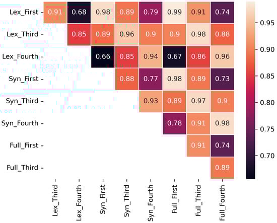
Figure 3.
Pearson correlations between ranks of pairwise similarity between cities for different sub-sets of the grammar.
Similarity ranks are significantly influenced by the part of the grammar being observed, with some correlations as low of 0.68 (across levels of abstraction with lex representations) or 0.66 (across type of representation from lex to syn). This means that the network structure of the grammar has influenced diffusion. Thus, we undertake the analysis across each of the portions of the grammar separately: the nine specific sub-sets in addition to a concatenation of all representation types (called all). In other words, this lower level of correlation means that two local dialects have experienced the same diffusion processes in some strata of the construction but not in others.
We use multivariate linear regression analysis (MLRA) to test our hypothesis that these dialect similarity networks can be predicted by (i) language contact and (ii) population contact between local areas. The MLRA method allows us to test a large number of outcome variables with a single set of predictor variables. The key assumptions of the MLRA method are that there is a linear relationship between the outcome and predictor variables and that the variables follow a normal distribution. Therefore, we conducted exploratory data analysis on the predictor and outcome variables. The outcome variables involved in our MLRA analysis include the twelve sub-sets of the grammar (c.f. Figure 1). The predictor variables included three external variables and eight derived variables as discussed in Section 3.4. The external outcome variables included the following:
- : the frequency of airline travel between two cities;
- : the raw geographic distance between two cities;
- : the difference in the linguistic landscape between two cities.
The predictor variables in our MLRA analysis include whether the origin and destination country () or region () are the same or different; thus, two cities in the US would have the status Same. In addition to these predictor variables, we also use geographic predictor variables, including the origin and destination city ( and ), country ( and ), and region ( and ). These variables allow us to control for specific local dialects with idiosyncratic patterns. The final dataset includes 29,253 pairwise observations (because cities too close together were excluded from this analysis). It is important to note that the three external predictor variables are not normally distributed (i.e., some places like cities in New Zealand are extremely far from most other cities).
As shown in Figure 4, the first/second-order and third-order outcome variables are normally distributed with a slight negative skew, while the fourth-order outcome variables have a bimodal distribution with peaks towards the start and the end of the distribution. In order to address these non-normal distributions, we apply log-transformations on the relevant variables.
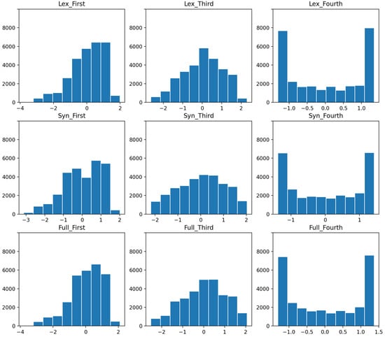
Figure 4.
Distribution of type frequencies per sample by sub-set of the grammar.
Our model selection criteria is informed by the model performance metrics from the analysis of variance (ANOVA) test. The full suite of predictors used in our MLRA analysis are listed below from (14a) to (14e). We start with larger models that encompass all predictor variables and then move toward smaller models focused on specific factors.
| (14a) | |
| (14b) | |
| (14c) | |
| (14d) | |
| (14e) |
Our maximal model (14a) includes all three external predictor variables (, , and ) and two derived variables ( and ), while our minimal model (14e) includes only the interaction between the two log-transformed external predictor variables ( and ). We do not include the geographically derived predictor variables (i.e., ) as these variables are more suited as random effects due to the large number of categories. The results of the MLRA analysis are shown in Table 6.
Table 6.
Model performance statistics for the MLRA model (14a) to (14e) from the multivariate ANOVA including the degrees of freedom (Df), Pillai’s trace (Pillai), variation between means/variation within the samples (F), and the p-value of the F-statistic (Pr(>F)).
While all candidate models provided statistically significant results as standalone models, only three candidate models (14b, 14d, and 14e) yielded statistical significance according the results of the multivariate ANOVA with reference to Table 6. (14d) had the best performance compared to (14b) and (14d) based on the F-statistic. We provided the variable-level model performance statistics for (14d) in Table 7. The model performance statistics suggest that all three predictors (, , and ) are statistically significant, and that there is explanatory value in the interaction between the two external predictor variables ( and ).
Table 7.
Model performance statistics for the MLRA model 14d from the multivariate ANOVA including the degrees of freedom (Df), Pillai’s trace (Pillai), variation between means/variation within the samples (F), and the p-value of the F-statistic (Pr(>F)).
This result is unsurprising as the MLRA assumes a linear relationship between variables; which may explain why the log-transformed predictor variables outperformed the non-normalized predictor variables. The low explanatory value of may stem from the variable itself; although travel with up to three connecting cities is included, most travel is between a relatively small portion of the cities; passenger numbers do not control for the size of a city’s population. In other words, city-level air travel may not adequately operationalize population contact. Additionally, we cannot log-transform missing data and many pairs of cities have no direct travel. One statistical test we use is the Pillai score, or Pillai’s trace, which is a measure of linear dependence between two categories. A small Pillai score suggests there is insufficient evidence to reject the null hypothesis. What is surprising is that all three candidates models (14b, 14d, 14e) provided a small value which suggests there is insufficient evidence to reject the null hypothesis. Therefore, we also included the origin region () as a fixed effect to determine this pattern at the city-level in addition to the first suite of MLRA models. We only included the external predictor variables with the greatest explanatory power in our models ( and ).
| (15a) | |
| (15b) | |
| (15c) |
Once again, all candidate models provided statistically significant results as standalone models. However, only 15b was considered statistically significant based on the model performance statistics of the multivariate ANOVA. We provided the variable-level model performance statistics for 15b in Table 8.
Table 8.
Model performance statistics for the MLRA model 15b from the Multivariate ANOVA including the degrees of freedom (Df), Pillai’s trace (Pillai), variation between means/variation within the samples (F), and the p-value of the F-statistic (Pr(>F)).
The external predictor variable, , no longer held any explanatory value when we included the predictor variable . The high value associated with in 15b suggests that we fail to reject the null hypothesis. Our analysis thus suggests that language contact and population contact between local areas are predictors of grammatical similarity; however, geographic variables about region or country membership are more important than those two variables. While these factors are significant, there is also a great deal of variation in dialect similarity which is not explained by them.4
Clustering Analysis
This section presents an additional cluster-based analysis. The regression-based analysis takes a linear view of the problem: the travel between Chicago and Christchurch, for example, is viewed as completely independent as travel between Indianapolis and Dunedin. We might expect diffusion to take a hub-and-spoke model; however, which would mean that local structures in the network would be important. We approximate local structures using HDBSCAN (hierarchical density-based spatial clustering of applications with noise), a bottom–up clustering algorithm which allows clusters of different sizes and densities. This is an important property given that the geographic distribution of the dialect areas is very heterogeneous (e.g., dense in some parts of the US while very sparse in parts of Australia).
We cluster cities based on each of the variables, both linguistic (i.e., a type of construction) and social (i.e., language contact). This allows us to compare clusters based on different types of information. The distribution of clusters based on geographic distance results in either country-level or sub-country groupings depending on the size of the country. These form the ground-truth, the spatial clusters of cities without any linguistic information. We then do clustering based on linguistic features; this is shown with the third-order sem+ grammar in Table 9. This clustering has no access to geographic information, based entirely on linguistic distances between cities. And yet, it closely matches the geographic clusters; the adjusted mutual information score between geographic clusters and these grammar-based clusters is a relatively high 0.66. All clusters are contiguous spatially and only three clusters cross national borders: one that joins Pakistan and Western India, one that joins Ontario with the upper Midwest, and one that joins Seattle and Vancouver. This shows that, taking into account larger network effects, the grammatical distances largely correspond to physical distances.
Table 9.
Overlap as measured by Adjusted Mutual Information between clusters formed with external information (language contact and geographic distance) those formed with sub-sets of the grammar. Higher measures mean more overlap.
Cluster assignments within North America are shown in Table 10, showing how grammar-based clusters (without access to geography) align with geographic patterns. The first column shows US-only clusters, the second shows CA-only clusters, and the third shows mixed clusters. The first mixed cluster contains two near-by cities, Seattle and Vancouver. The second crosses the upper Midwest and Ontario (with some outliers, like Nashville and Louisville). Other clusters conform to geographic pairings: for instance, there is a Texas cluster (#28) and a mid-Atlantic cluster (#21) and a California cluster (#37). Thus, grammatical information alone provides meaningful similarities, something we have already seen in previous evaluations.
Table 10.
Grammar-based clusters (third-order Sem+ constructions) within North America. Cluster numbers are arbitrary.
The main question here is the degree to which grammatical distances overlap with social factors like geographic distance, population contact, and language contact. Unfortunately, clusters derived from population contact are ill-formed because many pairs of cities have no travel information (our proxy for population contact), posing a challenge for an approach based on a symmetrical distance metric. This is shown in Table 9 with the language contact and geographic distance clusters, using adjusted mutual Information. Higher values indicates a higher overlap with these factors, meaning they are more important. We see, first, that language contact is usually more important than geographic distance and, second, that both create meaningful overlaps. This indicates that, when taking a larger network structure into account, these factors are important for the organization of linguistic distances. This, in turn, means that these external factors can be seen as forces driving dialectal variation.
5. Discussion and Conclusions
This paper has used comparable samples of geo-referenced tweets to construct highly-accurate construction-based similarity measures between 256 city-level dialects of English. These pairwise similarities reflect synchronic network relationships between local dialects, a network with approximately 30,000 nodes (with very close cities not compared). Given this representation of grammatical variation, we ask whether the properties of the network are driven by external variables like the amount of language contact or population contact or geographic distance.
The results show that all of these variables create regression models with significant explanatory value. The best models, however, rely on (i) language contact, (ii) geographic distance, and (iii) region information. Thus, population contact as operationalized by air travel is not among the best predictors of dialect similarity. We recognize that these measures are only an abstraction of real-world geographic processes. Overall, this study provides a large-scale data-driven approach to evaluating which social factors are most important for diffusion. The diachronic processes of diffusion are responsible for the synchronic similarity networks we are now observing, so that this is an approach to understanding how constructions are spread from one population to another.
The regression-based analysis in this paper shows that these explanatory values have significant impacts on dialect similarity. This finding is not the end of the story, however. This is because the regression models flatten out the dialect similarity network into sets of pairs. This is important for establishing that the similarity between local dialects is influenced by these external factors, but a network-based approach would provide a better view of the processes of diffusion. For example, large amounts of travel between Chicago and Jakarta would have no influence on cities close to Chicago or Jakarta in this model.
Beyond finding predictor variables that help to explain dialect similarity, a fully network-based approach would support an understanding of the flow of constructions as they spread from one dialect to another. The results in this current study establish that construction-based similarity networks are accurate and that they are especially influenced by geographic distance and language contact and region membership. This further validates the similarity measures themselves and paves the way for a more detailed network-based analysis of the diffusion of constructions.
Finally, we conclude by considering two potentially limiting assumptions in this work: that social media data captures a vernacular register and that the aggregate properties of a population (like the potential for language contact) can be disaggregated into individual factors. Here, we consider each of these assumptions in turn.
In the first case, social media data, as a source of evidence about language, is neither speech nor writing. On the one hand, previous work has shown that lexical dialectology can be replicated using social media data (), at least for the UK. This would suggest that social media data, although written, provides an approximation for speech. On the other hand, we would argue that, because of the presence of register variation, there is no one ground-truth modality for observing dialectal variation. Thus, if dialect and register co-vary, the main criteria for studying dialects is that the register be held constant. If we were using social media to observe the UK but a switchboard corpus to observe New Zealand and a radio corpus to observe Singapore, then register would interfere with our observations. But, if we hold the register constant, then any register would in theory be sufficient for evaluating the factors which cause grammatical variation.
In the second case, we have estimated both grammatical similarity and external factors like exposure to language contact in the aggregate. And yet, every individual in a city has their own linguistic experiences. You might argue, for example, that length of stay, social networks, and other individualized behaviors would need to be considered instead of aggregate travel patterns. In the same way, you might argue that language contact as a factor in dialect differentiation is only viable at the individual level because it is part of the linguistic experience of individuals. We can argue against this position in two ways: First, from an empirical perspective, our analysis here shows that language contact in the aggregate is a significant predictor of dialect similarity. If aggregate properties were meaningless, then predictors based on aggregate properties would fail; but they do not. Second, from a theoretical perspective, we have to remember that realistic contact networks span many more speakers than traditional studies can capture (; ). If we were to include all indirect contact, then an aggregate approach to language contact might well fare better as a predictor: any given individual, for instance, does not know the contact experienced by each and every of their own interlocutors. In this case, it is an empirical question whether disaggregated contact (as in this study) or individualized contact (as a potential alternate approach) is a better predictor. But, regardless, the point of this paper has been to construct a natural experiment capable of determining which factors best describe the syntactic relationships between dialects.
Author Contributions
Conceptualization, J.D. and S.W.; methodology, J.D. and S.W.; software, J.D.; validation, J.D. and S.W.; resources, J.D.; data curation, J.D.; writing—original draft preparation, J.D. and S.W.; writing—review and editing, J.D. and S.W.; visualization, J.D. and S.W. All authors have read and agreed to the published version of the manuscript.
Funding
This research received no external funding.
Data Availability Statement
The data and supplementary material for this paper is available at https://doi.org/10.17605/OSF.IO/GD2KQ.
Conflicts of Interest
The authors declare no conflicts of interest.
Abbreviations
The following abbreviations are used in this manuscript:
| ZA | South Africa |
| KE | Kenya |
| NG | Nigeria |
| CA | Canada |
| US | United States |
| IN | India |
| PK | Pakistan |
| ID | Indonesia |
| MY | Malaysia |
| PH | Philippines |
| UK | United Kingdom |
| AU | Australia |
| NZ | New Zealand |
| ENG | English |
| SCO | Scots |
| IND | Indonesian |
| JAV | Javanese |
| SUN | Sundanese |
| BJN | Banjarese |
| FRA | French |
| SPA | Spanish |
| POR | Portuguese |
| ARA | Arabic |
| TGL | Tagalog |
| KOR | Korean |
| CGLU | Corpus of Global Language Use |
| CxG | Construction grammar |
| LEX | Constructions with lexical slot-constraints |
| SYN | Constructions with syntactic slot-constraints |
| SEM | Constructions with semantic slot-constraints |
| SEM+ | Constructions with lexical, syntactic, and semantic slot-constraints |
| SVM | Support vector machine |
| MLRA | Multivariate linear regression analysis |
| ANOVA | Analysis of variance |
Appendix A. City Locations by Country
Table A1.
Locations of cities by country, inner-circle. Some larger cities are divided into sub-regions and distinguished using the airport code for the nearest airport.
Table A1.
Locations of cities by country, inner-circle. Some larger cities are divided into sub-regions and distinguished using the airport code for the nearest airport.
| Australia (AU) | |||
| Adelaide | Brisbane | Cairns | Canberra |
| Darwin | Hobart | Launceston | Melbourne (meb) |
| Melbourne (mel) | Newcastle | Perth | Sunshine Coast |
| Sydney | Toowoomba | Townsville | |
| Canada (CA) | |||
| Abbotsford | Calgary | Edmonton | Halifax |
| Hamilton | Kelowna | Kingston | Kitchener |
| London | Montreal (yhu) | Montreal (yul) | Ottawa |
| Quebec | Regina | Saint John | Saskatoon |
| Sudbury | Thunder Bay | Toronto (ytz) | Toronto (yyz) |
| Vancouver (cxh) | Vancouver (yvr) | Windsor | Winnipeg |
| New Zealand (NZ) | |||
| Auckland | Christchurch | Dunedin | Hamilton |
| Tauranga | Wellington | ||
| United Kingdom (UK) | |||
| Aberdeen | Belfast | Birmingham | Blackpool |
| Bournemouth | Bristol | Cardiff | Dundee |
| Edinburgh | Exeter | Glasgow | Gloucester |
| Leeds | Leicestershire | Liverpool | London (lcy) |
| London (lgw) | London (lhr) | London (ltn) | London (stn) |
| Manchester | Newcastle | Plymouth | Southampton |
| Southend | |||
| United States (US) | |||
| Akron/Canton | Albuquerque | Anchorage | Atlanta |
| Austin | Bakersfield | Baltimore | Baton Rouge |
| Birmingham | Boston | Buffalo | Burbank |
| Charlotte | Chicago | Cincinnati | Cleveland |
| Colorado Springs | Corpus Christi | Dallas (dal) | Dallas (dfw) |
| Denver | Fort Wayne | Fresno | Gainesville |
| Geensboro | Honolulu | Houston | Indianapolis |
| Kansas City | Las Vegas | Lexington | Lincoln |
| Long Beach | Louisville | Lubbock | Madison |
| Memphis | Mesa | Miami | Milwaukee |
| Minneapolis | Modesto | Nashville | New Orleans |
| New York | Newark | Norfolk | Oakland |
| Oklahoma City | Omaha | Ontario | Orlando |
| Philadelphia | Phoenix | Pittsburgh | Raleigh/Durham |
| Rochester | Sacramento | Saint Louis | Saint Petersburg |
| San Antonio | San Diego | San Francisco | San Jose |
| Santa Ana | Seattle | Stockton | Tampa |
| Toledo | Tulsa | Washington | Wichita |
Table A2.
Locations of cities by country, outer-circle. Some larger cities are divided into sub-regions and distinguished using the airport code for the nearest airport.
Table A2.
Locations of cities by country, outer-circle. Some larger cities are divided into sub-regions and distinguished using the airport code for the nearest airport.
| Indonesia (ID) | |||
| Bandar Lampung | Bandung | Jakarta | Medan |
| Semarang | Tanjung Pinang | ||
| India (IN) | |||
| Agra | Ahmedabad | Allahabad | Amritsar |
| Aurangabad | Bangalore | Bhavnagar | Bhopal |
| Bhubaneswar | Chandigarh | Chennai | Coimbatore |
| Dehra Dun | Delhi | Gaya | Gorakhpur |
| Hubli | Hyderabad | Indore | Jabalpur |
| Jaipur | Jammu | Jamnagar | Jodhpur |
| Kanpur | Kochi | Kolhapur | Kolkata |
| Kozhikode | Lucknow | Ludhiana | Madurai |
| Mangalore | Mumbai | Nagpur | Pantnagar |
| Patna | Pune | Raipur | Rajkot |
| Ranchi | Salem | Thiruvananthapuram | Tuticorin |
| Udaipur | Vadodara | Varanasi | Vijayawada |
| Vishakhapatnam | |||
| Kenya (KE) | |||
| Arusha | Eldoret | Kilimanjaro | Kisumu |
| Mombasa | Musoma | Nairobi (nbo) | Nairobi (wil) |
| Samburu | |||
| Malaysia (MY) | |||
| Ipoh | Johor Bharu | Kota Kinabalu | Kuala Lumpur (kul) |
| Kuala Lumpur (szb) | Kuantan | Penang | Singapore |
| Nigeria (NG) | |||
| Abuja | Akure | Benin City | Enugu |
| Jos | Kaduna | Lagos | Owerri |
| Port Harcourt | Warri | ||
| Philippines (PH) | |||
| Bacolod | Cagayan De Oro | Cebu | Davao |
| Dumaguete | Manila | Naga | Ozamis City |
| Pakistan (PK) | |||
| Bahawalpur | Dera Ismail Khan | Faisalabad | Hyderabad |
| Islamabad | Karachi | Lahore | Multan |
| Nawabshah | Quetta | Rahim Yar Khan | Sialkot |
| Sukkur | |||
| South Africa (ZA) | |||
| Bloemfontein | Cape Town | Durban | East London |
| George | Johannesburg | Nelspruit | Pietermaritzburg |
| Polokwane | Port Elizabeth | Richards Bay | |
Appendix B. Keywords
Table A3.
Keywords used to create lexically balanced samples. Words are listed in order of frequency.
Table A3.
Keywords used to create lexically balanced samples. Words are listed in order of frequency.
| know | time | people | day | love | new |
| see | think | why | here | want | go |
| really | need | today | make | still | because |
| first | very | best | after | than | never |
| got | much | back | please | going | great |
| right | then | life | thank | well | way |
| always | year | over | world | most | take |
| man | say | last | let | into | work |
| where | other | look | many | said | off |
| same | years | which | game | video | better |
| come | something | happy | thanks | via | yes |
| down | hope | god | stop | give | ever |
| feel | everyone | big | team | help | live |
| getting | while | use | keep | things | another |
| long | week | sure | days | watch | real |
| looking | shit | against | actually | doing | money |
| free | show | since | home | lot | nothing |
| bad | find | already | read | through | part |
| tell | without | won | such | start | little |
| play | thought | everything | morning | old | support |
| person | call | done | check | mean | news |
| put | both | wait | women | end | believe |
| used | top | around | night | looks | family |
| name | country | yeah | anyone | between | gonna |
| trying | says | hard | guys | maybe | friends |
| point | beautiful | remember | win | full | sorry |
| follow | government | high | during | amazing | yet |
| making | school | under | anything | coming | state |
| post | away | guy | change | try | house |
| open | might | season | whole | makes | left |
| song | media | saying | few | using | president |
| different | enough | black | called | talk | trump |
| place | talking | friend | care | power | once |
| wrong | city | working | nice | ready | times |
| business | understand | set | music | join | buy |
| vote | hate | heart | future | girl | mind |
| wish | face | seen | tomorrow | found | needs |
| watching | party | though | playing | least | problem |
| stay | covid | project | head | kind | white |
| group | health | until | food | story | cause |
| literally | soon | men | congratulations | job | ask |
| police | human | saw | waiting | far |
Notes
| 1 | https://www.earthLings.io, accessed on 19 July 2025. |
| 2 | https://github.com/jonathandunn/c2xg/tree/v2.0, accessed on 19 July 2025. |
| 3 | Available at https://www.jdunn.name/cxg, accessed on 19 July 2025. |
| 4 | Not included in this results section are additional tests where we found that substituting the log-transformation normalization method with the z-score standardization did not improve model performance; nor did we find improvements to model performance by excluding city pairs with no airline travel (pop_contact). |
References
- Anthonissen, L. (2020). Cognition in construction grammar: Connecting individual and community grammars. Cognitive Linguistics, 31(2), 309–337. [Google Scholar] [CrossRef]
- Barbaresi, A. (2018). Computationally efficient discrimination between language varieties with large feature vectors and regularized classifiers. In Proceedings of the fifth workshop on NLP for similar languages, varieties and dialects (pp. 164–171). Association for Computational Linguistics. [Google Scholar]
- Beckner, C., Ellis, N., Blythe, R., Holland, J., Bybee, J., Ke, J., Christiansen, M., Larsen-Freeman, D., Croft, W., & Schoenemann, T. (2009). Language is a complex adaptive system: Position paper. Language Learning, 59, 1–26. [Google Scholar] [CrossRef]
- Belinkov, Y., & Glass, J. (2016). A character-level convolutional neural network for distinguishing similar languages and dialects. In Proceedings of the third workshop on NLP for similar languages, varieties and dialects (pp. 145–152). Association for Computational Linguistics. [Google Scholar]
- Chakravarthi, B. R., Mihaela, G., Tudor Ionescu, R., Jauhiainen, H., Jauhiainen, T., Lindén, K., Ljubešić, N., Partanen, N., Priyadharshini, R., Purschke, C., Rajagopal, E., Scherrer, Y., & Zampieri, M. (2021). Findings of the VarDial evaluation campaign 2021. In Proceedings of the eighth workshop on NLP for similar languages, varieties and dialects, Kiyv, Ukraine, April 20. Association for Computational Linguistics. [Google Scholar]
- Cook, P., & Brinton, J. (2017). Building and evaluating web corpora representing national varieties of English. Language Resources and Evaluation, 51(3), 643–662. [Google Scholar] [CrossRef]
- Croft, W. (2020). English as a lingua franca in the context of a sociolinguistic typology of contact languages. In A. Mauranen, & S. Vetchinnikova (Eds.), Language change: The impact of English as a lingua franca (pp. 44–74). Cambridge University Press. [Google Scholar]
- Davies, M., & Fuchs, R. (2015). Expanding horizons in the study of world Englishes with the 1.9 billion word global web-based English corpus (GloWbE). English World-Wide, 36(1), 1–28. [Google Scholar] [CrossRef]
- Dąbrowska, E. (2021). How writing changes languages. In Language change: The impact of English as a lingua franca (pp. 75–94). Cambridge University Press. [Google Scholar] [CrossRef]
- Diessel, H. (2023). The constructicon: Taxonomies and networks. Elements in construction grammar. Cambridge University Press. [Google Scholar] [CrossRef]
- Donoso, G., Sánchez, D., & Sanchez, D. (2017). Dialectometric analysis of language variation in Twitter. In Proceedings of the fourth workshop on NLP for similar languages, varieties and dialects (VarDial), Valencia, Spain, April 3 (Volume 4, pp. 16–25). Association for Computational Linguistics. [Google Scholar] [CrossRef]
- Doumen, J., Beuls, K., & Van Eecke, P. (2023). Modelling language acquisition through syntactico-semantic pattern finding. In A. Vlachos, & I. Augenstein (Eds.), Findings of the association for computational linguistics: EACL 2023, Dubrovnik, Croatia, May 2–6 (pp. 1347–1357). Association for Computational Linguistics. [Google Scholar] [CrossRef]
- Doumen, J., Beuls, K., & Van Eecke, P. (2024). Modelling constructivist language acquisition through syntactico-semantic pattern finding. Royal Society Open Science, 11, 231998. [Google Scholar] [CrossRef]
- Dunn, J. (2018). Finding variants for construction-based dialectometry: A corpus-based approach to regional cxgs. Cognitive Linguistics, 29(2), 275–311. [Google Scholar] [CrossRef]
- Dunn, J. (2019a). Global syntactic variation in seven languages: Toward a computational dialectology. Frontiers in Artificial Intelligence, 2, 15. [Google Scholar] [CrossRef]
- Dunn, J. (2019b). Modeling global syntactic variation in English using dialect classification. In Proceedings of the sixth workshop on NLP for similar languages, varieties and dialects (pp. 42–53). Association for Computational Linguistics. [Google Scholar]
- Dunn, J. (2020). Mapping languages: The corpus of global language use. Language Resources and Evaluation, 54, 999–1018. [Google Scholar] [CrossRef]
- Dunn, J. (2023). Syntactic variation across the grammar: Modelling a complex adaptive system. Frontiers in Complex Systems, 1, 1273741. [Google Scholar] [CrossRef]
- Dunn, J. (2024a). Computational construction grammar: A usage-based approach. Cambridge University Press. [Google Scholar] [CrossRef]
- Dunn, J. (2024b). Validating and exploring large geographic corpora. In N. Calzolari, M.-Y. Kan, V. Hoste, A. Lenci, S. Sakti, & N. Xue (Eds.), Proceedings of the 2024 joint international conference on computational linguistics, language resources and evaluation (LREC-COLING 2024), Torino, Italia, May 20–25 (pp. 17348–17358). ELRA and ICCL. [Google Scholar]
- Dunn, J., Adams, B., & Madabushi, H. T. (2024). Pre-trained language models represent some geographic populations better than others. In N. Calzolari, M.-Y. Kan, V. Hoste, A. Lenci, S. Sakti, & N. Xue (Eds.), Proceedings of the 2024 joint international conference on computational linguistics, language resources and evaluation (LREC-COLING 2024), Torino, Italia, May 20–25 (pp. 12966–12976). ELRA and ICCL. [Google Scholar]
- Dunn, J., & Edwards-Brown, L. (2024). Geographically-informed language identification. In N. Calzolari, M.-Y. Kan, V. Hoste, A. Lenci, S. Sakti, & N. Xue (Eds.), Proceedings of the 2024 joint international conference on computational linguistics, language resources and evaluation (LREC-COLING 2024), Torino, Italia, May 20–25 (pp. 7672–7682). ELRA and ICCL. [Google Scholar]
- Dunn, J., & Madabushi, H. T. (2021). Learned construction grammars converge across registers given increased exposure. In Conference on computational natural language learning. Association for Computational Linguistics. [Google Scholar] [CrossRef]
- Dunn, J., & Nijhof, W. (2022). Language identification for austronesian languages. In Proceedings of the 13th international conference on language resources and evaluation (pp. 6530–6539). European Language Resources Association. [Google Scholar]
- Dunn, J., & Wong, S. (2022). Stability of syntactic dialect classification over space and time. In Proceedings of the 29th international conference on computational linguistics, Gyeongju, Republic of Korea, October 12–17 (pp. 26–36). International Committee on Computational Linguistics. [Google Scholar]
- Eisenstein, J., O’Connor, B., Smith, N., & Xing, E. (2014). Diffusion of lexical change in social media. PLoS ONE, 10, 1371. [Google Scholar] [CrossRef] [PubMed]
- Fagyal, Z., Swarup, S., Escobar, A. M., Gasser, L., & Lakkaraju, K. (2010). Centers and peripheries: Network roles in language change. Lingua, 120(8), 2061–2079. [Google Scholar] [CrossRef]
- Fonteyn, L., & Nini, A. (2020). Individuality in syntactic variation: An investigation of the seventeenth-century gerund alternation. Cognitive Linguistics, 31(2), 279–308. [Google Scholar] [CrossRef]
- Goebl, H. (2006). Recent advances in Salzburg dialectometry. Literary and Linguistic Computing, 21(4), 411–435. [Google Scholar] [CrossRef]
- Gonçalves, B., Loureiro-Porto, L., Ramasco, J. J., & Sánchez, D. (2018). Mapping the Americanization of English in space and time. PLoS ONE, 13(5), e0197741. [Google Scholar] [CrossRef]
- Gonçalves, B., & Sánchez, D. (2014). Crowdsourcing dialect characterization through twitter. PLoS ONE, 9(11), e112074. [Google Scholar] [CrossRef]
- Gooskens, C. (2005). Travel time as a predictor of linguistic distance. Dialectologia et Geolinguistica, 2005(13), 38–62. [Google Scholar] [CrossRef]
- Grafmiller, J., & Szmrecsanyi, B. (2018). Mapping out particle placement in Englishes around the world: A study in comparative sociolinguistic analysis. Language Variation and Change, 30(3), 385–412. [Google Scholar] [CrossRef]
- Grieve, J. (2011). A regional analysis of contraction rate in written Standard American English. International Journal of Corpus Linguistics, 16(4), 514–546. [Google Scholar] [CrossRef]
- Grieve, J. (2016). Regional variation in written American English. Cambridge University Press. [Google Scholar]
- Grieve, J., Montgomery, C., Nini, A., Murakami, A., & Guo, D. (2019). Mapping lexical dialect variation in British English using Twitter. Frontiers in Artificial Intelligence, 2, 11. [Google Scholar] [CrossRef]
- Heeringa, W., Kleiweg, P., Gooskens, C., & Nerbonne, J. (2006). Evaluation of string distance algorithms for dialectology. In Workshop of the Workshop on Linguistic Distances (pp. 51–62). Association for Computational Linguistics. [Google Scholar]
- Hoffmann, T., & Trousdale, G. (2011). Variation, change, and constructions in English. Cognitive Linguistics, 22(1), 1–24. [Google Scholar] [CrossRef]
- Hollmann, W., & Siewierska, A. (2011). The status of frequency, schemas, and identity in cognitive sociolinguistics: A case study on definite article reduction. Cognitive Linguistics, 22(1), 25–54. [Google Scholar] [CrossRef]
- Huang, Z., Wu, X., Jarcia, A., Fik, T., & Tatem, A. (2013). An open-access modeled passenger flow matrix for the global air network in 2010. PLoS ONE, 8(5), e64317. [Google Scholar] [CrossRef] [PubMed]
- Huisman, J. L. A., Franco, K., & van Hout, R. (2021). Linking linguistic and geographic distance in four semantic domains: Computational geo-analyses of internal and external factors in a dialect continuum. Frontiers in Artificial Intelligence, 4, 668035. [Google Scholar] [CrossRef] [PubMed]
- Kachru, B. (1990). The alchemy of English: The spread, functions, and models of non-native Englishes. University of Illinois Press. [Google Scholar]
- Krause-Lerche, A. (2019). Processing latencies of competing forms in analogical levelling as evidence of frequency effects on entrenchment in ongoing language change. Cognitive Linguistics, 30(3), 571–600. [Google Scholar] [CrossRef]
- Kretzschmar, W. A. (1992). Isoglosses and predictive modeling. American Speech, 67(3), 227–249. [Google Scholar] [CrossRef]
- Kretzschmar, W. A. (1996). Quantitative areal analysis of dialect features. Language Variation & Change, 8(1), 13–39. [Google Scholar]
- Kretzschmar, W. A., Juuso, I., & Bailey, C. (2014). Computer simulation of dialect feature diffusion. Journal of Linguistic Geography, 2(1), 41–57. [Google Scholar] [CrossRef]
- Kreutz, T., & Daelemans, W. (2018). Exploring classifier combinations for language variety identification. In Proceedings of the fifth workshop on NLP for similar languages, varieties and dialects (pp. 191–198). Association for Computational Linguistics. [Google Scholar]
- Laitinen, M., Fatemi, M., & Lundberg, J. (2020). Size matters: Digital social networks and language change. Frontiers in Artificial Intelligence, 3(July), 1–15. [Google Scholar] [CrossRef]
- Leclercq, B., & Morin, C. (2023). No equivalence: A new principle of no synonymy. Constructions, 15(1), 1–16. [Google Scholar] [CrossRef]
- Lucy, L., & Bamman, D. (2021). Characterizing english variation across social media communities with bert. Transactions of the association for computational linguistics, 9, 538–556. [Google Scholar] [CrossRef]
- Malmasi, S., & Dras, M. (2017). Feature hashing for language and dialect identification. In Annual meeting of the association for computational linguistics (pp. 399–403). Association for Computational Linguistics (ACL). [Google Scholar]
- Nerbonne, J., & Heeringa, W. (2001). Computational comparison and classification of dialects. Dialectologia et Geolinguistica, 2001(9), 69–84. [Google Scholar] [CrossRef]
- Nevens, J., Doumen, J., Van Eecke, P., & Beuls, K. (2022). Language acquisition through intention reading and pattern finding. In Proceedings of the 29th international conference on computational linguistics (pp. 15–25). International Committee on Computational Linguistics. [Google Scholar]
- Nini, A. (2023). A theory of linguistic individuality for authorship analysis. Elements in forensic linguistics. Cambridge University Press. [Google Scholar] [CrossRef]
- Peirsman, Y., Geeraerts, D., & Speelman, D. (2010). The automatic identification of lexical variation between language varieties. Natural Language Engineering, 16(4), 469–491. [Google Scholar] [CrossRef]
- Pijpops, D., Speelman, D., Van de Velde, F., & Grondelaers, S. (2021). Incorporating the multi-level nature of the constructicon into hypothesis testing. Cognitive Linguistics, 32(3), 487–528. [Google Scholar] [CrossRef]
- Rahimi, A., Baldwin, T., & Cohn, T. (2017). Continuous representation of location for geolocation and lexical dialectology using mixture density networks. In Proceedings of the EMNLP 2017-Conference on empirical methods in natural language processing (pp. 167–176). Association for Computational Linguistics. [Google Scholar] [CrossRef]
- Schmid, H.-J., Würschinger, Q., Fischer, S., & Küchenhoff, H. (2021). That is cool. Computational sociolinguistic methods for investigating individual lexico-grammatical variation. Frontiers in Artificial Intelligence, 3, 547531. [Google Scholar] [CrossRef]
- Schneider, E. W. (2020). Calling englishes as complex dynamic systems: Diffusion and restructuring. In A. Mauranen, & S. Vetchinnikova (Eds.), Language change: The impact of English as a lingua franca (pp. 15–43). Cambridge University Press. [Google Scholar] [CrossRef]
- Spruit, M. R., Heeringa, W., & Nerbonne, J. (2009). Associations among linguistic levels. Lingua, 119(11), 1624–1642. [Google Scholar] [CrossRef]
- Szmrecsanyi, B. (2009). Corpus-based dialectometry aggregate morphosyntactic variability in British English dialects. International Journal of Humanities and Arts Computing, 2(1), 279–296. [Google Scholar] [CrossRef]
- Szmrecsanyi, B. (2013). Grammatical variation in British English dialects: A study in corpus-based dialectometry. Cambridge University Press. [Google Scholar]
- Szmrecsanyi, B. (2014). Forests, trees, corpora, and dialect grammars. In B. Szmrecsanyi, & B. Wälchli (Eds.), Aggregating dialectology, typology, and register analysis; Linguistic variation in text and speech (pp. 89–112). Mouton De Gruyter. [Google Scholar]
- Szmrecsanyi, B., Grafmiller, J., Heller, B., & Rothlisberger, M. (2016). Around the world in three alternations modeling syntactic variation in varieties of English. English World-Wide, 37(2), 109–137. [Google Scholar] [CrossRef]
- Szmrecsanyi, B., Grafmiller, J., & Rosseel, L. (2019). Variation-based distance and similarity modeling: A case study in world Englishes. Frontiers in Artificial Intelligence, 2, 23. [Google Scholar] [CrossRef]
- Tamaredo, I. (2018). Pronoun omission in high-contact varieties of English complexity versus efficiency. English World-Wide, 39(1), 85–110. [Google Scholar] [CrossRef]
- Wieling, M., & Montemagni, S. (2017). Exploring the role of extra-linguistic factors in defining dialectal variation patterns through cluster comparison. In M. Wieling, M. Kroon, G. van Noord, & G. Bouma (Eds.), From semantics to dialectometry: Festschrift in honor of John Nerbonne (pp. 241–251). College Publications. [Google Scholar]
- Wieling, M., Nerbonne, J., & Baayen, R. H. (2011). Quantitative social dialectology: Explaining linguistic variation geographically and socially. PLoS ONE, 6, 9. [Google Scholar] [CrossRef]
- Würschinger, Q. (2021). Social networks of lexical innovation. Investigating the social dynamics of diffusion of neologisms on twitter. Frontiers in Artificial Intelligence, 4, 648583. [Google Scholar] [CrossRef]
- Zampieri, M., Nakov, P., & Scherrer, Y. (2020). Natural language processing for similar languages, varieties, and dialects: A survey. Natural Language Engineering, 26(6), 595–612. [Google Scholar] [CrossRef]
Disclaimer/Publisher’s Note: The statements, opinions and data contained in all publications are solely those of the individual author(s) and contributor(s) and not of MDPI and/or the editor(s). MDPI and/or the editor(s) disclaim responsibility for any injury to people or property resulting from any ideas, methods, instructions or products referred to in the content. |
© 2025 by the authors. Licensee MDPI, Basel, Switzerland. This article is an open access article distributed under the terms and conditions of the Creative Commons Attribution (CC BY) license (https://creativecommons.org/licenses/by/4.0/).