An Analytical Approach for Fractional Hyperbolic Telegraph Equation Using Shehu Transform in One, Two and Three Dimensions

Abstract

In the present research paper, an iterative approach named the iterative Shehu transform method is implemented to solve time-fractional hyperbolic telegraph equations in one, two, and three dimensions, respectively. These equations are the prominent ones in the field of physics and in some other significant problems. The efficacy and authenticity of the proposed method are tested using a comparison of approximated and exact results in graphical form. Both 2D and 3D plots are provided to affirm the compatibility of approximated-exact results. The iterative Shehu transform method is a reliable and efficient tool to provide approximated and exact results to a vast class of ODEs, PDEs, and fractional PDEs in a simplified way, without any discretization or linearization, and is free of errors. A convergence analysis is also provided in this research.

1. Introduction

Integral transforms are the need for time to solve mathematical problems efficiently. A suitable selection of integral transforms might be helpful to convert several PDEs as well as fractional PDEs into an algebraic equation, which is easy to tackle. Integral transforms are a simple way to deal with the variety of complex-natured PDEs. In the last few decades, a lot of research work has been done using integral transforms. Several integral transforms are developed, such as: the Sumudu transform, Elzaki transform, Natural transform, Pourreza transform, G-transform, Sawi transform, Shehu transform, and others [1,2,3,4,5,6,7,8,9]. These transforms provided in the literature are applied to solve several integral equations, ODEs, PDEs, and fractional PDEs [10,11,12,13,14,15,16,17]. Fusion of these transforms with semi-analytical techniques such as ADM, DTM, HPM, and VIM can also create novel and efficient regimes to solve such equations [18,19,20,21,22,23,24,25,26,27]. A coupled non-linear Schrodinger-KdV and Maccari system is solved using q-HATM [28,29]. q-HATM is implemented to tackle the fractional telegraph equation using a Laplace transform [30]. Several integral transforms are provided in Table 1. Chart regarding Shehu transform and Inverse Shehu transform are provided via Table 2 and Table 3 respectively.

Table 1. Integral transforms.

Integral Transform	Expression	Given by	Related References
Elzaki transform	$E\left[\nu \right]=\nu {{\displaystyle \int }}_0^{\infty }f\left(t\right)e^{-\frac{t}{\nu }}dt$	T. M. Elzaki	[31,32,33,34,35,36,37]
Sumudu transform	$S\left[f\left(t\right)\right]={{\displaystyle \int }}_0^{\infty }f\left(ut\right)e^{-t}dt$	Watugala	[38,39,40,41,42,43,44,45,46]
Natural transform	$N\left[f\left(t\right)\right]={{\displaystyle \int }}_{-\infty }^{\infty }{e}^{-st}f\left(ut\right)dt$	-	[47,48,49,50]
Shehu transform	$S\left[f\left(t\right)\right]={{\displaystyle \int }}_0^{\infty }{e}^{-\frac{st}{\nu }}f\left(t\right)dt$	Shehu Maitama and Weidong Zhao	[51,52,53,54,55,56,57]
Sawi transform	$S\left[f\left(t\right)\right]=\frac{1}{{\nu }^2}{{\displaystyle \int }}_0^{\infty }{e}^{-\frac{t}{\nu }}f\left(t\right)dt$	Abdelrahim	[58,59,60,61]
Pourreza transform	$T\left[f\left(t\right)\right]=\nu {{\displaystyle \int }}_0^{\infty }{e}^{-{\nu }^{2}t}f\left(t\right)dt$	S. A. Pourreza Ahmadi	[62]
Ara transform	$T\left[f\left(t\right)\right]=\nu {{\displaystyle \int }}_0^{\infty }{t}^{n-1}{e}^{-\nu t}f\left(t\right)dt$	Rania Saadeh, Ahmad Qazza, Aliaa Burqan	[63]
Laplace transform	$L\left[f\left(t\right)\right]={{\displaystyle \int }}_0^{\infty }{e}^{-st}f\left(t\right)dt$	Laplace	[64,65,66]
Sadik transform	$S\left[f\left(t\right)\right]=\frac{1}{{\nu }^{\beta }}{{\displaystyle \int }}_0^{\infty }{e}^{-{\nu }^{\beta }t}f\left(t\right)dt$	Sadikali Latif Shaikh	[67,68,69,70]

Preliminaries.

Definition 1.

The Shehu transform of Caputo fractional derivative:

$$S\left[D_t^{\alpha }u\right]={\left(\frac{s}{\nu }\right)}^{\alpha }S\left[u\right]-{\displaystyle \sum }_{r=0}^{\theta -1}{\left(\frac{s}{\nu }\right)}^{\alpha -r-1}{u}^r\left(0\right)$$

Definition 2.

The Shehu transform is defined as follows [71]:

$$S\left[Q\left(t\right)\right]={{\displaystyle \int }}_0^{\infty }{e}^{\left(-\frac{st}{\nu }\right)}Q\left(t\right)dt$$

where S is considered as the Shehu transform operator.

• The Shehu transform will be transformed into the Laplace transform by considering$\nu =1$ [71]
• The Shehu transform will be transformed into the Yang transform by considering$s=1$ [71]

Definition 3.

 

Let$S\left[Q\left(t\right)\right]=J\left(s,\nu \right)$and$S^{-1}\left[J\left(s,\nu \right)\right]=Q\left(t\right)$

then$Q\left(t\right)=S^{-1}\left[J\left(s,\nu \right)\right]=\frac{1}{2\pi i}{{\displaystyle \int }}_{-\beta +\infty }^{\beta +\infty }\frac{e^{-st}}{\nu }J\left(s,\nu \right)ds$

where$s,\nu$are considered as the Shehu transform variables.

Table 2. Chart regarding the Shehu transform [57].

	$\mathit{Q}\left(\mathit{t}\right)$	$\mathit{S}\left[\mathit{Q}\left(\mathit{t}\right)\right]=\mathit{J}\left(\mathit{s},\mathit{\nu }\right)$
1.	$1$	$\frac{\nu }{s}$
2.	$t$	$\frac{{\nu }^2}{s^2}$
3.	$t^m,m\in N$	$\angle m{\left(\frac{\nu }{s}\right)}^{m+1}$
4.	$t^m,m>-1$	$\Gamma \left(m+1\right){\left(\frac{\nu }{s}\right)}^{m+1}$
5.	$e^{at}$	$\frac{\nu }{s-a\nu }$
6.	$sin\left(mt\right)$	$\frac{m{\nu }^2}{s^2+m^2{\nu }^2}$
7.	$cos\left(mt\right)$	$\frac{s{\nu }^2}{s^2+m^2{\nu }^2}$
8.	$sinh\left(mt\right)$	$\frac{m{\nu }^2}{s^2-m^2{\nu }^2}$
9.	$cosh\left(mt\right)$	$\frac{s{\nu }^2}{s^2-m^2{\nu }^2}$

Table 2. Chart regarding the Shehu transform [57].

	$\mathit{Q}\left(\mathit{t}\right)$	$\mathit{S}\left[\mathit{Q}\left(\mathit{t}\right)\right]=\mathit{J}\left(\mathit{s},\mathit{\nu }\right)$
1.	$1$	$\frac{\nu }{s}$
2.	$t$	$\frac{{\nu }^2}{s^2}$
3.	$t^m,m\in N$	$\angle m{\left(\frac{\nu }{s}\right)}^{m+1}$
4.	$t^m,m>-1$	$\Gamma \left(m+1\right){\left(\frac{\nu }{s}\right)}^{m+1}$
5.	$e^{at}$	$\frac{\nu }{s-a\nu }$
6.	$sin\left(mt\right)$	$\frac{m{\nu }^2}{s^2+m^2{\nu }^2}$
7.	$cos\left(mt\right)$	$\frac{s{\nu }^2}{s^2+m^2{\nu }^2}$
8.	$sinh\left(mt\right)$	$\frac{m{\nu }^2}{s^2-m^2{\nu }^2}$
9.	$cosh\left(mt\right)$	$\frac{s{\nu }^2}{s^2-m^2{\nu }^2}$

Table 3. Chart regarding the inverse Shehu transform [19].

	$\mathit{J}\left(\mathit{s},\mathit{\nu }\right)$	$\mathit{Q}\left(\mathit{t}\right)={\mathit{S}}^{-1}\left[\mathit{J}\left(\mathit{s},\mathit{\nu }\right)\right]$
1.	$\frac{\nu }{s}$	1
2.	$\frac{{\nu }^2}{s^2}$	$t$
3.	${\left(\frac{\nu }{s}\right)}^{m+1}$	$\frac{t^m}{\angle m}$
4.	$\Gamma \left(m+1\right){\left(\frac{\nu }{s}\right)}^{m+1}$	$\frac{t^m}{\Gamma \left(m+1\right)}$
5.	$\frac{\nu }{s-a\nu }$	$e^{at}$
6.	$\frac{m{\nu }^2}{s^2+m^2{\nu }^2}$	$sin\left(mt\right)$
7.	$\frac{s{\nu }^2}{s^2+m^2{\nu }^2}$	$cos\left(mt\right)$
8.	$\frac{m{\nu }^2}{s^2-m^2{\nu }^2}$	$sinh\left(mt\right)$
9.	$\frac{s{\nu }^2}{s^2-m^2{\nu }^2}$	$cosh\left(mt\right)$

Table 3. Chart regarding the inverse Shehu transform [19].

	$\mathit{J}\left(\mathit{s},\mathit{\nu }\right)$	$\mathit{Q}\left(\mathit{t}\right)={\mathit{S}}^{-1}\left[\mathit{J}\left(\mathit{s},\mathit{\nu }\right)\right]$
1.	$\frac{\nu }{s}$	1
2.	$\frac{{\nu }^2}{s^2}$	$t$
3.	${\left(\frac{\nu }{s}\right)}^{m+1}$	$\frac{t^m}{\angle m}$
4.	$\Gamma \left(m+1\right){\left(\frac{\nu }{s}\right)}^{m+1}$	$\frac{t^m}{\Gamma \left(m+1\right)}$
5.	$\frac{\nu }{s-a\nu }$	$e^{at}$
6.	$\frac{m{\nu }^2}{s^2+m^2{\nu }^2}$	$sin\left(mt\right)$
7.	$\frac{s{\nu }^2}{s^2+m^2{\nu }^2}$	$cos\left(mt\right)$
8.	$\frac{m{\nu }^2}{s^2-m^2{\nu }^2}$	$sinh\left(mt\right)$
9.	$\frac{s{\nu }^2}{s^2-m^2{\nu }^2}$	$cosh\left(mt\right)$

The notion of fractional calculus is a well-known concept, such as the fractional derivative and fractional integral. A letter was written by L’ Hospital to Leibnitz in 1695 regarding “How do we calculate $\frac{d^{n}y}{d{x}^n},\mathrm{when}n=\frac{1}{2}$?”, the meaning of which is “What will happen if we consider $n$ to be fractional?” The reply of Leibnitz to L′ Hospital was “$d^{\frac{1}{2}}x=x\sqrt{dx}:x$. However, the reply is an apparent paradox; from this apparent paradox, one day, the useful result might be drawn” [72,73,74]. Afterward, several researchers found numerous applications of fractional calculus in natural science and engineering, such as: signal processing, image processing, viscoelastic materials modeling, random walk, and anomalous diffusion [75,76,77,78,79,80,81,82,83,84]. It is cumbersome to fetch the solution of fractional differential equations usually. A great effort has been employed by researchers to develop novel techniques regarding the computation of approximated and exact solutions. In previous years, numerous techniques have been developed to tackle such PDEs, such as: HPM [85], HPSTM [86], HAM [87], ADM [88], RDTM [89], FRDTM [90,91], and VIM [92].

In recent years, fractional PDEs have emerged as the most important topic from the perspective of scientists and researchers due to their applicability in various fields of engineering and science. The degree of flexibility is very high for the fractional derivative in the associated models, which produces an excellent tool for describing the variable history and the hereditary characteristics of the various prototypes. Major scale research is completed to develop the analytical and numerical solutions of linear and non-linear FPDEs.

• 1D fractional hyperbolic telegraph equation [93].

$$u_t^{\alpha }+\rho u\left(x,t\right)+\nu u_t=u_{xx}+g\left(x,t\right)$$

where $\rho ,\nu \to$ arbitrary constants. $u\left(x,t\right)$ is the unknown function.

If $\rho >0,\nu =0$, then the damp wave equation model will be obtained.

If $\rho >0,\nu >0,$ then the telegraph equation model will be obtained.

The model of the telegraph equation is mainly and mostly used in signal processing for the propagation of transmission of the electric impulses and wave theory process. A series of implementations is noticed of such models in the biomedical sciences and aerospace. The attention of researchers is drawn toward the solution of fractional derivative problems. The linear PDEs of the integer order are a specific model of the fractional-order PDEs. The fractional-order schemes converge to the results of the integer-order regime.

• 2D fractional hyperbolic telegraph equation [93].

$$D_t^{2\alpha }u+2\alpha D_t^{\alpha }+{\beta }^{2}u=u_{xx}+u_{yy}+g\left(x,y,t\right)$$

I.C.:$u\left(x,y,0\right)=f_1\left(x,y\right)$ and $u_t\left(x,y,0\right)=f_2\left(x,y\right)$

• 3D fractional hyperbolic telegraph equation [93].

$$D_t^{2\alpha }u+2\alpha D_t^{\alpha }+{\beta }^{2}u=u_{xx}+u_{yy}+u_{zz}+g\left(x,y,z,t\right)$$

I.C.: $u\left(x,y,z,0\right)=f_1\left(x,y,z\right)$ and $u_t\left(x,y,z,0\right)=f_2\left(x,y,z\right)$

2. Outline of Paper

This research is subdivided into different sections for a better understanding of the projected work.

• In Section 3.1, the general formula is developed regarding the 1D time-fractional HT equation, whereas Section 3.2 and Section 3.3 are related to the generalization of the formula of 2D and 3D time-fractional HT equations mentioned in the Appendix A and Appendix B.
• In Section 4, seven examples are verified to validate the accuracy and efficacy of the proposed scheme. In this section, the mentioned examples are solved in detail. Examples 1–3 are related to the 1D time-fractional HT equation. Example 4 is related to the notion of the 1D space-fractional HT equation. Example 5 is concerned with the notion of the 1D time-fractional HT equation. Example 6 is provided regarding the 1D time-fractional HT equation. Example 6 is provided regarding the 2D time-fractional HT equation. Example 7 is concerned with the notion of the 3D time-fractional HT equation. For each and every mentioned example, a series solution is developed using the projected scheme.
• In Section 5, a graphical and tabular presentation is provided, along with an error and convergence analysis. Application is also provided.
• In Section 6, the crux of the research is provided as a conclusion.

3. Development of the Formulae

3.1. Implementation of Proposed Regime upon 1D Time-Fractional Hyperbolic Telegraph Equation

1D fractional Hyperbolic telegraph equation is considered as follows [57,93]:

$$D_t^{\alpha }u\left(x,t\right)+L\left[u\left(x,t\right)\right]+N\left[u\left(x,t\right)\right]=q\left(x,t\right)$$

where $D_t^{\alpha }$ is the Caputo derivative. $L$ is the linear operator. $N$ is the non-linear operator.

Apply the Shehu transform upon the 1D time-fractional hyperbolic telegraph equation:

$$S\left[D_t^{\alpha }u\left(x,t\right)\left]+S\right[L\left[u\left(x,t\right)\right]+N\left[u\left(x,t\right)\right]\right]=S\left[q\left(x,t\right)\right]$$

$${\left(\frac{s}{\nu }\right)}^{\alpha }S\left[u\left(x,t\right)\right]-{\displaystyle \sum }_{r=0}^{\theta -1}{\left(\frac{s}{\nu }\right)}^{\alpha -r-1}{u}^r\left(x,0\right)=S\left[q\left(x,t\right)\right]-S[L\left[u\left(x,t\right)\right]-S\left[N\left[u\left(x,t\right)\right]\right]$$

$${\left(\frac{s}{\nu }\right)}^{\alpha }S\left[u\left(x,t\right)\right]={\displaystyle \sum }_{r=0}^{\theta -1}{\left(\frac{s}{\nu }\right)}^{\alpha -r-1}{u}^r\left(x,0\right)+S\left[q\left(x,t\right)\right]-S[L\left[u\left(x,t\right)\right]-S\left[N\left[u\left(x,t\right)\right]\right]$$

$$S\left[u\left(x,t\right)\right]={\left(\frac{\nu }{s}\right)}^{\alpha }{\displaystyle \sum }_{r=0}^{\theta -1}{\left(\frac{s}{\nu }\right)}^{\alpha -r-1}{u}^r\left(x,0\right)+{\left(\frac{\nu }{s}\right)}^{\alpha }[S\left[q\left(x,t\right)\right]-S\left[L\left[u\left(x,t\right)\right]-S\left[N\left[u\left(x,t\right)\right]\right]\right]$$

$$\begin{gathered} u\left(x,t\right)=S^{-1}\left[{\left(\frac{\nu }{s}\right)}^{\alpha }\{{\displaystyle \sum }_{r=0}^{\theta -1}{\left(\frac{s}{\nu }\right)}^{\alpha -r-1}{u}^r\left(x,0\right)+S\left[q\left(x,t\right)\right]\}\right] \\ -S^{-1}[{\left(\frac{\nu }{s}\right)}^{\alpha }\left[S\left[L\left[u\left(x,t\right)\right]+S\left[N\left[u\left(x,t\right)\right]\right]\right]\right] \end{gathered}$$

where,

$$L\left[u\right]=L\left[{{\displaystyle \sum }}_{r=0}^{\infty }{u}_r\left(x,t\right)\right]=L\left[u_0\left(x,t\right)\right]+{{\displaystyle \sum }}_{r=1}^{\infty }\left[L\left({{\displaystyle \sum }}_{j=0}^r{u}_j\left(x,t\right)\right)-L\left({{\displaystyle \sum }}_{j=0}^{r-1}{u}_j\left(x,t\right)\right)\right]$$

$$N\left[u\right]=N\left[{\displaystyle \sum }_{r=0}^{\infty }{u}_r\left(x,t\right)\right]=N\left[u_0\left(x,t\right)\right]+{\displaystyle \sum }_{r=1}^{\infty }\left[N\left({\displaystyle \sum }_{j=0}^r{u}_j\left(x,t\right)\right)-N\left({\displaystyle \sum }_{j=0}^{r-1}{u}_j\left(x,t\right)\right)\right]$$

Hence,

$$\begin{gathered} {\displaystyle \sum }_{k=0}^{\infty }{u}_k\left(x,t\right)=S^{-1}\left[{\left(\frac{\nu }{s}\right)}^{\alpha }\left\{{\displaystyle \sum }_{r=0}^{\theta -1}{\left(\frac{s}{\nu }\right)}^{\alpha -r-1}{u}^r\left(x,0\right)+S\left[q\left(x,t\right)\right]\right\}\right] \\ -S^{-1}\left[{\left(\frac{\nu }{s}\right)}^{\alpha }S\left\{L\left[u_0\right]+N\left(u_0\right)+{\displaystyle \sum }_{r=1}^{\infty }L\left[u_r\left(x,t\right)\right]+{\displaystyle \sum }_{r=1}^{\infty }N\left[u_r\left(x,t\right)\right]\right\}\right] \end{gathered}$$

$$\begin{gathered} {\displaystyle \sum }_{k=0}^{\infty }{u}_k\left(x,t\right)=S^{-1}\left[{\left(\frac{\nu }{s}\right)}^{\alpha }\left\{{\displaystyle \sum }_{r=0}^{\theta -1}{\left(\frac{s}{\nu }\right)}^{\alpha -r-1}{u}^r\left(x,0\right)+S\left[q\left(x,t\right)\right]\right\}\right] \\ -S^{-1}\left[{\left(\frac{\nu }{s}\right)}^{\alpha }S\left\{L\left[u_0\left(x,t\right)\right]+N\left[u_0\left(x,t\right)\right]\right\}\right] \\ -S^{-1}\left[{\left(\frac{\nu }{s}\right)}^{\alpha }S\left\{{\displaystyle \sum }_{r=1}^{\infty }L\left[u_r\left(x,t\right)\right]+N\left({\displaystyle \sum }_{j=0}^r{u}_r\left(x,t\right)\right) \\ -N\left({\displaystyle \sum }_{j=0}^{r-1}{u}_r\left(x,t\right)\right)\right\}\right] \end{gathered}$$

$$u_0\left(x,t\right)=S^{-1}\left[{\left(\frac{\nu }{s}\right)}^{\alpha }\left\{{\displaystyle \sum }_{r=0}^{\theta -1}{\left(\frac{s}{\nu }\right)}^{\alpha -r-1}{u}^r\left(x,0\right)+S\left[q\left(x,t\right)\right]\right\}\right]$$

$$u_1\left(x,t\right)=-S^{-1}\left[{\left(\frac{\nu }{s}\right)}^{\alpha }S\left\{L\left[u_0\left(x,t\right)\right]+N\left[u_0\left(x,t\right)\right]\right\}\right]$$

$$\begin{gathered} u_{r+1}\left(x,t\right)=-S^{-1}\left[{\left(\frac{\nu }{s}\right)}^{\alpha }S\left\{{\displaystyle \sum }_{r=1}^{\infty }L\left[u_r\left(x,t\right)\right]+N\left({\displaystyle \sum }_{j=0}^r{u}_r\left(x,t\right)\right)-N\left({\displaystyle \sum }_{j=0}^{r-1}{u}_r\left(x,t\right)\right)\right\}\right], \\ r=1,2,3,\dots \end{gathered}$$

3.2. Implementation of Proposed Regime upon 2D Time-Fractional Hyperbolic Telegraph Equation

2D fractional Hyperbolic telegraph equation is considered as follows:

$$D_t^{\alpha }u\left(x,y,t\right)+L\left[u\left(x,y,t\right)\right]+N\left[u\left(x,y,t\right)\right]=q\left(x,y,t\right)$$

See Appendix A.

3.3. Implementation of Proposed Regime upon 3D Time-Fractional Hyperbolic Telegraph Equation

3D fractional Hyperbolic telegraph equation is considered as follows:

$$D_t^{\alpha }u\left(x,y,z,t\right)+L\left[u\left(x,y,z,t\right)\right]+N\left[u\left(x,y,z,t\right)\right]=q\left(x,y,z,t\right)$$

See Appendix B.

4. Examples

Example 1.

Consider the one-dimensional hyperbolic telegraph equation as follows [93]:

$$u_t^{\alpha }=u-2u_t-u_{xx}$$

(1)

I.C.:$u\left(x,0\right)=e^x$ and $u_t\left(x,0\right)=-2e^x$, $0<\alpha \le 2$

$$u_0\left(x,t\right)=u\left(x,0\right)+t{u}_t\left(x,0\right)=e^x-2t{e}^x=e^x\left(1-2t\right)$$

Apply the Shehu transform in Equation (1):

$$S\left[u_t^{\alpha }\left]=S\right[u-2u_t-u_{xx}\right]\Rightarrow S\left[D_t^{\alpha }u\left(x,t\right)\right]=S\left[u-2u_t-u_{xx}\right]$$

$$\Rightarrow u\left(x,t\right)=S^{-1}\left[{\left(\frac{\nu }{s}\right)}^{\alpha }{\displaystyle \sum }_{r=0}^{\theta -1}{\left(\frac{s}{\nu }\right)}^{\alpha -r-1}{u}^r\left(0\right)\right]+S^{-1}\left[{\left(\frac{\nu }{s}\right)}^{\alpha }S\left[u-2u_t-u_{xx}\right]\right]$$

$$u_0\left(x,t\right)=S^{-1}\left[{\left(\frac{\nu }{s}\right)}^{\alpha }{\displaystyle \sum }_{r=0}^{\theta -1}{\left(\frac{s}{\nu }\right)}^{\alpha -r-1}{u}^r\left(0\right)\right]$$

(2)

$$u_{r+1}\left(x,t\right)=S^{-1}\left[{\left(\frac{\nu }{s}\right)}^{\alpha }S\left\{R\left[u_r\right]\right\}\right]$$

(3)

where $r=0,1,2,3,\dots$

$$R\left[u\left(x,t\right)\right]=u-2u_t-u_{xx},R\left[u_0\left(x,t\right)\right]=u_0-2{(u_0)}_t-{\left(u_0\right)}_{xx}=4e^x$$

$$R\left[u_1\left(x,t\right)\right]=u_1-2{(u_1)}_t-{\left(u_1\right)}_{xx}=-8e^x\alpha \frac{t^{\alpha -1}}{\Gamma \left(\alpha +1\right)}$$

$$R\left[u_2\left(x,t\right)\right]=u_2-2{(u_2)}_t-{\left(u_2\right)}_{xx}=16e^x\frac{\alpha \Gamma \alpha }{\Gamma \left(\alpha +1\right)}\frac{2\alpha -1}{\Gamma \left(2\alpha \right)}{t}^{2\alpha -2}$$

Consider $\theta =1$: From Equation (2):

$$\begin{gathered} u_0\left(x,t\right)=S^{-1}\left[{\left(\frac{\nu }{s}\right)}^{\alpha }{\left(\frac{s}{\nu }\right)}^{\alpha -1}u\left(0\right)\right]\Rightarrow u_0=S^{-1}\left[\left(\frac{\nu }{s}\right)u\left(0\right)\right] \\ \Rightarrow u_0\left(x,t\right)=u\left(0\right)=e^x\left(1-2t\right) \end{gathered}$$

From Equation (3):

$$\begin{gathered} u_1\left(x,t\right)=S^{-1}\left[{\left(\frac{\nu }{s}\right)}^{\alpha }S\left[R\left[u_0\left(x,t\right)\right]\right]\right]\Rightarrow u_1=S^{-1}\left[{\left(\frac{\nu }{s}\right)}^{\alpha }S\left[4e^x\right]\right] \\ \Rightarrow u_1\left(x,t\right)=4e^x{S}^{-1}\left[{\left(\frac{\nu }{s}\right)}^{\alpha }S\left[1\right]\right]\Rightarrow u_1=4e^x{S}^{-1}\left[{\left(\frac{\nu }{s}\right)}^{\alpha +1}\right]\Rightarrow u_1\left(x,t\right) \\ =4e^x\frac{t^{\alpha }}{\Gamma \left(\alpha +1\right)} \end{gathered}$$

From Equation (3):

$$\begin{gathered} u_2\left(x,t\right)=S^{-1}\left[{\left(\frac{\nu }{s}\right)}^{\alpha }S\left[-8e^x\alpha \frac{t^{\alpha -1}}{\Gamma \left(\alpha +1\right)}\right]\right] \\ \Rightarrow u_2\left(x,t\right)=-8e^x\alpha S^{-1}\left[{\left(\frac{\nu }{s}\right)}^{\alpha }S\left[\frac{t^{\alpha -1}}{\Gamma \left(\alpha +1\right)}\right]\right] \\ \Rightarrow u_2\left(x,t\right)=-8e^x\frac{\alpha \Gamma \alpha }{\Gamma \left(\alpha +1\right)}{S}^{-1}\left[{\left(\frac{\nu }{s}\right)}^{2\alpha }\right] \\ \Rightarrow u_2\left(x,t\right)=-8e^x\frac{\alpha \Gamma \alpha }{\Gamma \left(\alpha +1\right)}\frac{t^{2\alpha -1}}{\Gamma \left(2\alpha \right)} \end{gathered}$$

From Equation (3):

$$u_3\left(x,t\right)=S^{-1}\left[{\left(\frac{\nu }{s}\right)}^{\alpha }S\left\{16e^x\frac{\alpha \Gamma \alpha }{\Gamma \left(\alpha +1\right)}\frac{\left(2\alpha -1\right)}{\Gamma \left(2\alpha \right)}{t}^{2\alpha -2}\right\}\right]$$

$$\Rightarrow u_3\left(x,t\right)=16e^x\frac{\alpha \Gamma \alpha }{\Gamma \left(\alpha +1\right)}\frac{\left(2\alpha -1\right)}{\Gamma \left(2\alpha \right)}{S}^{-1}\left[{\left(\frac{\nu }{s}\right)}^{\alpha }S\left\{t^{2\alpha -2}\right\}\right]$$

$$\Rightarrow u_3\left(x,t\right)=16e^x\frac{\alpha \Gamma \alpha }{\Gamma \left(\alpha +1\right)}\frac{\left(2\alpha -1\right)}{\Gamma \left(2\alpha \right)}{S}^{-1}\left[{\left(\frac{\nu }{s}\right)}^{\alpha }\Gamma \left(2\alpha -1\right){\left(\frac{\nu }{s}\right)}^{2\alpha -1}\right]$$

$$\Rightarrow u_3\left(x,t\right)=16e^x\frac{\alpha \Gamma \alpha }{\Gamma \left(\alpha +1\right)}\frac{\left(2\alpha -1\right)\Gamma \left(2\alpha -1\right)}{\Gamma \left(2\alpha \right)}{S}^{-1}\left[{\left(\frac{\nu }{s}\right)}^{3\alpha -1}\right]$$

$$\Rightarrow u_3\left(x,t\right)=16e^x\frac{\alpha \Gamma \alpha }{\Gamma \left(\alpha +1\right)}\frac{\left(2\alpha -1\right)\Gamma \left(2\alpha -1\right)}{\Gamma \left(2\alpha \right)}\frac{t^{3\alpha -2}}{\Gamma \left(3\alpha -1\right)}$$

$$\Rightarrow u_3\left(x,t\right)=16e^x\frac{\alpha \Gamma \alpha }{\Gamma \left(\alpha +1\right)}\frac{\left(2\alpha -1\right)\Gamma \left(2\alpha -1\right)}{\Gamma \left(2\alpha \right)\Gamma \left(3\alpha -1\right)}{t}^{3\alpha -2}$$

$$u\left(x,t\right)=u_0\left(x,t\right)+u_1\left(x,t\right)+u_2\left(x,t\right)+u_3\left(x,t\right)+\cdots$$

$$\Rightarrow u\left(x,t\right)=e^x\left(1-2t\right)+4e^x\frac{t^{\alpha }}{\Gamma \left(\alpha +1\right)}-8e^x\frac{\alpha \Gamma \alpha }{\Gamma \left(\alpha +1\right)}\frac{t^{2\alpha -1}}{\Gamma \left(2\alpha \right)}+16e^x\frac{\alpha \Gamma \alpha }{\Gamma \left(\alpha +1\right)}\frac{\left(2\alpha -1\right)\Gamma \left(2\alpha -1\right)}{\Gamma \left(2\alpha \right)\Gamma \left(3\alpha -1\right)}{t}^{3\alpha -2}-\cdots$$

Consider $\alpha =2$: $\Rightarrow u\left(x,t\right)=e^x\left[1-\frac{2t}{\angle 1}+\frac{{\left(2t\right)}^2}{\angle 2}-\frac{{\left(2t\right)}^3}{\angle 3}+\cdots \right]$ $\Rightarrow u=e^{x-2t}$

Example 2.

Consider the 1D time-fractional hyperbolic telegraph equation as follows [93]:

$$D_t^{\alpha }u=u-u_t-u_{xx}$$

(4)

I.C.: $u\left(x,0\right)=e^x$and$u_t\left(x,0\right)=-e^x$, Where,$0<\alpha \le 2$

$$u_0\left(x,t\right)=u\left(x,0\right)+t{u}_t\left(x,0\right)=e^x-t{e}^x=e^x\left(1-t\right)$$

$$R\left[u\left(x,t\right)\right]=u-u_t-u_{xx},R\left[u_0\left(x,t\right)\right]=u_0-{\left(u_0\right)}_t-{\left(u_0\right)}_{xx}=e^x$$

$$R\left[u_1\left(x,t\right)\right]=u_1-{\left(u_1\right)}_t-{\left(u_1\right)}_{xx}=-e^x\alpha \frac{t^{\alpha -1}}{\Gamma \left(\alpha +1\right)}$$

$$R\left[u_2\left(x,t\right)\right]=u_2-{\left(u_2\right)}_t-{\left(u_2\right)}_{xx}=e^x\frac{\alpha \Gamma \alpha }{\Gamma \left(\alpha +1\right)}\frac{2\alpha -1}{\Gamma \left(2\alpha \right)}{t}^{2\alpha -2}$$

Apply the Shehu transform in Equation (4):

$$S\left[D_t^{\alpha }u\left(x,t\right)\right]=S\left[u-u_t-u_{xx}\right]$$

$$\Rightarrow {\left(\frac{s}{\nu }\right)}^{\alpha }S\left[u\left(x,t\right)\right]-{\displaystyle \sum }_{r=0}^{\theta -1}{\left(\frac{s}{\nu }\right)}^{\alpha -r-1}{u}^r\left(0\right)=S\left[u-u_t-u_{xx}\right]$$

$$\Rightarrow u\left(x,t\right)=S^{-1}\left[{\left(\frac{\nu }{s}\right)}^{\alpha }{\displaystyle \sum }_{r=0}^{\theta -1}{\left(\frac{s}{\nu }\right)}^{\alpha -r-1}{u}^r\left(0\right)\right]+S^{-1}\left[{\left(\frac{\nu }{s}\right)}^{\alpha }S\left[u-u_t-u_{xx}\right]\right]$$

$$u_0\left(x,t\right)=S^{-1}\left[{\left(\frac{\nu }{s}\right)}^{\alpha }{{\displaystyle \sum }}_{r=0}^{\theta -1}{\left(\frac{s}{\nu }\right)}^{\alpha -r-1}{u}^r\left(0\right)\right]$$

(5)

$$u_{r+1}\left(x,t\right)=S^{-1}\left[{\left(\frac{\nu }{s}\right)}^{\alpha }S\left\{R\left[u_r\right]\right\}\right]$$

(6)

where $r=0,1,2,3,\dots$ Consider $\theta =1$:

From Equation (5):

$$u_0\left(x,t\right)=S^{-1}\left[{\left(\frac{\nu }{s}\right)}^{\alpha }{\left(\frac{s}{\nu }\right)}^{\alpha -1}u\left(0\right)\right]\Rightarrow u_0=S^{-1}\left[\left(\frac{\nu }{s}\right)u\left(0\right)\right]$$

$$\Rightarrow u_0\left(x,t\right)=u\left(0\right)=e^x\left(1-t\right)$$

From Equation (6):

$$u_1\left(x,t\right)=S^{-1}\left[{\left(\frac{\nu }{s}\right)}^{\alpha }S\left\{R\left[u_0\left(x,t\right)\right]\right\}\right]\Rightarrow u_1\left(x,t\right)=S^{-1}\left[{\left(\frac{\nu }{s}\right)}^{\alpha }S\left\{e^x\right\}\right]\Rightarrow u_1=e^x{S}^{-1}\left[{\left(\frac{\nu }{s}\right)}^{\alpha }S\left\{1\right\}\right]$$

$$\Rightarrow u_1\left(x,t\right)=e^x{S}^{-1}\left[{\left(\frac{\nu }{s}\right)}^{\alpha }\left(\frac{\nu }{s}\right)\right]\Rightarrow u_1=e^x{S}^{-1}\left[{\left(\frac{\nu }{s}\right)}^{\alpha +1}\right]\Rightarrow u_1\left(x,t\right)=e^x\frac{t^{\alpha }}{\Gamma \left(\alpha +1\right)}$$

From Equation (6):

$$u_2\left(x,t\right)=S^{-1}\left[{\left(\frac{\nu }{s}\right)}^{\alpha }S\left\{-e^x\alpha \frac{t^{\alpha -1}}{\Gamma \left(\alpha +1\right)}\right\}\right]\Rightarrow u_2=-e^x\frac{\alpha }{\Gamma \left(\alpha +1\right)}{S}^{-1}\left[{\left(\frac{\nu }{s}\right)}^{\alpha }S\left\{t^{\alpha -1}\right\}\right]$$

$$\Rightarrow u_2\left(x,t\right)=-e^x\frac{\alpha }{\Gamma \left(\alpha +1\right)}{S}^{-1}\left[{\left(\frac{\nu }{s}\right)}^{\alpha }\Gamma \alpha {\left(\frac{\nu }{s}\right)}^{\alpha }\right]\Rightarrow u_2=-e^x\frac{\alpha \Gamma \alpha }{\Gamma \left(\alpha +1\right)}{S}^{-1}\left[{\left(\frac{\nu }{s}\right)}^{2\alpha }\right]$$

$$\Rightarrow u_2\left(x,t\right)=-e^x\frac{\alpha \Gamma \alpha }{\Gamma \left(\alpha +1\right)}\frac{t^{2\alpha -1}}{\Gamma \left(2\alpha \right)}$$

From Equation (6):

$$u_3\left(x,t\right)=S^{-1}\left[{\left(\frac{\nu }{s}\right)}^{\alpha }S\left\{e^x\frac{\alpha \Gamma \alpha }{\Gamma \left(\alpha +1\right)}\frac{\left(2\alpha -1\right)}{\Gamma \left(2\alpha \right)}{t}^{2\alpha -2}\right\}\right]$$

$$\Rightarrow u_3\left(x,t\right)=e^x\frac{\alpha \Gamma \alpha }{\Gamma \left(\alpha +1\right)}\frac{\left(2\alpha -1\right)}{\Gamma \left(2\alpha \right)}{S}^{-1}\left[{\left(\frac{\nu }{s}\right)}^{\alpha }S\left\{t^{2\alpha -2}\right\}\right]$$

$$\Rightarrow u_3\left(x,t\right)=e^x\frac{\alpha \Gamma \alpha }{\Gamma \left(\alpha +1\right)}\frac{\left(2\alpha -1\right)}{\Gamma \left(2\alpha \right)}{S}^{-1}\left[{\left(\frac{\nu }{s}\right)}^{\alpha }\Gamma \left(2\alpha -1\right){\left(\frac{\nu }{s}\right)}^{2\alpha -1}\right]$$

$$\Rightarrow u_3\left(x,t\right)=e^x\frac{\alpha \Gamma \alpha }{\Gamma \left(\alpha +1\right)}\frac{\left(2\alpha -1\right)\Gamma \left(2\alpha -1\right)}{\Gamma \left(2\alpha \right)}{S}^{-1}\left[{\left(\frac{\nu }{s}\right)}^{3\alpha -1}\right]$$

$$\Rightarrow u_3\left(x,t\right)=e^x\frac{\alpha \Gamma \alpha }{\Gamma \left(\alpha +1\right)}\frac{\left(2\alpha -1\right)\Gamma \left(2\alpha -1\right)}{\Gamma \left(2\alpha \right)}\frac{t^{3\alpha -2}}{\Gamma \left(3\alpha -1\right)}$$

$$u\left(x,t\right)=u_0\left(x,t\right)+u_1\left(x,t\right)+u_2\left(x,t\right)+u_3\left(x,t\right)+\cdots$$

$$\Rightarrow u\left(x,t\right)=e^x\left(1-t\right)+e^x\frac{t^{\alpha }}{\Gamma \left(\alpha +1\right)}-e^x\frac{\alpha \Gamma \alpha }{\Gamma \left(\alpha +1\right)}\frac{t^{2\alpha -1}}{\Gamma \left(2\alpha \right)}+e^x\frac{\alpha \Gamma \alpha }{\Gamma \left(\alpha +1\right)}\frac{\left(2\alpha -1\right)\Gamma \left(2\alpha -1\right)}{\Gamma \left(2\alpha \right)}\frac{t^{3\alpha -2}}{\Gamma \left(3\alpha -1\right)}-\cdots$$

Consider $\alpha =1$: $\Rightarrow u\left(x,t\right)=e^x\left[1-\frac{t}{\angle 1}+\frac{t^2}{\angle 2}-\frac{t^3}{\angle 3}+\cdots \right]$ $\Rightarrow u\left(x,t\right)=e^{x-t}$.

Example 3.

Consider a 1D non-linear time-fractional hyperbolic telegraph equation as follows [94]:

$$D_t^{\alpha }u=u_{xx}+u_t-u^2+xu{u}_x$$

(7)

where $0<\alpha \le 2$.

I.C.:

$$\begin{array}{c}u\left(x,0\right)=xand{u}_t\left(x,0\right)=x,u_0\left(x,t\right)=u\left(x,0\right)+t{u}_t\left(x,0\right)=x+xt=x\left(1+t\right)\hfill \\ R\left[u\left(x,t\right)\right]=u_{xx}+u_t,N\left[u\left(x,t\right)\right]=xu{u}_x-u^2\hfill \\ R\left[u_0\left(x,t\right)\right]={\left(u_0\right)}_{xx}+{\left(u_0\right)}_t=x,N\left[u_0\left(x,t\right)\right]=x{u}_0{(u_0)}_x-{\left(u_0\right)}^2=0\hfill \\ R\left[u_1\left(x,t\right)\right]={\left(u_1\right)}_{xx}+{\left(u_1\right)}_t=x\frac{\alpha }{\Gamma \left(\alpha +1\right)}{t}^{\alpha -1},\left[u_1\left(x,t\right)\right]=x{u}_1{(u_1)}_x-{\left(u_1\right)}^2=0\hfill \\ R\left[u_2\left(x,t\right)\right]={\left(u_2\right)}_{xx}+{\left(u_2\right)}_t=x\frac{\alpha \Gamma \alpha }{\Gamma \left(\alpha +1\right)}\frac{\left(2\alpha -1\right)}{\Gamma \left(2\alpha \right)}{t}^{2\alpha -2}\hfill \\ N\left[u_2\left(x,t\right)\right]=x{u}_2{(u_2)}_x-{\left(u_2\right)}^2=0\hfill \end{array}$$

Apply the Shehu transform upon Equation (7):

$$S\left[D_t^{\alpha }u\left(x,t\right)\right]=S\left[u_{xx}+u_t-u^2+xu{u}_x\right]$$

$$\Rightarrow {\left(\frac{s}{\nu }\right)}^{\alpha }S\left[u\left(x,t\right)\right]-{\displaystyle \sum }_{r=0}^{\theta -1}{\left(\frac{s}{\nu }\right)}^{\alpha -r-1}{u}^r\left(0\right)=S\left[u_{xx}+u_t-u^2+xu{u}_x\right]$$

$$\Rightarrow {\left(\frac{s}{\nu }\right)}^{\alpha }S\left[u\left(x,t\right)\right]={\displaystyle \sum }_{r=0}^{\theta -1}{\left(\frac{s}{\nu }\right)}^{\alpha -r-1}{u}^r\left(0\right)+S\left[u_{xx}+u_t-u^2+xu{u}_x\right]$$

$$\Rightarrow u\left(x,t\right)=S^{-1}\left[{\left(\frac{\nu }{s}\right)}^{\alpha }{\displaystyle \sum }_{r=0}^{\theta -1}{\left(\frac{s}{\nu }\right)}^{\alpha -r-1}{u}^r\left(0\right)\right]+S^{-1}\left[{\left(\frac{\nu }{s}\right)}^{\alpha }S\left[u_{xx}+u_t-u^2+xu{u}_x\right]\right]$$

$$\Rightarrow u\left(x,t\right)=S^{-1}\left[{\left(\frac{\nu }{s}\right)}^{\alpha }{\displaystyle \sum }_{r=0}^{\theta -1}{\left(\frac{s}{\nu }\right)}^{\alpha -r-1}{u}^r\left(0\right)\right]+S^{-1}\left[{\left(\frac{\nu }{s}\right)}^{\alpha }S\left[R\left[u\right]+N\left[u\right]\right]\right]$$

$$\Rightarrow u\left(x,t\right)=S^{-1}\left[{\left(\frac{\nu }{s}\right)}^{\alpha }{\displaystyle \sum }_{r=0}^{\theta -1}{\left(\frac{s}{\nu }\right)}^{\alpha -r-1}{u}^r\left(0\right)\right]+S^{-1}\left[{\left(\frac{\nu }{s}\right)}^{\alpha }S\left[R\left[u_0\right]+N\left[u_0\right]\right]+{\displaystyle \sum }_{r=1}^{\infty }\left\{R\left[u_r\right]+{\displaystyle \sum }_{j=0}^{n}N\left(u_j\right)-{\displaystyle \sum }_{j=0}^{n-1}N\left(u_j\right)\right\}\right]$$

$$u_0\left(x,t\right)=S^{-1}\left[{\left(\frac{\nu }{s}\right)}^{\alpha }{\displaystyle \sum }_{r=0}^{\theta -1}{\left(\frac{s}{\nu }\right)}^{\alpha -r-1}{u}^r\left(0\right)\right]$$

(8)

$$u_1\left(x,t\right)=S^{-1}\left[{\left(\frac{\nu }{s}\right)}^{\alpha }S\left[R\left[u_0\right]+N\left[u_0\right]\right]\right]$$

(9)

$$u_{r+1}\left(x,t\right)=S^{-1}\left[{\left(\frac{\nu }{s}\right)}^{\alpha }S\left\{R\left[u_r\right]+{\displaystyle \sum }_{j=0}^{n}N\left(u_j\right)-{\displaystyle \sum }_{j=0}^{n-1}N\left(u_j\right)\right\}\right]$$

(10)

where$r=0,1,2,3,\dots$Consider$\theta =1$:

From Equation (8):

$$u_0\left(x,t\right)=S^{-1}\left[{\left(\frac{\nu }{s}\right)}^{\alpha }{\left(\frac{s}{\nu }\right)}^{\alpha -1}u\left(0\right)\right]\Rightarrow u_0=S^{-1}\left[\left(\frac{\nu }{s}\right)u\left(0\right)\right]\Rightarrow u_0\left(x,t\right)=u\left(0\right)=x\left(1+t\right)$$

From Equation (9):

$$\Rightarrow u_1\left(x,t\right)=S^{-1}\left[{\left(\frac{\nu }{s}\right)}^{\alpha }S\left[x\right]\right]\Rightarrow u_1=x{S}^{-1}\left[{\left(\frac{\nu }{s}\right)}^{\alpha }S\left[1\right]\right]$$

$$\Rightarrow u_1\left(x,t\right)=x{S}^{-1}\left[{\left(\frac{\nu }{s}\right)}^{\alpha }\left(\frac{\nu }{s}\right)\right]\Rightarrow u_1=x{S}^{-1}\left[{\left(\frac{\nu }{s}\right)}^{\alpha +1}\right]\Rightarrow u_1\left(x,t\right)=x\frac{t^{\alpha }}{\Gamma \left(\alpha +1\right)}$$

From Equation (10):

$$u_2\left(x,t\right)=S^{-1}\left[{\left(\frac{\nu }{s}\right)}^{\alpha }S\left[R\left[u_1\left(x,t\right)\right]+N\left[u_1\left(x,t\right)\right]\right]\right]\Rightarrow u_2=S^{-1}\left[{\left(\frac{\nu }{s}\right)}^{\alpha }S\left[x\frac{\alpha }{\Gamma \left(\alpha +1\right)}{t}^{\alpha -1}\right]\right]$$

$$\Rightarrow u_2\left(x,t\right)=x\frac{\alpha }{\Gamma \left(\alpha +1\right)}{S}^{-1}\left[{\left(\frac{\nu }{s}\right)}^{\alpha }S\left[t^{\alpha -1}\right]\right]$$

$$\Rightarrow u_2\left(x,t\right)=x\frac{\alpha \Gamma \left(\alpha \right)}{\Gamma \left(\alpha +1\right)}{S}^{-1}\left[{\left(\frac{\nu }{s}\right)}^{\alpha }{\left(\frac{\nu }{s}\right)}^{\alpha }\right]\Rightarrow u_2\left(x,t\right)=x\frac{\alpha \Gamma \left(\alpha \right)}{\Gamma \left(\alpha +1\right)}{S}^{-1}\left[{\left(\frac{\nu }{s}\right)}^{2\alpha }\right]$$

$$\Rightarrow u_2\left(x,t\right)=x\frac{\alpha \Gamma \left(\alpha \right)}{\Gamma \left(\alpha +1\right)}\frac{t^{2\alpha -1}}{\Gamma \left(2\alpha \right)}$$

From Equation (10):

$$u_3\left(x,t\right)=S^{-1}\left[{\left(\frac{\nu }{s}\right)}^{\alpha }S\left[R\left[u_2\left(x,t\right)\right]+N\left[u_2\left(x,t\right)\right]\right]\right]$$

$$\Rightarrow u_3\left(x,t\right)=S^{-1}\left[{\left(\frac{\nu }{s}\right)}^{\alpha }S\left[x\frac{\alpha \Gamma \alpha }{\Gamma \left(\alpha +1\right)}\frac{\left(2\alpha -1\right)}{\Gamma \left(2\alpha \right)}{t}^{2\alpha -2}\right]\right]$$

$$\Rightarrow u_3\left(x,t\right)=x\frac{\alpha \Gamma \alpha }{\Gamma \left(\alpha +1\right)}\frac{\left(2\alpha -1\right)}{\Gamma \left(2\alpha \right)}{S}^{-1}\left[{\left(\frac{\nu }{s}\right)}^{\alpha }\Gamma \left(2\alpha -1\right){\left(\frac{\nu }{s}\right)}^{2\alpha -1}\right]$$

$$\Rightarrow u_3\left(x,t\right)=x\frac{\alpha \Gamma \alpha }{\Gamma \left(\alpha +1\right)}\frac{\left(2\alpha -1\right)\Gamma \left(2\alpha -1\right)}{\Gamma \left(2\alpha \right)}{S}^{-1}\left[{\left(\frac{\nu }{s}\right)}^{3\alpha -1}\right]$$

$$\Rightarrow u_3\left(x,t\right)=x\frac{\alpha \Gamma \alpha }{\Gamma \left(\alpha +1\right)}\frac{\left(2\alpha -1\right)\Gamma \left(2\alpha -1\right)}{\Gamma \left(2\alpha \right)}\frac{t^{3\alpha -1}}{\Gamma \left(3\alpha -1\right)}$$

$$u\left(x,t\right)=u_0\left(x,t\right)+u_1\left(x,t\right)+u_2\left(x,t\right)+u_3\left(x,t\right)+\cdots$$

$$\Rightarrow u\left(x,t\right)=x\left(1+t\right)+x\frac{t^{\alpha }}{\Gamma \left(\alpha +1\right)}+x\frac{\alpha \Gamma \left(\alpha \right)}{\Gamma \left(\alpha +1\right)}\frac{t^{2\alpha -1}}{\Gamma \left(2\alpha \right)}+x\frac{\alpha \Gamma \alpha }{\Gamma \left(\alpha +1\right)}\frac{\left(2\alpha -1\right)\Gamma \left(2\alpha -1\right)}{\Gamma \left(2\alpha \right)}\frac{t^{3\alpha -1}}{\Gamma \left(3\alpha -1\right)}+\cdots$$

Consider $\alpha =2$: $\Rightarrow u\left(x,t\right)=x\left[1+\frac{t}{\angle 1}+\frac{t^2}{\angle 2}+\frac{t^3}{\angle 3}+\cdots \right]$ $\Rightarrow u\left(x,t\right)=x{e}^t$.

Example 4.

Space-fractional telegraph equation is as follows [95]:

$$D_x^{\alpha }u=u_{tt}+u_t+u$$

(11)

where$0<\alpha \le 2$,

$$u\left(0,t\right)=e^{-t},u_x\left(0,t\right)=e^{-t},u\left(x,0\right)=e^x\Rightarrow u_0\left(x,t\right)=e^{-t}+x{e}^{-t}$$

Taking the Shehu transform upon Equation (11):

$$\left[D_x^{\alpha }u\left(x,t\right)\right]=S\left[u_{tt}+u_t+u\right]\Rightarrow {\left(\frac{s}{\nu }\right)}^{\alpha }S\left[u\left(x,t\right)\right]-{\displaystyle \sum }_{n=0}^{\theta -1}{\left(\frac{s}{\nu }\right)}^{\alpha -r-1}{u}^r\left(0\right)=S\left[u_{tt}+u_t+u\right]$$

$$S\Rightarrow u\left(x,t\right)=S^{-1}\left[{\left(\frac{\nu }{s}\right)}^{\alpha }{\displaystyle \sum }_{n=0}^{\theta -1}{\left(\frac{s}{\nu }\right)}^{\alpha -r-1}{u}^r\left(0\right)\right]+S^{-1}\left[{\left(\frac{\nu }{s}\right)}^{\alpha }S\left[u_{tt}+u_t+u\right]\right]$$

where

$$u_0\left(x,t\right)=S^{-1}\left[{\left(\frac{\nu }{s}\right)}^{\alpha }{\displaystyle \sum }_{n=0}^{\theta -1}{\left(\frac{s}{\nu }\right)}^{\alpha -r-1}{u}^r\left(0\right)\right]$$

(12)

$$u_{r+1}\left(x,t\right)=S^{-1}\left[{\left(\frac{\nu }{s}\right)}^{\alpha }S\left[R\left(u_r\right)\right]\right],r=0,1,2,3,\dots$$

(13)

where$R\left[u_r\left(x,t\right)\right]=u_{tt}+u_t+u$,$R\left[u_0\left(x,t\right)\right]={\left(u_0\right)}_{tt}+{\left(u_0\right)}_t+u_0=e^{-t}+x{e}^{-t}$

$$R\left[u_1\left(x,t\right)\right]={\left(u_1\right)}_{tt}+{\left(u_1\right)}_t+u_1=e^{-t}\left[\frac{x^{\alpha }}{\Gamma \left(\alpha +1\right)}+\frac{x^{\alpha +1}}{\Gamma \left(\alpha +2\right)}\right]$$

$$R\left[u_2\left(x,t\right)\right]={\left(u_2\right)}_{tt}+{\left(u_2\right)}_t+u_2=e^{-t}\left[\frac{x^{2\alpha }}{\Gamma \left(2\alpha +1\right)}+\frac{x^{2\alpha +1}}{\Gamma \left(2\alpha +2\right)}\right]$$

From Equation (12): Considering$\theta =1$:

$$u_0\left(x,t\right)=S^{-1}\left[{\left(\frac{\nu }{s}\right)}^{\alpha }{\left(\frac{s}{\nu }\right)}^{\alpha -1}u\left(0\right)\right]\Rightarrow u_0\left(x,t\right)=S^{-1}\left[\left(\frac{\nu }{s}\right)u\left(0\right)\right]$$

$$\Rightarrow u_0\left(x,t\right)=u\left(0\right)=e^{-t}+x{e}^{-t}$$

From Equation (13):

$$\Rightarrow u_1\left(x,t\right)=S^{-1}\left[{\left(\frac{\nu }{s}\right)}^{\alpha }S\left[R\left(u_0\right)\right]\right]\Rightarrow u_1\left(x,t\right)=S^{-1}\left[{\left(\frac{\nu }{s}\right)}^{\alpha }S\left[e^{-t}+x{e}^{-t}\right]\right]$$

$$\Rightarrow u_1\left(x,t\right)=e^{-t}{S}^{-1}\left[{\left(\frac{\nu }{s}\right)}^{\alpha }S\left[1+x\right]\right]\Rightarrow u_1\left(x,t\right)=e^{-t}{S}^{-1}\left[{\left(\frac{\nu }{s}\right)}^{\alpha }\left[S\left[1\right]+S\left[x\right]\right]\right]$$

$$\Rightarrow u_1\left(x,t\right)=e^{-t}{S}^{-1}\left[{\left(\frac{\nu }{s}\right)}^{\alpha }\left[\left(\frac{\nu }{s}\right)+{\left(\frac{\nu }{s}\right)}^2\right]\right]\Rightarrow u_1\left(x,t\right)=e^{-t}{S}^{-1}\left[{\left(\frac{\nu }{s}\right)}^{\alpha +1}+{\left(\frac{\nu }{s}\right)}^{\alpha +2}\right]$$

$$\Rightarrow u_1\left(x,t\right)=e^{-t}\left[S^{-1}{\left(\frac{\nu }{s}\right)}^{\alpha +1}+S^{-1}{\left(\frac{\nu }{s}\right)}^{\alpha +2}\right]\Rightarrow u_1\left(x,t\right)=e^{-t}\left[\frac{x^{\alpha }}{\Gamma \left(\alpha +1\right)}+\frac{x^{\alpha +1}}{\Gamma \left(\alpha +2\right)}\right]$$

From Equation (13):

$$u_2\left(x,t\right)=S^{-1}\left[{\left(\frac{\nu }{s}\right)}^{\alpha }S\left[R\left(u_1\right)\right]\right]\Rightarrow u_2\left(x,t\right)=S^{-1}\left[{\left(\frac{\nu }{s}\right)}^{\alpha }S\left[e^{-t}\left[\frac{x^{\alpha }}{\Gamma \left(\alpha +1\right)}+\frac{x^{\alpha +1}}{\Gamma \left(\alpha +2\right)}\right]\right]\right]$$

$$\Rightarrow u_2\left(x,t\right)=e^{-t}{S}^{-1}\left[{\left(\frac{\nu }{s}\right)}^{\alpha }\left[S\left(\frac{x^{\alpha }}{\Gamma \left(\alpha +1\right)}\right)+S\left(\frac{x^{\alpha +1}}{\Gamma \left(\alpha +2\right)}\right)\right]\right]$$

$$\Rightarrow u_2\left(x,t\right)=e^{-t}{S}^{-1}\left[{\left(\frac{\nu }{s}\right)}^{\alpha }\left[{\left(\frac{\nu }{s}\right)}^{\alpha +1}+{\left(\frac{\nu }{s}\right)}^{\alpha +2}\right]\right]$$

$$\Rightarrow u_2\left(x,t\right)=e^{-t}\left[S^{-1}{\left(\frac{\nu }{s}\right)}^{2\alpha +1}+S^{-1}{\left(\frac{\nu }{s}\right)}^{2\alpha +2}\right]\Rightarrow u_2\left(x,t\right)=e^{-t}\left[\frac{x^{2\alpha }}{\Gamma \left(2\alpha +1\right)}+\frac{x^{2\alpha +1}}{\Gamma \left(2\alpha +2\right)}\right]$$

From Equation (13):

$$u_3\left(x,t\right)=S^{-1}\left[{\left(\frac{\nu }{s}\right)}^{\alpha }S\left[R\left(u_2\right)\right]\right]\Rightarrow u_3\left(x,t\right)=S^{-1}\left[{\left(\frac{\nu }{s}\right)}^{\alpha }S\left[e^{-t}\left[\frac{x^{2\alpha }}{\Gamma \left(2\alpha +1\right)}+\frac{x^{2\alpha +1}}{\Gamma \left(2\alpha +2\right)}\right]\right]\right]$$

$$\Rightarrow u_3\left(x,t\right)=e^{-t}{S}^{-1}\left[{\left(\frac{\nu }{s}\right)}^{\alpha }S\left[\frac{x^{2\alpha }}{\Gamma \left(2\alpha +1\right)}+\frac{x^{2\alpha +1}}{\Gamma \left(2\alpha +2\right)}\right]\right]$$

$$\Rightarrow u_3\left(x,t\right)=e^{-t}{S}^{-1}\left[{\left(\frac{\nu }{s}\right)}^{\alpha }\left[S\left(\frac{x^{2\alpha }}{\Gamma \left(2\alpha +1\right)}\right)+S\left(\frac{x^{2\alpha +1}}{\Gamma \left(2\alpha +2\right)}\right)\right]\right]$$

$$\Rightarrow u_3\left(x,t\right)=e^{-t}{S}^{-1}\left[{\left(\frac{\nu }{s}\right)}^{\alpha }\left[{\left(\frac{\nu }{s}\right)}^{2\alpha +1}+{\left(\frac{\nu }{s}\right)}^{2\alpha +2}\right]\right]\Rightarrow u_3\left(x,t\right)=e^{-t}{S}^{-1}\left[{\left(\frac{\nu }{s}\right)}^{3\alpha +1}+{\left(\frac{\nu }{s}\right)}^{3\alpha +2}\right]$$

$$\Rightarrow u_3\left(x,t\right)=e^{-t}\left[\frac{x^{3\alpha }}{\Gamma \left(3\alpha +1\right)}+\frac{x^{3\alpha +1}}{\Gamma \left(3\alpha +2\right)}\right]$$

$$u\left(x,t\right)=u_0\left(x,t\right)+u_1\left(x,t\right)+u_2\left(x,t\right)+u_3\left(x,t\right)+\cdots$$

Considering $\alpha =1$: $u\left(x,t\right)=e^{-t}\left[1+\frac{x}{\angle 1}+\frac{x^2}{\angle 2}+\frac{x^3}{\angle 3}+\cdots \right]$ $\Rightarrow u\left(x,t\right)=e^{x-t}$.

Example 5.

Consider the fractional telegraph equation as follows [23]:

$$D_t^{2\alpha }u+2D_t^{\alpha }u+u=u_{xx}$$

(14)

where

$$u\left(x,0\right)=e^x,u_t\left(x,0\right)=-2e^x$$

$$u_0\left(x,t\right)=u\left(x,0\right)+t{u}_t\left(x,0\right)=e^x+t\left(-2e^x\right)=e^x\left(1-2t\right)$$

Applying the Shehu transform upon Equation (14):

$$S\left[D_t^{2\alpha }u+2D_t^{\alpha }u+u\right]=S\left[u_{xx}\right]\Rightarrow S\left[D_t^{2\alpha }u\left(x,t\right)\right]=-S\left[2D_t^{\alpha }u+u-u_{xx}\right]$$

$$\Rightarrow {\left(\frac{s}{\nu }\right)}^{2\alpha }S\left[u\left(x,t\right)\right]-{\displaystyle \sum }_{r=0}^{\theta -1}{\left(\frac{s}{\nu }\right)}^{2\alpha -r-1}{u}^r\left(0\right)=-S\left[2D_t^{\alpha }u+u-u_{xx}\right]$$

$$\Rightarrow u\left(x,t\right)=S^{-1}\left[{\left(\frac{\nu }{s}\right)}^{2\alpha }{\displaystyle \sum }_{r=0}^{\theta -1}{\left(\frac{s}{\nu }\right)}^{2\alpha -r-1}{u}^r\left(0\right)\right]-S^{-1}\left[{\left(\frac{\nu }{s}\right)}^{2\alpha }S\left[2D_t^{\alpha }u+u-u_{xx}\right]\right]$$

where

$$u_0\left(x,t\right)=S^{-1}\left[{\left(\frac{\nu }{s}\right)}^{2\alpha }{\displaystyle \sum }_{r=0}^{\theta -1}{\left(\frac{s}{\nu }\right)}^{2\alpha -r-1}{u}^r\left(0\right)\right]$$

(15)

Considering$\theta =1:$ $u_0\left(x,t\right)=S^{-1}\left[\left(\frac{\nu }{s}\right)u\left(0\right)\right]$ $\Rightarrow u_0\left(x,t\right)=u\left(0\right)=\left(1-2t\right)e^x$

$$\begin{gathered} u_1\left(x,t\right)=-S^{-1}\left[{\left(\frac{\nu }{s}\right)}^{2\alpha }S\left[2D_t^{\alpha }{u}_0+u_0-{\left(u_0\right)}_{xx}\right]\right]\Rightarrow u_1\left(x,t\right)=-S^{-1}\left[{\left(\frac{\nu }{s}\right)}^{2\alpha }S\left[2D_t^{\alpha }{u}_0\right]\right] \\ \Rightarrow u_1\left(x,t\right)=-2S^{-1}\left[{\left(\frac{\nu }{s}\right)}^{2\alpha }S\left[D_t^{\alpha }{u}_0\right]\right] \end{gathered}$$

(16)

where

$$\begin{gathered} S\left[D_t^{\alpha }{u}_0\left(x,t\right)\right]={\left(\frac{s}{\nu }\right)}^{\alpha }S\left[u_0\right]-{\left(\frac{s}{\nu }\right)}^{\alpha -1}{u}_0\left(x,0\right) \\ \Rightarrow S\left[D_t^{\alpha }{u}_0\left(x,t\right)\right]={\left(\frac{s}{\nu }\right)}^{\alpha }S\left[u_0\right]-{\left(\frac{s}{\nu }\right)}^{\alpha -1}{e}^x \\ \Rightarrow S\left[D_t^{\alpha }{u}_0\left(x,t\right)\right]={\left(\frac{s}{\nu }\right)}^{\alpha }{e}^x\left[\frac{\nu }{s}-2{\left(\frac{\nu }{s}\right)}^2\right]-{\left(\frac{s}{\nu }\right)}^{\alpha -1}{e}^x \\ \Rightarrow S\left[D_t^{\alpha }{u}_0\left(x,t\right)\right]=e^x\left[{\left(\frac{s}{\nu }\right)}^{\alpha -1}-2{\left(\frac{s}{\nu }\right)}^{\alpha -2}\right]-{\left(\frac{s}{\nu }\right)}^{\alpha -1}{e}^x \\ \Rightarrow S\left[D_t^{\alpha }{u}_0\left(x,t\right)\right]=-2e^x{\left(\frac{s}{\nu }\right)}^{\alpha -2} \end{gathered}$$

(17)

Using Equation (17) in Equation (16): $u_1\left(x,t\right)=-2S^{-1}\left[{\left(\frac{\nu }{s}\right)}^{2\alpha }\left(-2e^x{\left(\frac{s}{\nu }\right)}^{\alpha -2}\right)\right]$

$$\begin{gathered} \Rightarrow u_1\left(x,t\right)=4e^x{S}^{-1}\left[{\left(\frac{\nu }{s}\right)}^{2\alpha }\left({\left(\frac{s}{\nu }\right)}^{\alpha -2}\right)\right]\Rightarrow u_1\left(x,t\right)=4e^x{S}^{-1}\left[{\left(\frac{\nu }{s}\right)}^{\alpha +2}\right] \\ \Rightarrow u_1\left(x,t\right)=4e^x\frac{t^{\alpha +1}}{\Gamma \left(\alpha +2\right)} \\ \Rightarrow u_2\left(x,t\right)=-2S^{-1}\left[{\left(\frac{\nu }{s}\right)}^{2\alpha }S\left[D_t^{\alpha }{u}_1\right]\right] \end{gathered}$$

(18)

where

$$\begin{gathered} S\left[D_t^{\alpha }{u}_1\left(x,t\right)\right]={\left(\frac{s}{\nu }\right)}^{\alpha }S\left[u_1\right]-{\left(\frac{s}{\nu }\right)}^{\alpha -1}{u}_1\left(x,0\right) \\ \Rightarrow S\left[D_t^{\alpha }{u}_1\left(x,t\right)\right]={\left(\frac{s}{\nu }\right)}^{\alpha }S\left[u_1\right]\Rightarrow S\left[D_t^{\alpha }{u}_1\left(x,t\right)\right]={\left(\frac{s}{\nu }\right)}^{\alpha }S\left[4e^x\frac{t^{\alpha +1}}{\Gamma \left(\alpha +2\right)}\right] \\ \Rightarrow S\left[D_t^{\alpha }{u}_1\left(x,t\right)\right]=4e^x{\left(\frac{s}{\nu }\right)}^{\alpha }S\left[\frac{t^{\alpha +1}}{\Gamma \left(\alpha +2\right)}\right]\Rightarrow S\left[D_t^{\alpha }{u}_1\left(x,t\right)\right]=4e^x{\left(\frac{s}{\nu }\right)}^{\alpha }{\left(\frac{\nu }{s}\right)}^{\alpha +2} \\ \Rightarrow S\left[D_t^{\alpha }{u}_1\left(x,t\right)\right]=4e^x{\left(\frac{\nu }{s}\right)}^2 \end{gathered}$$

(19)

Using Equation (19) in Equation (18):

$$u_2\left(x,t\right)=-2S^{-1}\left[{\left(\frac{\nu }{s}\right)}^{2\alpha }4e^x{\left(\frac{\nu }{s}\right)}^2\right]\Rightarrow u_2\left(x,t\right)=-2\left(4e^x\right)S^{-1}\left[{\left(\frac{\nu }{s}\right)}^{2\alpha }{\left(\frac{\nu }{s}\right)}^2\right]$$

$$\Rightarrow u_2\left(x,t\right)=-\left(8e^x\right)S^{-1}\left[{\left(\frac{\nu }{s}\right)}^{2\alpha +2}\right]$$

$$\Rightarrow u_2\left(x,t\right)=-\left(8e^x\right)\frac{t^{2\alpha +1}}{\Gamma \left(2\alpha +2\right)}$$

$$u_3\left(x,t\right)=-2S^{-1}\left[{\left(\frac{\nu }{s}\right)}^{2\alpha }S\left[D_t^{\alpha }{u}_2\right]\right]$$

(20)

where

$$\begin{gathered} S\left[D_t^{\alpha }{u}_2\left(x,t\right)\right]={\left(\frac{s}{\nu }\right)}^{\alpha }S\left[u_2\right]-{\left(\frac{s}{\nu }\right)}^{\alpha -1}{u}_2\left(x,0\right) \\ \Rightarrow S\left[D_t^{\alpha }{u}_2\left(x,t\right)\right]=-\left(8e^x\right){\left(\frac{s}{\nu }\right)}^{\alpha }S\left[\frac{t^{2\alpha +1}}{\Gamma \left(2\alpha +2\right)}\right]\Rightarrow S\left[D_t^{\alpha }{u}_2\left(x,t\right)\right]=-\left(8e^x\right){\left(\frac{s}{\nu }\right)}^{\alpha }{\left(\frac{\nu }{s}\right)}^{2\alpha +2} \\ \Rightarrow S\left[D_t^{\alpha }{u}_2\left(x,t\right)\right]=-\left(8e^x\right){\left(\frac{\nu }{s}\right)}^{\alpha +2} \end{gathered}$$

(21)

Using Equation (21) in Equation (20):

$$u_3\left(x,t\right)=-2S^{-1}\left[{\left(\frac{\nu }{s}\right)}^{2\alpha }\left(-\left(8e^x\right){\left(\frac{\nu }{s}\right)}^{\alpha +2}\right)\right]$$

$$\Rightarrow u_3\left(x,t\right)=-2\left(-\left(8e^x\right)\right)S^{-1}\left[{\left(\frac{\nu }{s}\right)}^{2\alpha }\left({\left(\frac{\nu }{s}\right)}^{\alpha +2}\right)\right]$$

$$\Rightarrow u_3\left(x,t\right)=16e^x{S}^{-1}\left[{\left(\frac{\nu }{s}\right)}^{2\alpha }\left({\left(\frac{\nu }{s}\right)}^{\alpha +2}\right)\right]\Rightarrow u_3\left(x,t\right)=16e^x{S}^{-1}\left[\left({\left(\frac{\nu }{s}\right)}^{3\alpha +2}\right)\right]$$

$$\Rightarrow u_3\left(x,t\right)=16e^x\frac{t^{3\alpha +1}}{\Gamma \left(3\alpha +2\right)}$$

$$u\left(x,t\right)=u_0\left(x,t\right)+u_1\left(x,t\right)+u_2\left(x,t\right)+u_3\left(x,t\right)+\cdots$$

Considering$\alpha =1$:$u\left(x,t\right)=e^x\left[1-2t\right]+4e^x\frac{t^2}{\Gamma 3}-8e^x\frac{t^3}{\Gamma 4}+16e^x\frac{t^4}{\Gamma 5}-\cdots$

$$\Rightarrow u\left(x,t\right)=e^x\left[1-\frac{2t}{\angle 1}+\frac{{\left(2t\right)}^2}{\angle 2}-\frac{{\left(2t\right)}^3}{\angle 3}+\frac{{\left(2t\right)}^4}{\angle 4}-\cdots \right]\Rightarrow u=e^{x-2t}$$

Example 6.

Consider the 2D time-fractional telegraph equation as follows [23]:

$$D_t^{2\alpha }u+3D_t^{\alpha }u+2u=u_{xx}+u_{yy}$$

(22)

where$0<\alpha \le 1$

I.C.:$u\left(x,y,0\right)=e^{x+y}$and$u_t\left(x,y,0\right)=-3e^{x+y}$

$$\Rightarrow u_0=u\left(x,y,0\right)+t{u}_t\left(x,y,0\right)=e^{x+y}-3t{e}^{x+y}=e^{x+y}\left(1-3t\right)$$

Applying the Shehu transform in Equation (22):

$$S[D_t^{2\alpha }u+3D_t^{\alpha }u+2u\left]=S\right[u_{xx}+u_{yy}]$$

$$\Rightarrow S\left[D_t^{2\alpha }u\right]=S\left[u_{xx}+u_{yy}-2u-3D_t^{\alpha }u\right]\Rightarrow S\left[D_t^{2\alpha }u\right]=-S\left[3D_t^{\alpha }u+2u-u_{xx}-u_{yy}\right]$$

$$\Rightarrow u\left(x,y,t\right)=S^{-1}\left[{\left(\frac{\nu }{s}\right)}^{2\alpha }{\displaystyle \sum }_{r=0}^{\theta -1}{\left(\frac{s}{\nu }\right)}^{2\alpha -r-1}{u}^r\left(0\right)\right]-S^{-1}\left[{\left(\frac{\nu }{s}\right)}^{2\alpha }S\left\{3D_t^{\alpha }u+2u-u_{xx}-u_{yy}\right\}\right]$$

where

$$u_0\left(x,y,t\right)=S^{-1}\left[{\left(\frac{\nu }{s}\right)}^{2\alpha }{\displaystyle \sum }_{r=0}^{\theta -1}{\left(\frac{s}{\nu }\right)}^{2\alpha -r-1}{u}^r\left(0\right)\right]$$

$$u_1\left(x,y,t\right)=-S^{-1}\left[{\left(\frac{\nu }{s}\right)}^{2\alpha }S\left\{3D_t^{\alpha }{u}_0+2u_0-{\left(u_0\right)}_{xx}-{\left(u_0\right)}_{yy}\right\}\right]$$

$$u_2\left(x,y,t\right)=-S^{-1}\left[{\left(\frac{\nu }{s}\right)}^{2\alpha }S\left\{3D_t^{\alpha }{u}_1+2u_1-{\left(u_1\right)}_{xx}-{\left(u_1\right)}_{yy}\right\}\right]$$

$$u_3\left(x,y,t\right)=-S^{-1}\left[{\left(\frac{\nu }{s}\right)}^{2\alpha }S\left\{3D_t^{\alpha }{u}_2+2u_2-{\left(u_2\right)}_{xx}-{\left(u_2\right)}_{yy}\right\}\right]$$

Considering$\theta =1:$$u_0\left(x,y,t\right)=S^{-1}\left[{\left(\frac{\nu }{s}\right)}^{2\alpha }{\left(\frac{s}{\nu }\right)}^{2\alpha -1}u\left(0\right)\right]\Rightarrow u_0\left(x,y,t\right)=u\left(0\right)=e^{x+y}\left(1-3t\right)$

$$\begin{gathered} u_1\left(x,y,t\right)=-S^{-1}\left[{\left(\frac{\nu }{s}\right)}^{2\alpha }S\left\{3D_t^{\alpha }{u}_0+2u_0-{\left(u_0\right)}_{xx}-{\left(u_0\right)}_{yy}\right\}\right] \\ \Rightarrow u_1\left(x,y,t\right)=-S^{-1}\left[{\left(\frac{\nu }{s}\right)}^{2\alpha }S\left\{3D_t^{\alpha }{u}_0\right\}\right] \\ \Rightarrow u_1\left(x,y,t\right)=-3S^{-1}\left[{\left(\frac{\nu }{s}\right)}^{2\alpha }S\left\{D_t^{\alpha }{u}_0\right\}\right] \end{gathered}$$

(23)

where

$$\begin{gathered} S\left[D_t^{\alpha }{u}_0\right]={\left(\frac{s}{\nu }\right)}^{\alpha }S\left[u_0\right]-{\left(\frac{s}{\nu }\right)}^{\alpha -1}{u}_0\left(x,0\right) \\ \Rightarrow S\left[D_t^{\alpha }{u}_0\right]={\left(\frac{s}{\nu }\right)}^{\alpha }S\left[e^{x+y}\left(1-3t\right)\right]-{\left(\frac{s}{\nu }\right)}^{\alpha -1}{e}^{x+y} \\ \Rightarrow S\left[D_t^{\alpha }{u}_0\right]={\left(\frac{s}{\nu }\right)}^{\alpha }{e}^{x+y}\left[\frac{\nu }{s}-3{\left(\frac{\nu }{s}\right)}^2\right]-{\left(\frac{s}{\nu }\right)}^{\alpha -1}{e}^{x+y} \\ \Rightarrow S\left[D_t^{\alpha }{u}_0\right]=-3{\left(\frac{\nu }{s}\right)}^{2-\alpha }{e}^{x+y} \end{gathered}$$

(24)

Using Equation (24) in Equation (23):

$$\begin{gathered} u_1\left(x,y,t\right)=-3S^{-1}\left[{\left(\frac{\nu }{s}\right)}^{2\alpha }\left\{-3{\left(\frac{\nu }{s}\right)}^{2-\alpha }{e}^{x+y}\right\}\right] \\ \Rightarrow u_1\left(x,y,t\right)=9e^{x+y}{S}^{-1}\left[{\left(\frac{\nu }{s}\right)}^{2\alpha }\left\{{\left(\frac{\nu }{s}\right)}^{2-\alpha }\right\}\right]\Rightarrow u_1\left(x,y,t\right)=9e^{x+y}{S}^{-1}\left[{\left(\frac{\nu }{s}\right)}^{\alpha +2}\right] \\ \Rightarrow u_1\left(x,y,t\right)=9e^{x+y}\frac{t^{\alpha +1}}{\Gamma \left(\alpha +2\right)} \\ {u}_2\left(x,y,t\right)=-S^{-1}\left[{\left(\frac{\nu }{s}\right)}^{2\alpha }S\left\{3D_t^{\alpha }{u}_1+2u_1-{\left(u_1\right)}_{xx}-{\left(u_1\right)}_{yy}\right\}\right] \\ \Rightarrow u_2\left(x,y,t\right)=-3S^{-1}\left[{\left(\frac{\nu }{s}\right)}^{2\alpha }S\left\{D_t^{\alpha }{u}_1\right\}\right] \end{gathered}$$

(25)

where

$$\begin{gathered} S\left[D_t^{\alpha }{u}_1\right]={\left(\frac{s}{\nu }\right)}^{\alpha }S\left[u_1\right]-{\left(\frac{s}{\nu }\right)}^{\alpha -1}{u}_1\left(x,0\right) \\ \Rightarrow S\left[D_t^{\alpha }{u}_1\right]={\left(\frac{s}{\nu }\right)}^{\alpha }S\left[u_1\right]\Rightarrow S\left[D_t^{\alpha }{u}_1\right]={\left(\frac{s}{\nu }\right)}^{\alpha }S\left[9e^{x+y}\frac{t^{\alpha +1}}{\Gamma \left(\alpha +2\right)}\right] \\ \Rightarrow S\left[D_t^{\alpha }{u}_1\right]=9e^{x+y}{\left(\frac{s}{\nu }\right)}^{\alpha }S\left[\frac{t^{\alpha +1}}{\Gamma \left(\alpha +2\right)}\right]\Rightarrow S\left[D_t^{\alpha }{u}_1\right]=9e^{x+y}{\left(\frac{s}{\nu }\right)}^{\alpha }{\left(\frac{\nu }{s}\right)}^{\alpha +2} \\ \Rightarrow S\left[D_t^{\alpha }{u}_1\right]=9e^{x+y}{\left(\frac{\nu }{s}\right)}^2 \end{gathered}$$

(26)

Using Equation (26) in Equation (25):

$$\begin{gathered} u_2\left(x,y,t\right)=-3S^{-1}\left[{\left(\frac{\nu }{s}\right)}^{2\alpha }\left\{9e^{x+y}{\left(\frac{\nu }{s}\right)}^2\right\}\right]\Rightarrow u_2\left(x,y,t\right)=-3\left(9e^{x+y}\right)S^{-1}\left[{\left(\frac{\nu }{s}\right)}^{2\alpha }\left\{{\left(\frac{\nu }{s}\right)}^2\right\}\right] \\ \Rightarrow u_2\left(x,y,t\right)=-\left(27e^{x+y}\right)S^{-1}\left[{\left(\frac{\nu }{s}\right)}^{2\alpha }\left\{{\left(\frac{\nu }{s}\right)}^2\right\}\right]\Rightarrow u_2\left(x,y,t\right)=-\left(27e^{x+y}\right)S^{-1}\left[{\left(\frac{\nu }{s}\right)}^{2\alpha +2}\right] \\ \Rightarrow u_2\left(x,y,t\right)=-\left(27e^{x+y}\right)\frac{t^{2\alpha +1}}{\Gamma \left(2\alpha +2\right)} \\ {u}_3\left(x,y,t\right)=-S^{-1}\left[{\left(\frac{\nu }{s}\right)}^{2\alpha }S\left\{3D_t^{\alpha }{u}_2+2u_2-{\left(u_2\right)}_{xx}-{\left(u_2\right)}_{yy}\right\}\right] \\ \Rightarrow u_3\left(x,y,t\right)=-3S^{-1}\left[{\left(\frac{\nu }{s}\right)}^{2\alpha }S\left\{D_t^{\alpha }{u}_2\right\}\right] \end{gathered}$$

(27)

where

$$\begin{gathered} S\left[D_t^{\alpha }{u}_2\right]={\left(\frac{s}{\nu }\right)}^{\alpha }S\left[u_2\right]-{\left(\frac{s}{\nu }\right)}^{\alpha -1}{u}_2\left(x,0\right) \\ \Rightarrow S\left[D_t^{\alpha }{u}_2\right]={\left(\frac{s}{\nu }\right)}^{\alpha }S\left[u_2\right]\Rightarrow S\left[D_t^{\alpha }{u}_2\right]={\left(\frac{s}{\nu }\right)}^{\alpha }S\left[-\left(27e^{x+y}\right)\frac{t^{2\alpha +1}}{\Gamma \left(2\alpha +2\right)}\right] \\ \Rightarrow S\left[D_t^{\alpha }{u}_2\right]=-\left(27e^{x+y}\right){\left(\frac{\nu }{s}\right)}^{\alpha +2} \end{gathered}$$

(28)

Using Equation (28) in Equation (27):

$$u_3\left(x,y,t\right)=-3S^{-1}\left[{\left(\frac{\nu }{s}\right)}^{2\alpha }\left\{-\left(27e^{x+y}\right){\left(\frac{\nu }{s}\right)}^{\alpha +2}\right\}\right]\Rightarrow u_3\left(x,y,t\right)=81e^{x+y}\frac{t^{3\alpha +1}}{\Gamma \left(3\alpha +2\right)}$$

$$u\left(x,y,t\right)=u_0\left(x,y,t\right)+u_1\left(x,y,t\right)+u_2\left(x,y,t\right)+u_3\left(x,y,t\right)+\cdots$$

$$\Rightarrow u\left(x,y,t\right)=e^{x+y}\left(1-3t\right)+9e^{x+y}\frac{t^{\alpha +1}}{\Gamma \left(\alpha +2\right)}-\left(27e^{x+y}\right)\frac{t^{2\alpha +1}}{\Gamma \left(2\alpha +2\right)}+81e^{x+y}\frac{t^{3\alpha +1}}{\Gamma \left(3\alpha +2\right)}-\cdots$$

Considering$\alpha =1$:

$$u\left(x,y,t\right)=e^{x+y}\left[1-\frac{3t}{\angle 1}+\frac{{\left(3t\right)}^2}{\angle 2}-\frac{{\left(3t\right)}^3}{\angle 3}+\cdots \right]\Rightarrow u\left(x,y,t\right)=e^{x+y}{e}^{-3t}=e^{x+y-3t}$$

Example 7.

Consider the 3D time-fractional telegraph equation as follows [23]:

$$D_t^{2\alpha }u+2D_t^{\alpha }u+3u=u_{xx}+u_{yy}+u_{zz}$$

(29)

where$0<\alpha \le 1$.

I.C.:$u\left(x,y,z,0\right)=sinhx sinhy sinhz$,$u_t\left(x,y,z,0\right)=-sinhx sinhy sinhz$

$$u_0=u\left(x,y,z,0\right)+t{u}_t\left(x,y,z,0\right)=\left(1-t\right)sinhx sinhy sinhz$$

Applying the Shehu transform in Equation (29):

$$S\left[D_t^{2\alpha }u+2D_t^{\alpha }u+3u\left]=S\right[u_{xx}+u_{yy}+u_{zz}\right]\Rightarrow S\left[D_t^{2\alpha }u\right]=-S\left[2D_t^{\alpha }u+3u-u_{xx}-u_{yy}-u_{zz}\right]$$

$$\Rightarrow {\left(\frac{s}{\nu }\right)}^{2\alpha }S\left[u\left(x,y,z,t\right)\right]-{\displaystyle \sum }_{r=0}^{\theta -1}{\left(\frac{s}{\nu }\right)}^{2\alpha -r-1}{u}^r\left(0\right)=-S\left[2D_t^{\alpha }u+3u-u_{xx}-u_{yy}-u_{zz}\right]$$

$$\Rightarrow S\left[u\left(x,y,z,t\right)\right]={\left(\frac{\nu }{s}\right)}^{2\alpha }{\displaystyle \sum }_{r=0}^{\theta -1}{\left(\frac{s}{\nu }\right)}^{2\alpha -r-1}{u}^r\left(0\right)-{\left(\frac{\nu }{s}\right)}^{2\alpha }S\left[2D_t^{\alpha }u+3u-u_{xx}-u_{yy}-u_{zz}\right]$$

$$\Rightarrow u=S^{-1}\left[{\left(\frac{\nu }{s}\right)}^{2\alpha }{\displaystyle \sum }_{r=0}^{\theta -1}{\left(\frac{s}{\nu }\right)}^{2\alpha -r-1}{u}^r\left(0\right)\right]-S^{-1}\left[{\left(\frac{\nu }{s}\right)}^{2\alpha }S\left[2D_t^{\alpha }u+3u-u_{xx}-u_{yy}-u_{zz}\right]\right]$$

$$u_0\left(x,y,z,t\right)=S^{-1}\left[{\left(\frac{\nu }{s}\right)}^{2\alpha }{\displaystyle \sum }_{r=0}^{\theta -1}{\left(\frac{s}{\nu }\right)}^{2\alpha -r-1}{u}^r\left(0\right)\right]$$

$$u_1\left(x,y,z,t\right)=-S^{-1}\left[{\left(\frac{\nu }{s}\right)}^{2\alpha }S\left[2D_t^{\alpha }{u}_0+3u_0-{\left(u_0\right)}_{xx}-{\left(u_0\right)}_{yy}-{\left(u_0\right)}_{zz}\right]\right]$$

$$u_2\left(x,y,z,t\right)=-S^{-1}\left[{\left(\frac{\nu }{s}\right)}^{2\alpha }S\left[2D_t^{\alpha }{u}_1+3u_1-{\left(u_1\right)}_{xx}-{\left(u_1\right)}_{yy}-{\left(u_1\right)}_{zz}\right]\right]$$

$$u_3\left(x,y,z,t\right)=-S^{-1}\left[{\left(\frac{\nu }{s}\right)}^{2\alpha }S\left[2D_t^{\alpha }{u}_2+3u_2-{\left(u_2\right)}_{xx}-{\left(u_2\right)}_{yy}-{\left(u_2\right)}_{zz}\right]\right]$$

Considering$\theta =1$:$u_0\left(x,y,z,t\right)=S^{-1}\left[{\left(\frac{\nu }{s}\right)}^{2\alpha }{\left(\frac{s}{\nu }\right)}^{2\alpha -1}u\left(0\right)\right]\Rightarrow u_0\left(x,y,z,t\right)=S^{-1}\left[\left(\frac{\nu }{s}\right)u\left(0\right)\right]$

$$\begin{gathered} \Rightarrow u_0\left(x,y,z,t\right)=u\left(0\right)=sinhx sinhy sinhz\left(1-t\right) \\ {u}_1\left(x,y,z,t\right)=-S^{-1}\left[{\left(\frac{\nu }{s}\right)}^{2\alpha }S\left[2D_t^{\alpha }{u}_0+3u_0-{\left(u_0\right)}_{xx}-{\left(u_0\right)}_{yy}-{\left(u_0\right)}_{zz}\right]\right] \\ \Rightarrow u_1\left(x,y,z,t\right)=-2S^{-1}\left[{\left(\frac{\nu }{s}\right)}^{2\alpha }S\left[D_t^{\alpha }{u}_0\right]\right] \end{gathered}$$

(30)

where$S\left[D_t^{\alpha }{u}_0\right]={\left(\frac{s}{\nu }\right)}^{\alpha }S\left[u_0\right]-{\left(\frac{s}{\nu }\right)}^{\alpha -1}{u}_0\left(x,0\right)$

$$\begin{gathered} \Rightarrow S\left[D_t^{\alpha }{u}_0\right]={\left(\frac{s}{\nu }\right)}^{\alpha }S\left[sinhx sinhy sinhz\left(1-t\right)\right]-{\left(\frac{s}{\nu }\right)}^{\alpha -1}sinhx sinhy sinhz \\ \Rightarrow S\left[D_t^{\alpha }{u}_0\right]=sinhx sinhy sinhz\left[{\left(\frac{s}{\nu }\right)}^{\alpha }S\left[\left(1-t\right)\right]-{\left(\frac{s}{\nu }\right)}^{\alpha -1}\right] \\ \Rightarrow S\left[D_t^{\alpha }{u}_0\right]=sinhx sinhy sinhz\left[{\left(\frac{s}{\nu }\right)}^{\alpha -1}-{\left(\frac{s}{\nu }\right)}^{\alpha -2}-{\left(\frac{s}{\nu }\right)}^{\alpha -1}\right] \\ \Rightarrow S\left[D_t^{\alpha }{u}_0\right]=-{\left(\frac{s}{\nu }\right)}^{\alpha -2}sinhx sinhy sinhz \end{gathered}$$

(31)

Using Equation (31) in Equation (30):

$$u_1\left(x,y,z,t\right)=-2S^{-1}\left[{\left(\frac{\nu }{s}\right)}^{2\alpha }\left\{-{\left(\frac{s}{\nu }\right)}^{\alpha -2}sinhx sinhy sinhz\right\}\right]$$

$$\Rightarrow u_1\left(x,y,z,t\right)=2sinhx sinhy sinhz S^{-1}\left[{\left(\frac{\nu }{s}\right)}^{\alpha +2}\right]$$

$$\Rightarrow u_1\left(x,y,z,t\right)=2sinhx sinhy sinhz \frac{t^{\alpha +1}}{\Gamma \left(\alpha +2\right)}$$

$$u_2\left(x,y,z,t\right)=-S^{-1}\left[{\left(\frac{\nu }{s}\right)}^{2\alpha }S\left[2D_t^{\alpha }{u}_1+3u_1-{\left(u_1\right)}_{xx}-{\left(u_1\right)}_{yy}-{\left(u_1\right)}_{zz}\right]\right]$$

$$u_2\left(x,y,z,t\right)=-2S^{-1}\left[{\left(\frac{\nu }{s}\right)}^{2\alpha }S\left[D_t^{\alpha }{u}_1\right]\right]$$

(32)

where

$$\begin{gathered} S\left[D_t^{\alpha }{u}_1\right]={\left(\frac{s}{\nu }\right)}^{\alpha }S\left[u_1\right]-{\left(\frac{s}{\nu }\right)}^{\alpha -1}{u}_1\left(x,0\right)\Rightarrow S\left[D_t^{\alpha }{u}_1\right]={\left(\frac{s}{\nu }\right)}^{\alpha }S\left[u_1\right] \\ \Rightarrow S\left[D_t^{\alpha }{u}_1\right]={\left(\frac{s}{\nu }\right)}^{\alpha }S\left[2 sinhx sinhy sinhz \frac{t^{\alpha +1}}{\Gamma \left(\alpha +2\right)}\right] \\ \Rightarrow S\left[D_t^{\alpha }{u}_1\right]=2sinhx sinhy sinhz {\left(\frac{s}{\nu }\right)}^{\alpha }{\left(\frac{\nu }{s}\right)}^{\alpha +2} \\ \Rightarrow S\left[D_t^{\alpha }{u}_1\right]=2sinhx sinhy sinhz {\left(\frac{\nu }{s}\right)}^2 \end{gathered}$$

(33)

Using Equation (33) in Equation (32):

$$\begin{gathered} u_2\left(x,y,z,t\right)=-2S^{-1}\left[{\left(\frac{\nu }{s}\right)}^{2\alpha }\left\{2sinhx sinhy sinhz{\left(\frac{\nu }{s}\right)}^2\right\}\right] \\ \Rightarrow u_2\left(x,y,z,t\right)=-\left(4sinhx sinhy sinhz\right)S^{-1}\left[{\left(\frac{\nu }{s}\right)}^{2\alpha +2}\right] \\ \Rightarrow u_2\left(x,y,z,t\right)=-\left(4sinhx sinhy sinhz\right)\frac{t^{2\alpha +1}}{\Gamma \left(2\alpha +2\right)} \\ {u}_3\left(x,y,z,t\right)=-S^{-1}\left[{\left(\frac{\nu }{s}\right)}^{2\alpha }S\left[2D_t^{\alpha }{u}_2+3u_2-{\left(u_2\right)}_{xx}-{\left(u_2\right)}_{yy}-{\left(u_2\right)}_{zz}\right]\right] \\ \Rightarrow u_3\left(x,y,z,t\right)=-2S^{-1}\left[{\left(\frac{\nu }{s}\right)}^{2\alpha }S\left[D_t^{\alpha }{u}_2\right]\right] \end{gathered}$$

(34)

where

$$\begin{gathered} S\left[D_t^{\alpha }{u}_2\right]={\left(\frac{s}{\nu }\right)}^{\alpha }S\left[u_2\right]-{\left(\frac{s}{\nu }\right)}^{\alpha -1}{u}_2\left(x,0\right)\Rightarrow S\left[D_t^{\alpha }{u}_2\right]={\left(\frac{s}{\nu }\right)}^{\alpha }S\left[u_2\right] \\ \Rightarrow S\left[D_t^{\alpha }{u}_2\right]=-\left(4sinhx sinhy sinhz\right){\left(\frac{s}{\nu }\right)}^{\alpha }{\left(\frac{\nu }{s}\right)}^{2\alpha +2} \\ \Rightarrow S\left[D_t^{\alpha }{u}_2\right]=-\left(4sinhx sinhy sinhz \right){\left(\frac{\nu }{s}\right)}^{\alpha +2} \end{gathered}$$

(35)

Using Equation (35) in Equation (34):

$$\Rightarrow u_3\left(x,y,z,t\right)=-2S^{-1}\left[{\left(\frac{\nu }{s}\right)}^{2\alpha }\left\{-\left(4sinhx sinhy sinhz \right){\left(\frac{\nu }{s}\right)}^{\alpha +2}\right\}\right]$$

$$\Rightarrow u_3\left(x,y,z,t\right)=\left(8sinhx sinhy sinhz\right)S^{-1}\left[{\left(\frac{\nu }{s}\right)}^{3\alpha +2}\right]$$

$$\Rightarrow u_3\left(x,y,z,t\right)=\left(8sinhx sinhy sinhz\right)\frac{t^{3\alpha +1}}{\Gamma \left(3\alpha +2\right)}$$

$$u\left(x,y,z,t\right)=u_0\left(x,y,z,t\right)+u_1\left(x,y,z,t\right)+u_2\left(x,y,z,t\right)+u_3\left(x,y,z,t\right)+\cdots$$

$$\begin{gathered} \Rightarrow u\left(x,y,z,t\right)=sinhx sinhy sinhz\left(1-t\right)+2sinhx sinhy sinhz\frac{t^{\alpha +1}}{\Gamma \left(\alpha +2\right)} \\ -\left(4sinhx sinhy sinhz\right)\frac{t^{2\alpha +1}}{\Gamma \left(2\alpha +2\right)} \\ +\left(8sinhx sinhy sinhz\right)\frac{t^{3\alpha +1}}{\Gamma \left(3\alpha +2\right)}-\cdots \end{gathered}$$

Considering$\alpha =1$:$\Rightarrow u\left(x,y,z,t\right)=sinhx sinhy sinhz\left[1-t+\frac{2t^2}{\angle 2}-\frac{4t^3}{\angle 3}+\frac{8t^4}{\angle 4}-\cdots \right]$

5. Graphical and Tabular Discussion

In Figure 1, approx. and exact results are matched at $t$ = 1, 2, and 3 regarding Example 1. In Figure 2, a comparison of approx. and exact results is given at $t$ = 1, 2, and 3 regarding Example 2. In Figure 3, a comparison of approx. and exact profiles is provided at $t$ = 1, 2, and 3 regarding Example 3. In Figure 4, approx. and exact profiles are compared at $t$ = 1, 2, and 3 regarding Example 4. In Figure 5, approx. and exact profiles are matched at $t$ = 1, 2, and 3 regarding Example 5. In Figure 6, contour and surface representations are provided at $t$ = 1 regarding Example 6. In Figure 7, contour and surface representations are provided at $t$ = 2 regarding Example 6. In Figure 8, contour and surface representations are provided at $t$ = 3 regarding Example 6 With the aid of an analysis of the figures, it can be affirmed that the proposed regime is providing the good compatibility of the approx. and exact profiles for a wide range of time levels.

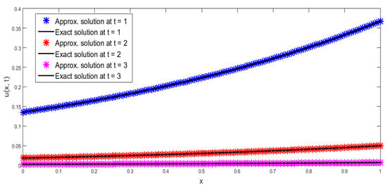
Figure 1. Comparison of approx. and exact profiles at $t$ = 1, 2, 3 regarding Example 1.

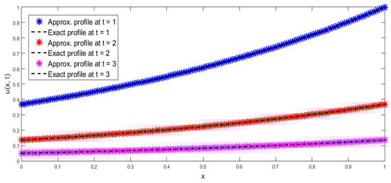
Figure 2. Comparison of approx. and exact profiles at $t$ = 1, 2, 3 regarding Example 2.

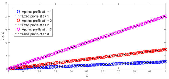
Figure 3. Comparison of approx. and exact profiles at $t$ = 1, 2, 3 regarding Example 3.

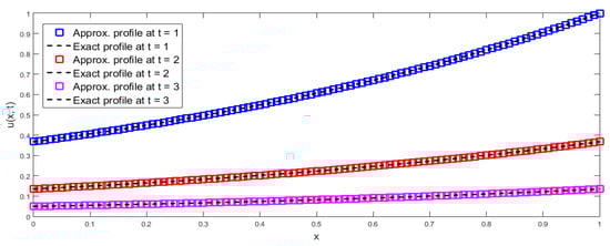
Figure 4. Comparison of approx. and exact profiles at $t$ = 1, 2, 3 regarding Example 4.

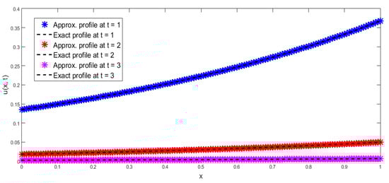
Figure 5. Comparison of approx. and exact profiles at $t$ = 1, 2, 3 regarding Example 5.

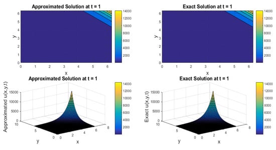
Figure 6. Comparison of approx. and exact profiles at $t$ = 1 regarding Example 6.

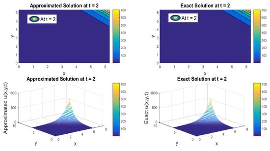
Figure 7. Comparison of approx. and exact profiles at $t$ = 2 regarding Example 6.

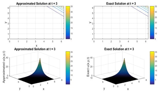
Figure 8. Comparison of approx. and exact profiles at $t$ = 3 regarding Example 6.

In Table 4, the $L_{\infty }$ error was provided at diverse time levels. It is noticeable that at each time level, the obtained error got reduced by increasing the value of $N$, which is a parameter of the convergence of the proposed scheme. In Table 5, $L_{\infty }$ errors were fetched at $t$ = 1.1, 1.2, and 1.3, where, upon increasing the value of $N$, obtained errors got reduced up to ${10}^{-16}$. $L_{\infty }$ errors were obtained at $t$ = 1.1, 1.2, and 1.3, and on changing the value of $N$ from 10 to 20, errors got reduced significantly up to ${10}^{-16}$. In Table 6, the $L_{\infty }$ error was evaluated at $t$ = 1.1, 1.2, and 1.3, upon changed values of $N$, errors got reduced up to ${10}^{-15}$. In Table 7, the $L_{\infty }$ error was calculated at $t$ = 0.1, 0.2, and 0.3; with the change in the value of $N$, the error got reduced up to ${10}^{-11}.$ Therefore, it is affirmed that the proposed regime is generating the convergent solution with a higher and acceptable order of convergence for a wide range of time levels.

Table 4. Error analysis regarding Example 1.

$\mathit{N}$	${\mathit{L}}_{\mathit{\infty }}\mathbf{Error}$
	$t$ = 1	$t$ = 1.3	$t$ = 1.5
10	$1.3701\times {10}^{-3}$	$1.8034\times {10}^{-2}$	$7.3219\times {10}^{-2}$
20	$3.1701\times {10}^{-12}$	$5.8706\times {10}^{-10}$	$1.0099\times {10}^{-8}$
30	$2.2204\times {10}^{-16}$	$-3.4417\times {10}^{-15}$	$7.2164\times {10}^{-16}$
	$\mathrm{Convergence}\mathrm{upto}{10}^{-16}$	$\mathrm{Convergence}\mathrm{upto}{10}^{-15}$	$\mathrm{Convergence}\mathrm{upto}{10}^{-16}$

Table 5. Error analysis regarding Example 2 and 4.

$\mathit{N}$	${\mathit{L}}_{\mathit{\infty }}\mathbf{Error}$
	$t$= 1.1	$t$= 1.2	$t$= 1.3
10	$3.7337\times {10}^{-6}$	$8.8389\times {10}^{-6}$	$1.9517\times {10}^{-5}$
20	$4.4409\times {10}^{-16}$	$4.4409\times {10}^{-16}$	$4.4409\times {10}^{-16}$

Table 6. Error analysis regarding Example 5.

$\mathit{N}$	${\mathit{L}}_{\mathit{\infty }}\mathbf{Error}$
	$t$= 1.1	$t$= 1.2	$t$= 1.3
10	$3.4987\times {10}^{-3}$	$8.2241\times {10}^{-3}$	$1.8034\times {10}^{-2}$
20	$2.1144\times {10}^{-11}$	$1.1944\times {10}^{-10}$	$5.8706\times {10}^{-10}$
30	$1.3323\times {10}^{-15}$	$-1.4433\times {10}^{-15}$	$-3.4417\times {10}^{-15}$

Table 7. Error analysis regarding Example 6.

$\mathit{N}$	${\mathit{L}}_{\mathit{\infty }}\mathbf{Error}$
	$t$= 0.1	$t$= 0.2	$t$= 0.3
10	$4.5419\times {10}^{-7}$	$4.5299\times {10}^{-4}$	$2.5457\times {10}^{-2}$
20	$8.7311\times {10}^{-11}$	$7.2760\times {10}^{-11}$	$4.3656\times {10}^{-11}$

Application of the proposed regime [93].

Considered an infinitesimal piece of the telegraph cable wire as an electrical circuit [Figure 9], and consider that the cable has the perfect insulation, so that the capacitor and leakage to the floor are present. $C$ is the capacitance to the ground; $x$ is the distance from the end of cable; $u\left(x,t\right)$ is the voltage; $G$ is the inductance; $i\left(x,t\right)$ is the current; $L$ is the inductance of the cable.

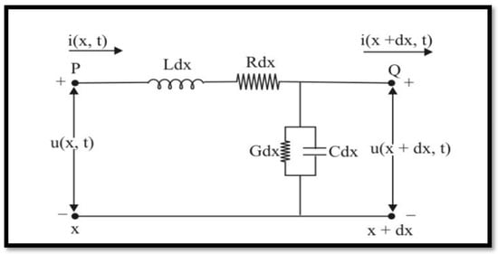
Figure 9. Telegraph transmission line with leakage.

Fractional derivative model equations are [93]:

$$c^2{D}_x^{\delta }i=D_t^{\beta }i+\left(\theta +\varphi \right)D_t^{\alpha }i+\theta \varphi i$$

and

$$c^2{D}_x^{\delta }u=D_t^{\beta }u+\left(\theta +\varphi \right)D_t^{\alpha }u+\theta \varphi u$$

and where $0<\alpha \le 1,1<\delta ,\beta \le 2$.

6. Conclusions

In the present paper, the general formulae are provided to obtain the approximated and exact solutions of the HT equation in 1D, 2D, and 3D using the iterative Shehu transform method. With the aid of graphical representation, it is claimed that a good compatibility of results is obtained for a wide range of time levels. In the tabular discussion, it is noticed that on changing the value of grid points, the obtained $L_{\infty }$ error was reduced up to a high and acceptable order of convergence. With the aid of the tabular form, the convergence of the proposed regime was claimed. The present regime might be one of the most useful regimes to tackle fractional differential equations and partial-integro differential equations.

References

- Ahmadi, S.A.P.; Hosseinzadeh, H.; Cherati, A.Y. A new integral transform for solving higher order linear ordinary Laguerre and Hermite differential equations. Int. J. Appl. Comput. Math. 2019, 5, 142. [Google Scholar] [CrossRef]
- Mahgoub, M.M.A.; Mohand, M. The new integral transform “Sawi Transform”. Adv. Theor. Appl. Math. 2019, 14, 81–87. [Google Scholar]
- Eltayeb, H.; Kılıçman, A.; Fisher, B. A new integral transform and associated distributions. Integral Transform. Spec. Funct. 2010, 21, 367–379. [Google Scholar] [CrossRef]
- Elzaki, T.M. The new integral transform “Elzaki Transform”. Glob. J. Pure Appl. Math. 2011, 7, 57–64. [Google Scholar]
- Kim, H. On the form and properties of an integral transform with strength in integral transforms. Far East J. Math. Sci. 2017, 102, 2831–2844. [Google Scholar] [CrossRef]
- Kim, H. The intrinsic structure and properties of Laplace-typed integral transforms. Math. Probl. Eng. 2017, 2017, 1762729. [Google Scholar] [CrossRef]
- Khan, Z.H.; Khan, W.A. N-transform properties and applications. NUST J. Eng. Sci. 2008, 1, 127–133. [Google Scholar]
- Shah, K.; Junaid, M.; Ali, N. Extraction of Laplace, Sumudu, Fourier and Mellin transform from the natural transform. J. Appl. Environ. Biol. Sci. 2015, 5, 108–115. [Google Scholar]
- Watugala, G. Sumudu transform: A new integral transform to solve differential equations and control engineering problems. Integr. Educ. 1993, 24, 35–43. [Google Scholar] [CrossRef]
- Kapoor, M. Exact solution of coupled 1D non-linear Burgers’ equation by using Homotopy Perturbation Method (HPM): A review. J. Phys. Commun. 2020, 4, 095017. [Google Scholar] [CrossRef]
- Baleanu, D.; Wu, G.C. Some further results of the laplace transform for variable–order fractional difference equations. Fract. Calc. Appl. Anal. 2019, 22, 1641–1654. [Google Scholar] [CrossRef]
- Bokhari, A. Application of Shehu transform to Atangana-Baleanu derivatives. J. Math. Comput. Sci. 2019, 20, 101–107. [Google Scholar] [CrossRef]
- Chand, M.; Hammouch, Z. Unified fractional integral formulae involving generalized multiindex Bessel function. In Proceedings of the International Conference on Computational Mathematics and Engineering Sciences, Antalya, Turkey, 20–22 April 2019; pp. 278–290. [Google Scholar]
- Cho, I.; Kim, H. The solution of Bessel’s equation by using integral transforms. Appl. Math. Sci. 2013, 7, 6069–6075. [Google Scholar] [CrossRef]
- Elzaki, T.M. Elzaki and Sumudu transforms for solving some differential equations. Glob. J. Pure Appl. Math. 2012, 8, 167–173. [Google Scholar]
- Shah, N.A.; Hamed, Y.S.; Abualnaja, K.M.; Chung, J.-D.; Shah, R.; Khan, A. A Comparative Analysis of Fractional-Order Kaup–Kupershmidt Equation within Different Operators. Symmetry 2022, 14, 986. [Google Scholar] [CrossRef]
- Sweilam, N.H.; Al-Mekhlafi, S.M.; Baleanu, D. Nonstandard finite difference method for solving complex-order fractional Burgers’ equations. J. Adv. Res. 2020, 25, 19–29. [Google Scholar] [CrossRef]
- Abbas, N.; Malik, M.Y.; Alqarni, M.S.; Nadeem, S. Study of three dimensional stagnation point flow of hybrid nanofluid over an isotropic slip surface. Phys. A Stat. Mech. Appl. 2020, 554, 124020. [Google Scholar] [CrossRef]
- Ali, U.; Malik, M.Y.; Rehman, K.U.; Alqarni, M.S. Exploration of cubic autocatalysis and thermal relaxation in a non-Newtonian flow field with MHD effects. Phys. A Stat. Mech. Appl. 2020, 549, 124349. [Google Scholar] [CrossRef]
- Khan, M.; Salahuddin, T.; Malik, M.Y.; Alqarni, M.S.; Alqahtani, A.M. Numerical modeling and analysis of bioconvection on MHD flow due to an upper paraboloid surface of revolution. Phys. A Stat. Mech. Appl. 2020, 553, 124231. [Google Scholar] [CrossRef]
- Shah, N.A.; Agarwal, P.; Chung, J.D.; El-Zahar, E.R.; Hamed, Y.S. Analysis of Optical Solitons for Nonlinear Schrödinger Equation with Detuning Term by Iterative Transform Method. Symmetry 2020, 12, 1850. [Google Scholar] [CrossRef]
- Singh, J.; Kumar, D.; Baleanu, D.; Rathore, S. An efficient numerical algorithm for the fractional Drinfeld–Sokolov–Wilson equation. Appl. Math. Comput. 2018, 335, 12–24. [Google Scholar] [CrossRef]
- Shah, N.A.; Dassios, I.; Chung, J.D. A decomposition method for a fractional-order multi-dimensional telegraph equation via the Elzaki transform. Symmetry 2020, 13, 8. [Google Scholar] [CrossRef]
- He, W.; Chen, N.; Dassios, I.; Shah, N.A.; Chung, J.D. Fractional system of Korteweg-De Vries equations via Elzaki transform. Mathematics 2021, 9, 673. [Google Scholar] [CrossRef]
- Kapoor, M. Sumudu transform HPM for Klein-Gordon and Sine-Gordon equations in one dimension from an analytical aspect. J. Math. Comput. Sci. 2022, 12, 93. [Google Scholar] [CrossRef]
- Kapoor, M.; Joshi, V. Comparison of Two Hybrid Schemes Sumudu HPM and Elzaki HPM for Convection-Diffusion Equation in Two and Three Dimensions. Int. J. Appl. Comput. Math. 2022, 8, 110. [Google Scholar] [CrossRef]
- Shah, N.A.; Imran, M.A.; Miraj, F. Exact Solutions of Time Fractional free Convection flows of viscous fluid over an IsoThermal vertical plate with Caputo and Caputo-Fabrizio derivatives. J. Prime Res. Math. 2017, 13, 57–64. [Google Scholar]
- Shah, N.A.; Agarwal, P.; Chung, J.D.; Althobaiti, S.; Sayed, S.; Aljohani, A.; Alkafafy, M. Analysis of time-fractional Burgers and Diffusion Equations by using Modified q-HATM. Fractals 2021, 30, 2240012. [Google Scholar] [CrossRef]
- Akinyemi, L.; Veeresha, P.; Ajibola, S.O. Numerical simulation for coupled nonlinear Schrödinger–Korteweg–de Vries and Maccari systems of equations. Mod. Phys. Lett. B 2021, 35, 2150339. [Google Scholar] [CrossRef]
- Prakash, A.; Veeresha, P.; Prakasha, D.G.; Goyal, M. A homotopy technique for a fractional order multi-dimensional telegraph equation via the Laplace transform. Eur. Phys. J. Plus 2019, 134, 19. [Google Scholar] [CrossRef]
- Elzaki, T.M.; Biazar, J. Homotopy perturbation method and Elzaki transform for solving system of nonlinear partial differential equations. World Appl. Sci. J. 2013, 24, 944–948. [Google Scholar]
- Elzaki, T.M. On the Elzaki transform and higher order ordinary differential equations. Adv. Theor. Appl. Math. 2011, 6, 107–113. [Google Scholar]
- Elzaki, T.M.; Hilal, E.M.; Arabia, J.S.; Arabia, J.S. Homotopy perturbation and Elzaki transform for solving nonlinear partial differential equations. Math. Theory Modeling 2012, 2, 33–42. [Google Scholar]
- Verma, D.; Alam, A. Analysis of Simultaneous Differential Equations by Elzaki Transform Approach. Sci. Technol. Dev. 2020, 9, 364–367. [Google Scholar]
- Elzaki, T.M. On the Elzaki transforms and system of partial diffrential equations. Adv. Theor. Applid Math. 2011, 1, 115–123. [Google Scholar]
- Elzaki, T.M.; Hilal, E.M.A. Analytical solution for telegraph equation by modified of Sumudu transform “Elzaki transform”. Math. Theory Model. 2012, 2, 104–111. [Google Scholar]
- Song, Y.; Kim, H. The solution of Volterra integral equation of the second kind by using the Elzaki transform. Appl. Math. Sci. 2014, 8, 525–530. [Google Scholar] [CrossRef]
- Belgacem, F.B.M.; Karaballi, A.A. Sumudu transform fundamental properties investigations and applications. Int. J. Stoch. Anal. 2006, 2006, 91083. [Google Scholar] [CrossRef]
- Bulut, H.; Baskonus, H.M.; Belgacem, F.B.M. The analytical solution of some fractional ordinary differential equations by the Sumudu transform method. Abstr. Appl. Anal. 2013, 2013, 203875. [Google Scholar] [CrossRef]
- Kılıçman, A.; Gadain, H.E. On the applications of Laplace and Sumudu transforms. J. Frankl. Inst. 2010, 347, 848–862. [Google Scholar] [CrossRef]
- Tuluce Demiray, S.; Bulut, H.; Belgacem, F.B.M. Sumudu transform method for analytical solutions of fractional type ordinary differential equations. Math. Probl. Eng. 2015, 2015, 131690. [Google Scholar] [CrossRef]
- Kiliçman, A.; Eltayeb, H.; Agarwal, R.P. On Sumudu transform and system of differential equations. Abstr. Appl. Anal. 2010, 2010, 598702. [Google Scholar] [CrossRef]
- Singh, J.; Kumar, D.; Sushila, D. Homotopy perturbation Sumudu transform method for nonlinear equations. Adv. Theor. Appl. Mech. 2011, 4, 165–175. [Google Scholar]
- Eltayeb, H.; Kılıçman, A. A note on the Sumudu transforms and differential equations. Appl. Math. Sci. 2010, 4, 1089–1098. [Google Scholar]
- Yousif, E.A.; Hamed, S.H. Solution of nonlinear fractional differential equations using the homotopy perturbation Sumudu transform method. Appl. Math. Sci. 2014, 8, 2195–2210. [Google Scholar] [CrossRef]
- Hamza, A.E.; Elzaki, T.M. Application of Homotopy perturbation and Sumudu transform method for solving Burgers equations. Am. J. Theor. Appl. Stat. 2015, 4, 480–483. [Google Scholar] [CrossRef]
- Rawashdeh, M.S.; Maitama, S. Solving coupled system of nonlinear PDE’s using the natural decomposition method. Int. J. Pure Appl. Math. 2014, 92, 757–776. [Google Scholar] [CrossRef]
- Rawashdeh, M.S.; Maitama, S. Solving nonlinear ordinary differential equations using the NDM. J. Appl. Anal. Comput. 2015, 5, 77–88. [Google Scholar]
- Belgacem, F.B.M.; Silambarasan, R. Theory of natural transform. Math. Eng. Sci. Aerosp. 2012, 3, 99–124. [Google Scholar]
- Maitama, S. A hybrid natural transform homotopy perturbation method for solving fractional partial differential equations. Int. J. Differ. Equ. 2016, 2016, 9207869. [Google Scholar] [CrossRef]
- Alkaleeli, S.R.; Mtawal, A.A.; Hmad, M.S. Triple Shehu transform and its properties with applications. Afr. J. Math. Comput. Sci. Res. 2021, 14, 4–12. [Google Scholar]
- Sunthrayuth, P.; Shah, R.; Zidan, A.M.; Khan, S.; Kafle, J. The Analysis of Fractional-Order Navier-Stokes Model Arising in the Unsteady Flow of a Viscous Fluid via Shehu Transform. J. Funct. Spaces 2021, 2021, 1029196. [Google Scholar] [CrossRef]
- Areshi, M.; Zidan, A.M.; Shah, R.; Nonlaopon, K. A Modified Techniques of Fractional-Order Cauchy-Reaction Diffusion Equation via Shehu Transform. J. Funct. Spaces 2021, 2021, 5726822. [Google Scholar] [CrossRef]
- Qureshi, S.; Kumar, P. Using Shehu integral transform to solve fractional order Caputo type initial value problems. J. Appl. Math. Comput. Mech. 2019, 18, 75–83. [Google Scholar] [CrossRef]
- Chu, Y.M.; Bani Hani, E.H.; El-Zahar, E.R.; Ebaid, A.; Shah, N.A. Combination of Shehu decomposition and variational iteration transform methods for solving fractional third order dispersive partial differential equations. Numer. Methods Partial. Differ. Equ. 2021. [Google Scholar] [CrossRef]
- Cetinkaya, S.; Demir, A.; Sevindir, H.K. Solution of Space-Time-Fractional Problem by Shehu Variational Iteration Method. Adv. Math. Phys. 2021, 2021, 5528928. [Google Scholar] [CrossRef]
- Akinyemi, L.; Iyiola, O.S. Exact and approximate solutions of time-fractional models arising from physics via Shehu transform. Math. Methods Appl. Sci. 2020, 43, 7442–7464. [Google Scholar] [CrossRef]
- Higazy, M.; Aggarwal, S.; Nofal, T.A. Sawi Decomposition Method for Volterra Integral Equation with Application. J. Math. 2020, 2020, 6687134. [Google Scholar] [CrossRef]
- Aggarwal, S.; Sharma, S.D.; Vyas, A. Sawi Transform of Bessel’s Functions with Application for Evaluating Definite Integrals. Int. J. Latest Technol. Eng. Manag. Appl. Sci. 2020, 9, 12–18. [Google Scholar]
- Singh, G.P.; Aggarwal, S. Sawi transform for population growth and decay problems. Int. J. Latest Technol. Eng. Manag. Appl. Sci. 2019, 8, 157–162. [Google Scholar]
- Higazy, M.; Aggarwal, S. Sawi transformation for system of ordinary differential equations with application. Ain Shams Eng. J. 2021, 12, 3173–3182. [Google Scholar] [CrossRef]
- Ahmadi, S.P.; Hosseinzadeh, H.; Cherati, A.Y. A New IntegralTransform for Solving Higher OrderOrdinary Differential Equations. Nonlinear Dyn. Syst. Theory 2019, 19, 243252. [Google Scholar]
- Saadeh, R.; Qazza, A.; Burqan, A. A new integral transform: Ara transform and its properties and applications. Symmetry 2020, 12, 925. [Google Scholar] [CrossRef]
- Eltayeb, H.; Kılıçman, A. A note on solutions of wave, Laplace’s and heat equations with convolution terms by using a double Laplace transform. Appl. Math. Lett. 2008, 21, 1324–1329. [Google Scholar] [CrossRef]
- Bhanotar, S.A.; Kaabar, M.K. Analytical solutions for the nonlinear partial differential equations using the conformable triple Laplace transform decomposition method. Int. J. Differ. Equ. 2021, 2021, 9988160. [Google Scholar] [CrossRef]
- Debnath, L. The double Laplace transforms and their properties with applications to functional, integral and partial differential equations. Int. J. Appl. Comput. Math. 2016, 2, 223–241. [Google Scholar] [CrossRef]
- Shaikh, S.L. Introducing a new integral transform: Sadik Transform. Am. Int. J. Res. Sci. Technol. Eng. Math. 2018, 22, 100–102. [Google Scholar]
- Shaikh, S.L. Sadik transform in control theory. Int. J. Innov. Sci. Res. Technol. 2018, 3, 396–398. [Google Scholar]
- Redhwan, S.S.; Shaikh, S.L.; Abdo, M.S. On a study of some new results in fractional calculus through Sadik transform. Our Herit. 2020, 68, 12. [Google Scholar]
- Redhwan, S.S.; Shaikh, S.L.; Abdo, M.S.; Al-Mayyahi, S.Y. Sadik transform and some result in fractional calculus. Malaya J. Mat. MJM 2020, 8, 536–543. [Google Scholar] [CrossRef]
- Maitama, S.; Zhao, W. New integral transform: Shehu transform a generalization of Sumudu and Laplace transform for solving differential equations. arXiv 2019, arXiv:1904.11370. [Google Scholar]
- Leibniz, G.W. Letter from Hanover, Germany to GFA L’Hospital, September 30, 1695. Math. Schr. 1849, 2, 301–302. [Google Scholar]
- Leibniz, G.W. Letter from Hanover, Germany to Johann Bernoulli, December 28, 1695. In Leibniz Mathematische Schriften; OlmsVerlag: Hildesheim, Germany, 1962; p. 226. [Google Scholar]
- Podlubny, I. Fractional Differential Equations: An Introduction to Fractional Derivatives, Fractional Differential Equations, to Methods of Their Solution and Some of Their Applications; Elsevier: Amsterdam, The Netherlands, 1998. [Google Scholar]
- Sun, H.; Zhang, Y.; Baleanu, D.; Chen, W.; Chen, Y. A new collection of real world applications of fractional calculus in science and engineering. Commun. Nonlinear Sci. Numer. Simul. 2018, 64, 213–231. [Google Scholar] [CrossRef]
- Chen, D.; Chen, Y.; Xue, D. Three fractional-order TV-L2 models for image denoising. J. Comput. Inf. Syst. 2013, 9, 4773–4780. [Google Scholar]
- Ullah, A.; Chen, W.; Khan, M.A.; Sun, H. An efficient variational method for restoring images with combined additive and multiplicative noise. Int. J. Appl. Comput. Math. 2017, 3, 1999–2019. [Google Scholar] [CrossRef]
- Hilfer, R.; Anton, L. Fractional master equations and fractal time random walks. Phys. Rev. E 1995, 51, R848. [Google Scholar] [CrossRef]
- Mainardi, F. Fractional Calculus and Waves in Linear Viscoelasticity: An Introduction to Mathematical Models; Imperial College Press: London, UK, 2010. [Google Scholar]
- Xue, D.; Monje, C.A.; Feliu, V.; Vinagre, B.M.; Chen, Y. Fractional-order Systems and Controls: Fundamentals and Applications. In Advances in Industrial Control; Springer: Berlin/Heidelberg, Germany, 2010. [Google Scholar]
- Yang, X.J.; Srivastava, H.M.; Machado, J.A.T. A new fractional derivative without singular kernel: Application to the modelling of the steady heat flow. arXiv 2016, arXiv:1601.01623. [Google Scholar] [CrossRef]
- Zhang, J.; Wei, Z.; Xiao, L. Adaptive fractional-order multi-scale method for image denoising. J. Math. Imaging Vis. 2012, 43, 39–49. [Google Scholar] [CrossRef]
- Zhang, Y.; Pu, Y.F.; Hu, J.R.; Zhou, J.L. A class of fractional-order variational image inpainting models. Appl. Math. Inf. Sci. 2012, 6, 299–306. [Google Scholar]
- Yi-Fei, P.U. Fractional differential analysis for texture of digital image. J. Algorithms Comput. Technol. 2007, 1, 357–380. [Google Scholar] [CrossRef]
- Singh, B.K.; Kumar, P. Numerical computation for time-fractional gas dynamics equations by fractional reduced differential transforms method. J. Math. Syst. Sci. 2016, 6, 248–259. [Google Scholar]
- Singh, J.; Kumar, D.; Swroop, R. Numerical solution of time-and space-fractional coupled Burgers’ equations via homotopy algorithm. Alex. Eng. J. 2016, 55, 1753–1763. [Google Scholar] [CrossRef]
- Ragab, A.A.; Hemida, K.M.; Mohamed, M.S.; Abd El Salam, M.A. Solution of time-fractional Navier–Stokes equation by using homotopy analysis method. Gen. Math. Notes 2012, 13, 13–21. [Google Scholar]
- Chen, Y.; An, H.L. Numerical solutions of coupled Burgers equations with time-and space-fractional derivatives. Appl. Math. Comput. 2008, 200, 87–95. [Google Scholar] [CrossRef]
- Saravanan, A.; Magesh, N. A comparison between the reduced differential transform method and the Adomian decomposition method for the Newell–Whitehead–Segel equation. J. Egypt. Math. Soc. 2013, 21, 259–265. [Google Scholar] [CrossRef]
- Singh, B.K.; Srivastava, V.K. Approximate series solution of multi-dimensional, time fractional-order (heat-like) diffusion equations using FRDTM. R. Soc. Open Sci. 2015, 2, 140511. [Google Scholar] [CrossRef]
- Singh, B.K.; Kumar, P. FRDTM for numerical simulation of multi-dimensional, time-fractional model of Navier–Stokes equation. Ain Shams Eng. J. 2018, 9, 827–834. [Google Scholar] [CrossRef]
- Prakash, A.; Kumar, M.; Sharma, K.K. Numerical method for solving fractional coupled Burgers equations. Appl. Math. Comput. 2015, 260, 314–320. [Google Scholar] [CrossRef]
- Khan, H.; Shah, R.; Baleanu, D.; Kumam, P.; Arif, M. Analytical solution of fractional-order hyperbolic telegraph equation, using natural transform decomposition method. Electronics 2019, 8, 1015. [Google Scholar] [CrossRef]
- Eltayeb, H.; Abdalla, Y.T.; Bachar, I.; Khabir, M.H. Fractional telegraph equation and its solution by natural transform decomposition method. Symmetry 2019, 11, 334. [Google Scholar] [CrossRef]
- Momani, S. Analytic and approximate solutions of the space-and time-fractional telegraph equations. Appl. Math. Comput. 2005, 170, 1126–1134. [Google Scholar] [CrossRef]
Publisher’s Note: MDPI stays neutral with regard to jurisdictional claims in published maps and institutional affiliations. |
© 2022 by the authors. Licensee MDPI, Basel, Switzerland. This article is an open access article distributed under the terms and conditions of the Creative Commons Attribution (CC BY) license (https://creativecommons.org/licenses/by/4.0/).