Article

Two-Step Neural-Network-Based Fault Isolation for Stochastic Systems

1
Shoool of Ationautom, Nanjing University of Information Science & Techonlogy, Nanjing 210044, China
2
Jiangsu Collaborative Innovation Center on Atmospheric Environment and Equipment Technology, Nanjing 210044, China
3
School of Information, North China University of Technology, Langfang 065000, China
*
Author to whom correspondence should be addressed.
Mathematics 2022, 10(22), 4261; https://doi.org/10.3390/math10224261 (registering DOI)
Submission received: 12 October 2022 / Revised: 30 October 2022 / Accepted: 11 November 2022 / Published: 14 November 2022
(This article belongs to the Special Issue Dynamic Modeling and Simulation for Control Systems)

Abstract

:
This paper studies a fault isolation method for an optical fiber vibration source detection and early warning system. We regard the vibration sources in the system as faults and then detect and isolate the faults of the system based on a two-step neural network. Firstly, the square root B-spline expansion method is used to approximate the output probability density functions. Secondly, the nonlinear weight dynamic model is established through a dynamic neural network. Thirdly, the nonlinear filter and residual generator are constructed to estimate the weight, analyze the residual, and estimate the threshold, so as to detect, diagnose, and isolate the faults. The feasibility criterion of fault detection and isolation is given by using some linear matrix inequalities, and the stability of the estimation error system is proven according to the Lyapunov theorem. Finally, simulation experiments based on a optical fiber vibration source system are given to verify the effectiveness of this method.

1. Introduction

With the development of industrial automation, the scale and complexity of modern control systems are increasing rapidly. During operation, the sensor, actuator, and some components might fail due to aging, wearing, or other reasons [1,2,3,4]. If the faults of the system cannot be detected and eliminated in time in the process of operation, this may lead to system failure, paralysis, and even catastrophic consequences [5]. Therefore, in the past few decades, the theory of fault detection and isolation (FDI) has developed rapidly [6,7,8,9,10].
The purpose of fault detection and isolation is that, when multiple faults occur in the system, we can find and isolate these faults in time and estimate the size of each fault [6]. At present, many research achievements have been made in fault detection and fault isolation [11,12,13,14,15,16,17]. Classical fault detection and isolation methods include the T-S fuzzy model [11], the independent component analysis fault isolation method [12], the detection filter method [13], minimum variance fault estimation [14], etc.
In fact, actual industrial systems are stochastic systems [18,19,20,21]. Due to the nonlinearity of the system, even if the input obeys a Gaussian distribution, the output of the system will also obey a non-Gaussian distribution [18]. At present, there are many research results that focus on fault diagnosis and isolation for stochastic distribution systems. For example, in [8], an adaptive fault diagnosis observer was used to diagnose actuator faults and accurately estimate the fault size. In [19], fault diagnosis schemes for stochastic distributed systems were studied based on the minimum entropy principle. In [20], a fault isolation method based on entropy optimization filtering was studied for nonlinear non-Gaussian systems with unmeasurable outputs.
As we know, in order to monitor the operation of oil or gas pipelines, a commonly used method is to embed the oil or gas pipelines together with optical fibers in the same ditch. The conditions of the oil or gas pipelines can be monitored by observing the optical fiber’s output data in one end of the fiber if we input light at the other end [22,23,24]. However, In the optical fiber vibration source detection and early warning system, the sensors are quite sensitive due to inevitable non-stationary interferences from the environment, which often brings false alarms. To reduce the false alarm rate, we regard the vibration sources, such as pickaxe planing of mechanical excavation, as faults, and the objective is then transferred into detecting and isolating the faults. Different from the literature in the optical fiber vibration source detection field [22,23], we use a two-step neural network to model the optic data collected from the end of the fiber. The false alarm rate is controlled below the threshold, and the different vibration sources are estimated and isolated by using filter designing, convex optimization, Lyapunov theorems, etc.
This paper is organized as follows: In Section 2, the static modeling is carried out with the help of square root B-splines, and the nonlinear weighted dynamic model is established through the neural network to describe the FDI problem. In Section 3, based on the adaptive filter, the fault detection problem of the transformed nonlinear weighted dynamic model is studied. In Section 4, according to the adaptive fault diagnosis method, the size of different faults is estimated to achieve the purpose of fault isolation. The simulation is given in Section 5 to illustrate the feasibility of the results.

2. Static Modeling and Weighted Dynamic Modeling

For the optical fiber vibration source detection system, although the output value cannot be measured directly, the output PDFs can be estimated by the kernel density method [23]. Next, the output PDF at each sampling time is approximated by B-splines, and the weight of each B-splines is calculated.

2.1. Output PDFs’ Static Modeling

As in Figure 1, let u ( t ) R m be the input of the nonlinear stochastic optical fiber vibration detection system, y ( t ) [ a , b ] be the output light intensity, F 1 and F 2 be the fault vectors (vibration sources) to be detected and diagnosed, and the probability distribution of the output y ( t ) of the stochastic dynamic system in the interval [ a , ξ ] satisfy the condition P ( a y ( t ) ξ ) = a ξ γ ( z , u ( t ) , F 1 , F 2 ) d z . We can use the square root B-spline model with approximate error as shown in (1) to statically model the output PDFs [8]:
γ ( z , u ( t ) , F 1 , F 2 ) = i = 1 n v i ( u ( t ) , F 1 , F 2 ) b i ( z ) + ω 0 ( z , u ( t ) , F 1 , F 2 )
where v i ( u ( t ) , F 1 , F 2 ) ( i = 1 , 2 , , n ) are the corresponding weights of B-spline expansion and b i ( z ) ( i = 1 , 2 , , n ) are the pre-specified basis functions on interval [ a , b ] . For all { z , u ( t ) , F 1 , F 2 } , the term ω 0 ( z , u ( t ) , F 1 , F 2 ) represents the model uncertainty or the error term on the approximation of the PDFs, which is supposed to satisfy | ω 0 ( z , u ( t ) , F 1 , F 2 ) | δ 0 , where δ 0 is assumed to be a known positive number. Denote
B ( z ) = [ b 1 ( z ) , b 2 ( z ) , , b n 1 ( z ) ]
V ( t ) = [ v 1 ( u ( t ) , F 1 , F 2 ) , v 2 ( u ( t ) , F 1 , F 2 ) , , v n 1 ( u ( t ) , F 1 , F 2 ) ]
and
Λ 1 = a b B T ( z ) B ( z ) d z
Λ 2 = a b B T ( z ) b n ( z ) d z
Λ 3 = a b ( b n ) 2 ( z ) d z
where Λ 1 R ( n 1 ) × ( n 1 ) , Λ 2 R ( n 1 ) × 1 , and Λ 3 R 1 × 1 are known matrices or constants. In the following, for simplicity, V ( u ( t ) , F 1 , F 2 ) is written as V ( t ) . According to the properties of the probability density function, for any γ ( z , u ( t ) , F 1 , F 2 ) , the constraint condition a ξ γ ( z , u ( t ) , F 1 , F 2 ) d z = 1 is always true, and only n 1 weight vectors in the weight { v i ( u ( t ) , F 1 , F 2 ) : i = 1 , 2 , , n } are independent. Let Λ 0 = Λ 1 Λ 3 Λ 2 T Λ 2 , then the following inequality holds [8]:
( 1 ω 1 ( z , u ( t ) , F 1 , F 2 ) ) Λ 3 V T ( t ) V ( t ) 0
where
ω 1 z , u t , F 1 , F 2 = 2 ω 0 2 z , u t , F 1 , F 2 × a b B z d z V t + a b b n z d z v n t + ω 0 2 z , u t , F 1 , F 2 b a
From (5), we can obtain:
V T ( t ) Λ 0 V ( t ) 1 ω 1 z , u t , F 1 , F 2 Λ 3
where
Λ 0 > 0 , 1 ω 1 z , u t , F 1 , F 2 > 0
According to (6), we can know V ( t ) is bounded and V ( t ) 2 δ ˜ = Λ 0 1 Λ 3 holds. Therefore, (1) can be rewritten as:
γ ( z , u t , F 1 , F 2 ) = B z V t + h 0 ( V t , ω 1 ) B n ( z )
where h 0 ( V ( t ) , ω 1 ) is a function of V ( t ) and ω 1 ( z , u ( t ) , F 1 , F 2 ) , as shown in (9):
h 0 V t , ω 1 = 1 Λ 3 1 ω 1 Λ 3 V T ( t ) Λ 0 V ( t ) Λ 2 V t Λ 3
In order to simplify the B-spline model represented by (8), h 0 ( V ( t ) , ω 1 ) can be further approximated as:
γ ( z , u ( t ) , F 1 , F 2 ) = B ( z ) V ( t ) + h ( V ( t ) ) b n ( z ) + ω ( z , u ( t ) , F 1 , F 2 )
Equation (10) is a nonlinear output equation with uncertainty, and the term h ( V ( t ) ) satisfies
h ( V ( t ) ) = 1 Λ 3 ( Λ 2 ± Λ 3 V T ( t ) Λ 0 V ( t ) )
As V ( t ) is bounded and ω 0 ( z , u ( t ) , F 1 , F 2 ) δ 0 , it can be concluded that ω ( z , u ( t ) , F 1 , F 2 ) δ holds for all { z , u ( t ) , F 1 , F 2 } . For h ( V ( t ) ) in (11), it is supposed that, for any V 1 ( t ) and V 2 ( t ) , there exists a known matrix U 1 , such that:
h ( V 1 ( t ) ) h ( V 2 ( t ) ) U 1 ( V 1 ( t ) V 2 ( t ) )

2.2. Nonlinear Dynamic Weight Model

After the B-spline expansion of the output PDFs, the next task is to find the dynamic relationship between u ( t ) and γ . As V ( t ) is a nonlinear function of u ( t ) , we perform the modeling with the help of a neural network as in [25] and study the following weight dynamic system:
x ˙ ( t ) = A x ( t ) + G g ( x ( t ) ) + H u ( t ) + F 1 + F 2 V ( t ) = D x ( t )
where x ( t ) R m is the state vector, A, G, H, and D represent the known parameter matrices, and g ( x ( t ) ) is a nonlinear function. Supposing g ( 0 ) = 0 and for any x 1 ( t ) , x 2 ( t ) , the following inequality holds [8]:
g ( x 1 ( t ) ) g ( x 2 ( t ) ) U 2 ( x 1 ( t ) x 2 ( t ) )
where U 2 is a known matrix. According to (13), (10) can be rewritten as:
γ ( z , u t , F 1 , F 2 ) = B z D x t + h D x t b n z + ω ( z , u t , F 1 , F 2 )
Because there exist nonlinear terms in the weighted dynamic system, the design of the nonlinear filter is the key in the process of fault detection and isolation. In this paper, the fault detection and fault diagnosis filters are designed, respectively, according to u ( t ) , as well as the output PDFs γ ( z , u t , F 1 , F 2 ) , so as to achieve the task of fault isolation.

3. Fault Detection Filter Design

In order to detect the faults based on the changes of the output PDFs, we construct the following nonlinear filter:
x ^ ˙ ( t ) = A x ^ ( t ) + G g ( x ^ ( t ) ) + H u ( t ) + L ε ( t ) ε ( t ) = a b σ ( z ) [ γ ( z , u ( t ) , F 1 , F 2 ) γ ^ ( z , u ( t ) ) ] d z γ ^ ( z , u ( t ) ) = B ( z ) D x ^ ( t ) + h ( D x ^ ( t ) ) b n ( z )
where x ^ ( t ) is the estimated value of the state vector x ( t ) , L R m × p is the gain of the detection observer to be determined, σ ( z ) R p × 1 is the pre-specified weighting vector defined on [ a , b ] , and the residual ε ( t ) represents the integral of the difference between the measured PDFs γ ( z , u t , F 1 , F 2 ) and the estimated PDFs γ ^ ( z , u ( t ) ) [26]. Denote e ( t ) = x ( t ) x ^ ( t ) , then the first derivative of e ( t ) with respect to time t is:
e ˙ ( t ) = x ˙ ( t ) x ^ ˙ ( t ) = ( A L Γ 1 ) e ( t ) + [ G g ( x ( t ) ) G g ( x ^ ( t ) ) ] L Γ 2 [ h ( D x ( t ) ) h ( D x ^ ( t ) ) ] + F 1 + F 2 L Δ ( t )
where
Γ 1 = a b σ ( z ) B ( z ) d z Γ 2 = a b σ ( z ) b n ( z ) d z Δ ( t ) = a b σ ( z ) ω ( z , u ( t ) , F 1 , F 2 ) d z
As shown in (10) and (16), it is clear that the residual ε ( t ) is a nonlinear function of e ( t ) , x ( t ) , and x ^ ( t ) . According to (18), the residual ε ( t ) can be further expressed as
ε ( t ) = a b σ ( z ) B ( z ) D e ( t ) d z + a b σ ( z ) [ h ( D x ( t ) ) h ( D x ^ ( t ) ) ] b n ( z ) d z + a b σ ( z ) ω ( z , u ( t ) , F 1 , F 2 ) d z = Γ 1 e ( t ) + Γ 2 [ h ( D x ( t ) ) h ( D x ^ ( t ) ) ] + Δ ( t )
Recall ω ( z , u ( t ) , F 1 , F 2 ) < δ , and combine it with (18); we can obtain that
Δ ( t ) < δ ˜
where δ ˜ = δ a b σ ( z ) d z . In (16), σ ( z ) can be any constant vector, and it is required that ( A , Γ 1 ) is observable. In the fault detection stage, according to Theorem 1 in [8], if there exist parameters λ i ( i = 1 , 2 ) , matrices P > 0 , R, and constant η > 0 , then if F 1 = F 2 = 0 , the system (17) with gain L = P 1 R is stable, and the error satisfies:
e ( t ) α 0 = max e ( 0 ) , 2 η 1 δ ˜ R
In order to detect the faults, we select ε ( t ) as the residual signal. According to [8], the faults can be detected as follows:
ε ( t ) > α = α 0 ( Γ 1 + Γ 2 U 1 ) + δ ˜

4. Fault Isolation Filter Design

Once the faults are detected according to the method in Section 2, it is necessary to carry out fault diagnosis and estimate the size of different faults, respectively, so as to achieve fault isolation. For this purpose, we construct the following adaptive filter as shown in (23):
x ^ ˙ ( t ) = A x ^ ( t ) + G g ( x ^ ( t ) ) + H u ( t ) + 1 1 F ^ 1 F ^ 2 + L ε ( t ) F ^ ˙ 1 F ^ ˙ 2 = Λ 5 0 0 Λ 7 F ^ 1 F ^ 2 + Λ 6 Λ 8 ε ( t ) ε ( t ) = a b σ ( z ) [ γ ( z , u ( t ) , F 1 , F 2 ) γ ^ ( z , u ( t ) ) ] d z γ ^ ( z , u ( t ) ) = B ( z ) D x ^ ( t ) + h ( D x ^ ( t ) ) b n ( z )
where F ^ 1 and F ^ 2 are the estimates of faults F 1 and F 2 . In (23), Λ i ( i = 5 , 6 , 7 , 8 ) is the learning operator with respect to F ^ 1 , F ^ 2 , and the fault estimation errors.
Let e ( t ) = x ( t ) x ^ ( t ) , and define the fault estimation errors as F ˜ 1 = F 1 F ^ 1 , F ˜ 2 = F 2 F ^ 2 , then the estimation errors can be shown as in (24):
e ˙ ( t ) = ( A L Γ 1 ) e ( t ) + [ G g ( x ( t ) ) G g ( x ^ ( t ) ) ] L Γ 2 [ h ( D x ( t ) ) h ( D x ^ ( t ) ) ] + F ˜ 1 + F ˜ 2 L Δ ( t ) F ˜ ˙ 1 = Λ 5 F ˜ 1 + Λ 5 F 1 Λ 6 ε ( t ) F ˜ ˙ 2 = Λ 7 F ˜ 2 + Λ 7 F 2 Λ 8 ε ( t ) ε ( t ) = Γ 1 e ( t ) + Γ 2 [ h ( D x ( t ) ) h ( D x ^ ( t ) ) ] + Δ ( t )
Supposing F 1 M 1 / 2 , F 2 M 2 / 2 , the following theorem will show that, by selecting the appropriate filter gains Λ 5 , Λ 6 , Λ 7 , and Λ 8 , the fault estimation errors can be controlled in a small range.
Theorem 1. 
If there exist λ i > 0 ( i = 1 , 2 ) , matrices P > 0 , R, and Λ i ( i = 5 , 6 , 7 , 8 ) , and constants κ > 0 , θ 1 > 0 , θ 2 > 0 , and θ 3 satisfying:
Π 0 + κ I P Γ 1 T Λ 6 T P Γ 1 T Λ 8 T Π 2 0 0 D T U 1 T P Λ 6 Γ 1 2 Λ 5 T 0 0 Π 3 0 0 P Λ 8 Γ 1 0 2 Λ 7 T 0 0 Π 4 0 Π 2 T 0 0 I 0 0 0 0 Π 3 T 0 0 I 0 0 0 0 Π 4 T 0 0 I 0 U 1 D 0 0 0 0 0 1 2 θ 3 2 I < 0
where
Π 2 = [ λ 1 R Γ 2 λ 2 P G θ 1 R ] Π 3 = [ θ 2 Λ 6 θ 3 Λ 6 Γ 2 ] Π 4 = [ θ 2 Λ 8 θ 3 Λ 8 Γ 2 ] Π 0 = ( P A R Γ 1 ) + ( P A R Γ 1 ) T + 1 λ 1 2 D T U 1 T U 1 D + 1 λ 2 2 U 2 T U 2
then, with gain L = P 1 R , the error system (24) is stable in the presence of F 1 , F 2 , and the estimation error satisfies
e ( t ) 2 min { e ( 0 ) 2 , κ 1 ( ( θ 1 2 + 2 θ 2 2 ) δ ˜ 2 + Λ 5 M 1 2 + Λ 7 M 2 2 ) }
for all t [ 0 , + ) .
Proof. 
Consider the following Lyapunov function:
Π e t , x t , x ^ t , F ˜ 1 , F ˜ 2 , t = Φ e t , x t , x ^ t , t + F ˜ 1 T F ˜ 1 + F ˜ 2 T F ˜ 2
where
Φ ( e ( t ) , x ( t ) , x ^ ( t ) , t ) = e T ( t ) P e ( t ) + 1 λ 2 2 0 t [ U 2 e ( τ 2 g x ( τ ) g ( x ^ ( τ ) ] d τ + 1 λ 2 0 t [ U 1 D e ( τ ) 2 h ( D x ( τ ) ) h ( D x ^ ( τ ) 2 ] d τ
To simplify the proof, we abbreviate Φ e t , x t , x ^ t , t to Φ . Let R = P L ; we obtain:
Φ ˙ e T t Ψ 0 e t 2 e T t P L Δ ( t ) + 2 e T ( t ) P F ˜ 1 + 2 e T ( t ) P F ˜ 2 e T t Ψ 1 e t + θ 1 2 Δ T ( t ) Δ ( t ) + 2 e T ( t ) P F ˜ 1 + 2 e T ( t ) P F ˜ 2
where
Ψ 1 = Ψ 0 + θ 1 2 R R T Ψ 0 = P A L Γ 1 + A L Γ 1 T P + λ 2 2 P G G T P + λ 1 2 P L Γ 2 Γ 2 L P + 1 λ 1 2 D T U 1 T U 1 D + 1 λ 2 2 U 2 T U 2
From (24) and (29), the first derivative of Π is:
Π ˙ = e T ( t ) Ψ 1 e ( t ) + θ 1 2 Δ T ( t ) Δ ( t ) + 2 e T ( t ) P F ˜ 1 + 2 e T ( t ) P F ˜ 2 + 2 F ˜ 1 T F ˜ ˙ 1 + 2 F ˜ 2 T F ˜ ˙ 2 e T ( t ) [ Ψ 1 + 2 θ 3 2 D T U 1 T U 1 D ] e ( t ) + 2 e T ( t ) P F ˜ 1 + 2 e T ( t ) P F ˜ 2 2 F ˜ 1 T Λ 5 T F ˜ 1 + θ 2 2 F ˜ 1 T Λ 6 Λ 6 T F ˜ 1 + θ 2 2 F ˜ 2 T Λ 8 Λ 8 T F ˜ 2 2 F ˜ 2 Λ 7 T F ˜ 2 + ( θ 1 2 + 2 θ 2 2 ) Δ T ( t ) Δ ( t ) 2 F ˜ 1 T Λ 6 Γ 1 e ( t ) 2 F ˜ 2 T Λ 8 Γ 1 e ( t ) + θ 3 2 F ˜ 1 T Λ 6 Γ 2 Γ 2 T Λ 6 T F ˜ 1 + θ 3 2 F ˜ 2 T Λ 8 Γ 2 Γ 2 T Λ 8 T F ˜ 2 + 2 F 1 T Λ 5 T F ˜ 1 + 2 F 2 T Λ 7 T F ˜ 2 = e T ( t ) F ˜ 1 T F ˜ 2 T Ψ ¯ e ( t ) F ˜ 1 F ˜ 2 + ( θ 1 2 + 2 θ 2 2 ) Δ T ( t ) Δ ( t ) + 2 F 1 T Λ 5 T F ˜ 1 + 2 F 2 T Λ 7 T F ˜ 2
where
Ψ ¯ 22 = 2 Λ 5 T + θ 2 2 Λ 6 Λ 6 T + θ 3 2 Λ 6 Γ 2 Γ 2 T Λ 6 T Ψ ¯ 33 = 2 Λ 7 T + θ 2 2 Λ 8 Λ 8 T + θ 3 2 Λ 8 Γ 2 Γ 2 T Λ 8 T Ψ ¯ = Ψ 1 + 2 θ 3 2 D T U 1 T U 1 D P Γ 1 T Λ 6 T P Γ 1 T Λ 8 T P Λ 6 Γ 1 Ψ ¯ 22 0 P Λ 8 Γ 1 0 Ψ ¯ 33
Using the Schur complement lemma, we can obtain that (25) is equivalent to Ψ ¯ d i a g { κ I , 0 } , from which we can obtain:
Π ˙ < κ e ( t ) 2 + θ 1 2 + 2 θ 2 2 δ ˜ 2 + 2 F 1 T Λ 5 T F ˜ 1 + 2 F 2 T Λ 7 T F ˜ κ e ( t ) 2 + θ 1 2 + 2 θ 2 2 δ ˜ 2 + Λ 5 M 1 2 + Λ 7 M 2 2
When κ e ( t ) 2 > θ 1 2 + 2 θ 2 2 δ ˜ 2 + Λ 5 M 1 2 + Λ 7 M 2 2 , Π > 0 , Π ˙ < 0 , so (22) holds. □

5. Simulation

In the optical fiber vibration source detection system [22] shown in Figure 1, the optical fiber is buried underground in the same ditch with oil or gas pipelines. The PDFs of the output light intensity are affected by the input light intensity u ( t ) , false alarms (environmental interferences, such as a vehicle passing), as well as various destructive vibration sources (theft, geological disasters, etc.). Our goal is to detect whether these vibration sources are false alarms or real alarms. It is supposed that the PDFs of the output light intensity can be approximately expressed by the square root B-spline basis function described by γ ( z , u ( t ) , F 1 , F 2 ) = 1 3 v i ( z , u ( t ) , F 1 , F 2 ) b i ( z ) , where F 1 represents pickaxe digging and F 2 represents machine excavation. Suppose
b i z = sin 2 π z , z [ 0.5 i 1 , 0.5 i ] 0 , z [ 0.5 j 1 , 0.5 j ] i j
for i = 1 , 2 , 3 . Recalling (2)–(4), it can be calculated that
Λ 1 = 0.25 0 0 0.25 , Λ 2 = [ 0 0 ] , Λ 3 = 0.25 .
In this simulation, the parameters were selected as follows:
A = 0.5 0 0 1.3 , G = 0 0 0 0.1 , H = 0.2 0 0 0.3 G ( V ( t ) ) = 0 0.25 v 1 2 ( t ) + v 2 2 ( t ) , D = 1 0 0 1
Consequently, it can be calculated that U 1 = 1 1 and U 2 = 0 0 0 0.5 . According to (16), a nonlinear detection filter can be constructed. Select σ = 1 ; it can be verified that ( A , Γ 1 ) is observable and
Γ 1 = 1 π 1 π , Γ 1 = 1 π , Δ ( t ) 0.15 .
The initial values are supposed to be x ( 0 ) = 0.5 0.25 , x ^ ( 0 ) = 0 0 . For λ 1 = λ 2 = 1 , θ 1 = θ 2 = 2 , θ 3 = 2 , η = 2 , and κ = 0.1 . From (22), the thresholds are α 0 = 0.4719 and α = 0.5751 . By solving (25) with the LMI toolbox, we obtain:
P = 3.9269 4.5402 4.5402 6.4692 R = 0.1106 0.1104 L = 0.0527 0.0212 Λ 5 = 7.1833 8.5760 4.3862 9.5318 Λ 6 = 0.4681 0.2479 Λ 7 = 10 6 × 30.330 0.1912 0.1912 3.7291 Λ 8 = 6.6378 2.0262
Figure 2 shows the PDFs of the output light intensity when there is no destructive vibration source (i.e., F 1 = F 2 = 0 ), and Figure 3 shows the PDFs of the output light intensity when some destructive vibration source occurs (i.e., F 1 0 and F 2 0 ). Comparing Figure 2 and Figure 3, it can be seen that the PDFs of the output light intensity have changed significantly. In the simulation, it was assumed that the first destructive vibration source (pickaxe digging) starts from the 10th second and the second destructive vibration source (machine excavation) starts from the 30th second. Based on the fault detection filter (16) in this paper, the response of the residual ε ( t ) is shown in Figure 4. It can be seen from Figure 4 that, when these faults occur, the value of the residual ε ( t ) will change, but it always satisfies ε ( t ) > 0.5751 . When ε ( t ) > 0.5751 , an alarm should be sounded in the optical fiber vibration source detection system.
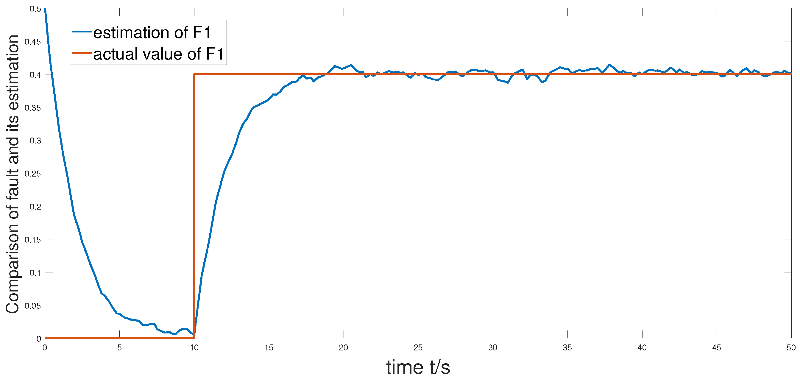
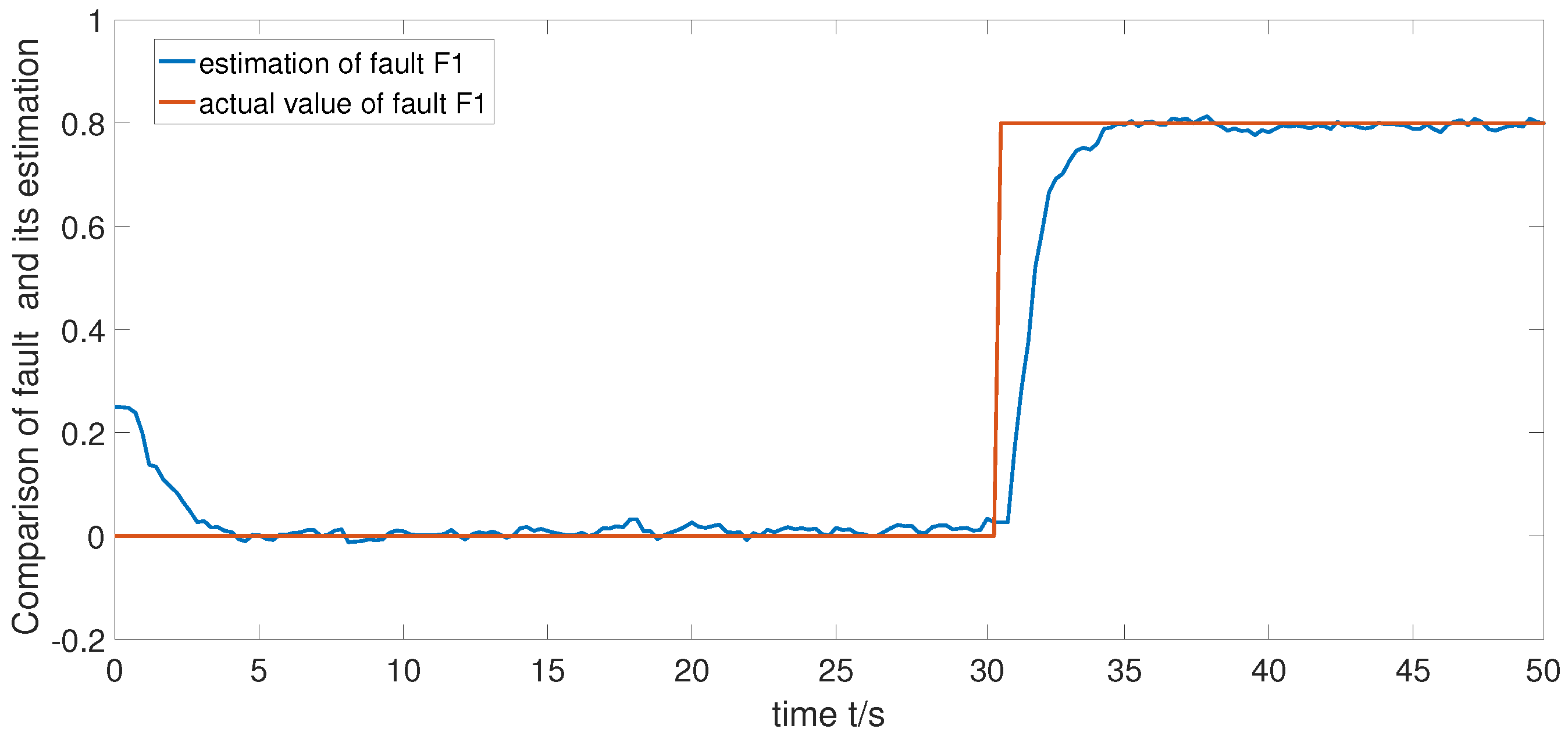
After the fault diagnosis filter is designed based on Theorem 1, we can obtain Figure 5, Figure 6 and Figure 7. Figure 5 is the estimation of F 1 when pickaxe digging occurs. It can be seen from Figure 5 that the fault diagnosis filter can quickly track the change of the fault 10 s after the first destructive vibration source F 1 appears. Figure 6 is the response of the fault diagnosis observer when machine excavation F 2 exists. It can be seen from Figure 6 that, after the second vibration source appears, the fault diagnosis filter can quickly track fault F 2 . Figure 7 is the response of the fault diagnosis observer with multiple faults F 1 (pickaxe digging) and F 2 (machine excavation), which can be detected, respectively, based on the methods in this paper. It can be seen from Figure 7 that, when faults F 1 and F 2 exist at the same time, the diagnostic filter can clearly diagnose F 1 and F 2 . The corresponding vibration source strength can thus be estimated and helps to identify which type of damage.
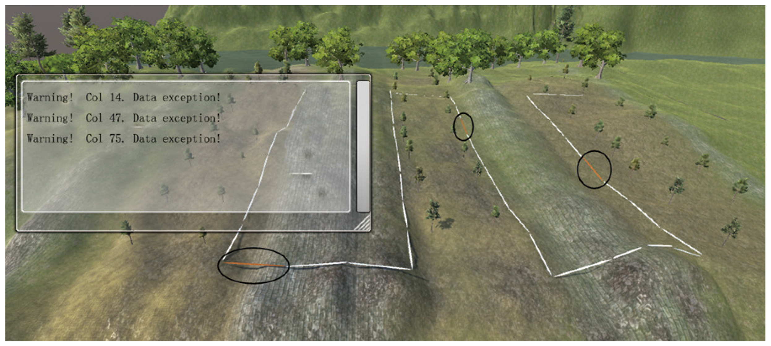
In the man–machine interface designed for the optical fiber vibration source detection and early warning system, we carried out a comparative experiment. We used the same set of data to compare the PDF thresholds. The experiment showed that, before adjusting the threshold value, the detection effect of the optical fiber signal under the influence of vibration is as shown in Figure 8. The platform detects that three columns have vibration alarm signals, and this section flashes to remind the user. The effect after using the method in this paper is shown in Figure 9, which proves that the method of fault isolation can reduce the false alarm rate and make the detection effect of the optical fiber vibration source more stable and accurate.

6. Conclusions

In this paper, in order to reduce the false alarm rate in oil or gas pipeline monitoring, we regarded the different vibrations in the system as faults and considered faults’ isolation to identify different types of vibrations for a non-Gaussian stochastic distribution control model because of inevitable non-stationary interferences from the environment. The fault isolation started by using square root B-spline expansion and a nonlinear weighted dynamic model. The faults in the system were estimated separately to achieve the purpose of fault isolation. The output value of the system in this paper is not measurable, but the output PDFs can be measured by optical instruments. Firstly, the PDFs of the output signal were approximated by square root B-spline expansion. Secondly, the nonlinear dynamic model between the control input and the weights of PDFs was established by a dynamic neural network. Thirdly, based on the measured output PDFs and the input of the system, a filter-based residual generator was constructed to detect and diagnose the faults. Through LMIs, the feasibility criterion for the detection and isolation system faults was given, as well as the steady error ranges. Finally, the effectiveness of this method was verified for the optical fiber vibration source detection system.

7. Future Work

In the optical fiber vibration source detection system, there will be more types of faults, such as time-varying faults, multiplicative faults, etc. This paper only focused on the detection and isolation of constant faults in optical systems. In the future work, we will continue to study the detection and isolation of multiplicative faults and time-varying faults in stochastic distributed systems.

Author Contributions

L.Y., J.L. and T.L. conceived the project. L.Y., J.L. searched relevant literatures. L.Y., J.L. carried out the theoretical derivation. L.Y., J.L., T.L. and H.Q. provided the simulation results. L.Y., J.L. and T.L. analysed the simulation results and wrote the paper. Correspondence and requests for materials should be addressed to L.Y. All authors have read and approved the final manuscript.

Funding

The work in this paper is jointly funded by National Science Foundation of China under Grant Nos. 61573190, 61973168. They are gratefully acknowledged.

Institutional Review Board Statement

Not applicable.

Informed Consent Statement

Not applicable.

Data Availability Statement

Not applicable.

Conflicts of Interest

The authors declare no conflict of interest.

Nomenclature

γ ( z , u ( t ) , F 1 , F 2 ) output PDFs
γ ^ ( z , u ( t ) ) estimated output PDFs
x ( t ) state vector
x ^ ( t ) estimated value of the state vector
F 1 Fault 1
F ^ 1 estimates of fault F 1
F 2 Fault 2
F ^ 2 estimates of fault F 2
v i ( u ( t ) , F 1 , F 2 ) the corresponding weights of B-spline expansion
ω 0 ( z , u ( t ) , F 1 , F 2 ) model error term
b i ( z ) the pre-specified basis functions
y ( t ) system output
e ( t ) state error vector
u ( t ) input of nonlinear stochastic optical fiber vibration detection system
ϵ ( t ) fault detection residual vector
Ppositive definite matrix to be solved
Lgain of fault diagnosis filter
g ( x ( t ) ) nonlinear function
P D F s probability density functions
L M I s linear matrix inequalities
F D I fault detection and isolation

References

  1. Yu, X.; Jiang, B.; Ke, Z. Observer-Based Fault Detection of Broken Rotor Bars in Traction Motors. In Proceedings of the 2017 29th IEEE Chinese Control and Decision Conference (CCDC), Chongqing, China, 28–30 May 2017; pp. 309–314. [Google Scholar]
  2. Venghi, L.E.; Aguilera, F.; de la Barrera, P.M.; De Angelo, C.H. Detection and isolation of current-sensor and open-switch faults in electric traction drives. IEEE Lat. Am. Trans. 2021, 19, 1335–1346. [Google Scholar] [CrossRef]
  3. Qiang, X.; Xue, R.; Zhu, Y. Multi-sensor Fusion Approach with Fault Detection and Isolation Based on two-state Probability Ratio. In Proceedings of the 2021 Sixth International Conference on Wireless Communications, Signal Processing and Networking, Chennai, India, 25–27 March 2021; pp. 325–329. [Google Scholar]
  4. Yin, L.; Wang, H.; Guo, L.; Zhang, H. Data-driven Pareto-DE-based intelligent optimal operational control for stochastic processes. IEEE Trans. Syst. Man Cybern. Syst. 2019, 51, 4443–4452. [Google Scholar] [CrossRef]
  5. Yan, B.; Tian, Z.; Shi, S. A Novel Distributed Approach to Robust Fault Detection and Identification. Int. J. Electr. Power Energy Syst. 2008, 30, 343–360. [Google Scholar] [CrossRef]
  6. Wang, H.; Yao, L.N. Sensor Fault Diagnosis and Fault-Tolerant Control for Non-Gaussian Stochastic Distribution Systems. Math. Probl. Eng. 2019, 50, 1–13. [Google Scholar] [CrossRef] [Green Version]
  7. Yao, L.; Xu, J.; Xu, F. Minimum Entropy Fault-Tolerant Control of the Non-Gaussian Stochastic Distribution System. IET Control Theory Appl. 2016, 10, 1194–1201. [Google Scholar] [CrossRef]
  8. Guo, L.; Wang, H. Fault Detection and Diagnosis for General Stochastic Systems Using B-Spline Expansions and Nonlinear Filters. IEEE Trans. Circuits Syst. I Regul. Pap. 2005, 52, 1644–1652. [Google Scholar]
  9. Cao, S.Y.; Guo, L. Fault Diagnosis with Disturbance Rejection Performance Based on Disturbance Observer. In Proceedings of the 48h IEEE Conference on Decision and Control (CDC) held jointly with 2009 28th Chinese Control Conference, Shanghai, China, 16–18 December 2009; pp. 6947–6951. [Google Scholar]
  10. Zhang, J.; Gao, Q.; Yuan, C.; Zeng, W.; Dai, S.L.; Wang, C. Similar Fault Isolation of Discrete-Time Nonlinear Uncertain Systems: An Adaptive Threshold Based Approach. IEEE Access 2020, 8, 80755–80770. [Google Scholar] [CrossRef]
  11. Wang, H.; Kang, Y.; Yao, L.; Wang, H.; Gao, Z. Fault Diagnosis and Fault Tolerant Control for T–S Fuzzy Stochastic Distribution Systems Subject to Sensor and Actuator Faults. IEEE Trans. Fuzzy Syst. 2021, 29, 3561–3569. [Google Scholar] [CrossRef]
  12. Zhang, Y.W. Data Based Fault Isolation; Northeast University Press: Shenyang, China, 2016. [Google Scholar]
  13. Wang, Y.Q.; Hao, Y.E.; Ding, X.S.; Wang, G.Z. Fault Detection of Networked Control Systems Based on Optimal Robust Fault Detection Filter. Acta Autom. Sin. 2008, 34, 1534–1539. [Google Scholar] [CrossRef]
  14. Yang, L.; Wang, Z.; Xiao, H.; Zhou, D. Least Square Fault Estimation for a Class of Sensor Networks. In Proceedings of the 2013 25th Chinese Control and Decision Conference (CCDC), Guiyang, China, 25–27 May 2013; pp. 4984–4988. [Google Scholar]
  15. Biswas, S.; Nayak, P.K. A Fault Detection and Classification Scheme for Unified Power Flow Controller Compensated Transmission Lines Connecting Wind Farms. IEEE Syst. J. 2021, 15, 297–306. [Google Scholar] [CrossRef]
  16. Tran, M.Q.; Elsisi, M.; Liu, M.K. Effective Feature Selection with Fuzzy Entropy and Similarity Classifier for Chatter Vibration Diagnosis. Measurement 2021, 184, 109962. [Google Scholar] [CrossRef]
  17. Tran, M.Q.; Liu, M.K.; Elsisi, M. Effective Multi-sensor Data Dusion for Chatter Detection in Milling Process. ISA Trans. 2022, 125, 514–527. [Google Scholar] [CrossRef]
  18. Ren, M.F.; Zhang, J.H.; Wang, H. Control and Filtering for Non-Gaussian Systems; Science Press: Beijing, China, 2016. [Google Scholar]
  19. Cheng, Y.; Chen, B.; Zhang, W. Adaptive Multipoint Optimal Minimum Entropy Deconvolution Adjusted and Application to Fault Diagnosis of Rolling Element Bearings. IEEE Sens. J. 2019, 19, 12153–12164. [Google Scholar] [CrossRef]
  20. Guo, L.; Yin, L.; Wang, H.; Chai, T. Entropy Optimization Filtering for Fault Isolation of Nonlinear Non-Gaussian Stochastic Systems. IEEE Trans. Autom. Control 2009, 54, 804–810. [Google Scholar]
  21. Yin, L.; Lai, L.; Zhu, Z.; Li, T. Maximum Power Point Tracking Control for Non-Gaussian Wind Energy Conversion System by Using Survival Information Potential. Entropy 2022, 24, 818. [Google Scholar] [CrossRef]
  22. Shu, M.X. Research on False Alarm Control Algorithm for Fiber Vibration Source Detection under Non-Stationary Disturbances. Master’s Thesis, Nanjing University of Information Science & Technology, Nanjing, China, 2019. [Google Scholar]
  23. Han, D. Alarm Control and Simulation Platform Construction for Disturbed Optical Fiber Vibration Detection. Master’s Thesis, Nanjing University of Information Science & Technology, Nanjing, China, 2020. [Google Scholar]
  24. Cai, Y. Research Progress on Safety State Monitoring Technology of Oil and Gas Pipeline System. Pet. New Energy 2022, 34, 65–70. [Google Scholar]
  25. Wang, H. Bounded Dynamic Stochastic Systems, Modelling and Control; Springer Group: Berlin, Germany, 1999. [Google Scholar]
  26. Guo, L.; Yi, Y.; Yin, L.P.; Wang, H. Modeling, Analysis and Control Theory of Non-Gaussian Stochastic Distribution System; Science Press: Beijing, China, 2019. [Google Scholar]
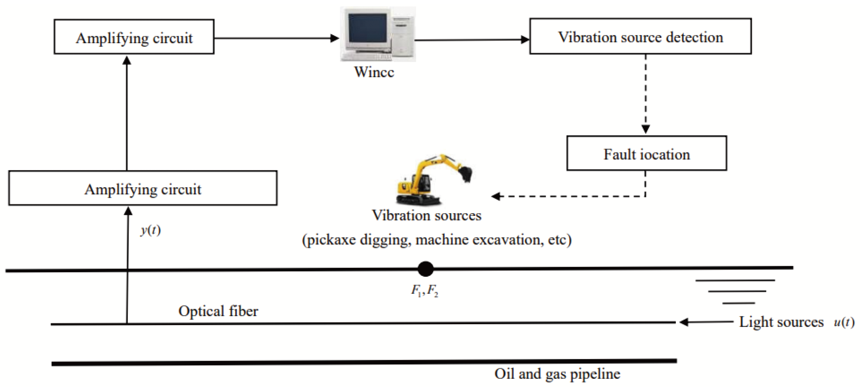
Figure 1. Fiber vibration source detection system.
Mathematics 10 04261 g001
Figure 2. The 3D mesh of output PDFs when F 1 = F 2 = 0 .
Mathematics 10 04261 g002
Figure 3. The 3D measure of output PDFs with faults.
Mathematics 10 04261 g003
Figure 4. Response of residual vector ε ( t ) .
Mathematics 10 04261 g004
Figure 5. Comparison of fault F 1 and its estimation F ^ 1 .
Mathematics 10 04261 g005
Figure 6. Comparison of fault F 2 and its estimation F ^ 2 .
Mathematics 10 04261 g006
Figure 7. Composite graph of F 1 , F 2 , and their estimations F ^ 1 , F ^ 2 .
Mathematics 10 04261 g007
Figure 8. Vibration source alarm before using the isolation method.
Mathematics 10 04261 g008
Figure 9. Vibration source alarm after using the isolation method.
Mathematics 10 04261 g009
Publisher’s Note: MDPI stays neutral with regard to jurisdictional claims in published maps and institutional affiliations.