Reduction in Voltage Harmonics of Parallel Inverters Based on Robust Droop Controller in Islanded Microgrid

Abstract

In this article, a distributed control scheme to compensate for voltage harmonics in islanded microgrids is presented, where each distributed generation (DG) source has a primary control level and a secondary control level. In addition to the voltage and current control loops, the primary control level of DGs includes virtual impedance control loops in the main and harmonic components, which are responsible for dividing the power of the main component and the non-main component (harmonic) between the DGs of the microgrid, respectively. For coordinated operation between the inverters when facing the islanding phenomenon, it is very beneficial to use a droop controller structure. Here, the traditional droop controller is modified in such a way that the power is proportionally divided between the DGs, which causes accurate voltage regulation at the output of the DGs. By presenting a model for the inverter connected to the nonlinear load, a harmonic droop controller is designed. Through the droop controller related to each harmonic, the harmonic voltages are calculated and added to the reference voltage, which improves the quality of the output voltage. Then, the inverter voltage control loop is modified with resistive impedance in the presence of nonlinear loads in such a way that, when combined with the harmonic droop controller, the total harmonic distortion (THD) of the output voltage is significantly reduced. Lastly, the proposed method is implemented on the microgrid through MATLAB software, and the results show the ability of the proposed method to reduce voltage harmonics in the parallel operation of inverters.

1. Introduction

Challenges such as increasing energy demand, wear and tear of network equipment, harmful effects on the environment, increasing energy prices, and increasing dependence of countries on energy imports are among the main motivations for moving toward achieving stable, safe, and competitive energies with existing energy sources [1,2]. For this reason, specialists are planning to increase the efficiency, power quality, and reliability of the electric energy distribution system by developing current networks and moving toward smart networks [3,4,5]. Microgrids are among the controllable and constructive components of a smart distribution network. A microgrid is a local network that consists of distributed generation, energy storage systems, and local loads. These devices are designed in such a way that they can continue to feed local loads in two modes of connection to the grid or island from it [6,7,8]. To guarantee the reliable operation of a microgrid in an island mode, it is necessary to divide the power demand between the resources in a predetermined ratio, regardless of the network parameters. To divide the power of DGs in an independent AC system, in conditions where there is no telecommunication connection between them, the conventional droop method is used. This method is an example of the technique used to divide power between synchronous generators in a large power system [9,10,11,12].

DGs are often connected to microgrids through electric power interface converters, where the main role of an interface converter is to control the injection power. One of the problems of using this type of converter in DG is creating harmonics in the network [13,14,15]. The inverter type of DGs has a greater effect on the power quality issues of the network, such as the generation of harmonics injected into the network [16,17,18]. The increasing growth of devices sensitive to power quality and the use of DGs based on inverters are among the most important reasons for there having been extensive focus on the concept of microgrid power quality during the past decade [19,20,21]. Therefore, it is necessary to identify the types of harmonics and the best methods to remove them so as to reduce them to a permissible level.

Power quality problems and voltage harmonics can be improved by applying appropriate strategies. One of these methods is the use of virtual impedance in the DG control system for harmonic frequencies to compensate for the harmonic components of the voltage [22,23,24]. A unified power quality conditioner (UPQC) acts as an active filter to compensate for load current harmonics and voltage fluctuations in both island mode and network connection. UPQC is capable of compensating for undervoltage, overvoltage, and harmonics of voltage and current using parallel and series inverters [25,26,27]. In the parallel operation of inverter-based DGs, control operations in the frequency domain are used to solve power quality problems such as harmonics and disturbances, which can be implemented via local control of each inverter-based DG. Power sharing and voltage regulation are centrally controlled, and commands are sent through a telecommunication link with low bandwidth. In this method, the inherent quick response of inverters is used, and the waveform quality functions in high bandwidth controllers are sent to each local inverter. Therefore, the voltage balance under severe load imbalances is guaranteed, and the voltage quality is also improved [28,29]. By injecting reactive power using a static distribution compensator in microgrid islanding mode, the required voltage stability under voltage drop is provided; as a result, the microgrid power quality is improved [30,31,32].

DGs connected to the network have two types of current or voltage control loops. While most of the research has been conducted to reduce harmonics on DGs with the current loop control, the process of improving power quality control through the voltage loop has more flexibility than the power quality control using the current loop [33,34]. To increase the voltage quality of DGs when connected to the network, methods have been provided to selectively remove a specific harmonic; thus, the quality of the point common coupling (PCC) voltage is increased by appropriately controlling the DGs connected to the network [35,36]. Using a hierarchical control scheme, it is possible to improve the output voltage quality of DGs connected to sensitive nonlinear loads in a microgrid. This structure includes the primary level and the secondary level of control in the microgrid. In the primary level of control, using a virtual impedance control loop, the fundamental and harmonic components of the load are divided between DGs. This type of load sharing may cause an increase in harmonic disturbances. On the other hand, the secondary level of control sends an appropriate signal to the primary level of control to compensate for voltage unbalance and harmonics and improve the power quality [37,38].

In [39,40], a method to control power and eliminate harmonics in inverter-based DGs with a current control loop was presented. In this method, due to the independent operation of two parallel controllers, the current of the fundamental component and the harmonic component without the need for the feedback of the load current and the voltage of the connection to the network, power control, and the removal of harmonics were established. Using a variable reactor based on magnetic flux, the integrated power quality controller (IPQC) was designed in such a way that the microgrid power quality problems such as harmonics and voltage fluctuations can be solved. For the fundamental component, the impedance is equivalent to the impedance of the variable reactor, and, for the harmonic component of the n-th order, the impedance is very high and acts as a filter [41,42].

By modifying the conventional droop controller, a harmonic droop controller is designed. The amount of voltage that should be added to the harmonic components of the reference voltage is calculated as a function of the characteristics of voltage and frequency droop control, and then added to the value of the reference voltage of the fundamental component. In this way, the THD of the output voltage is reduced [43]. One of the problems of using the frequency and voltage droop strategy is the presence of nonlinear loads in the system. To solve this problem and increase the output voltage quality of inverter-based DGs, linear and nonlinear loads are first proportionally divided between DGs. The absolute of the current corresponding to the harmonic component is measured and the voltage drop corresponding to its h-th harmonic component is calculated. Then, to reduce the harmonic component, a signal whose amplitude is proportional to the droop coefficient and whose phase is the opposite of the harmonic component is added to the reference voltage, thus improving the THD of the output voltage [44].

Literature Review

Parallel inverters with LCL output filters have small inertia and effectively form a weak network. Any harmonic current that spreads in this network causes voltage distortion at the point of common connection (PCC). This harmonic voltage may challenge the stability of the microgrid due to the existing resonance. In addition, according to the existing standards, the THD of the microgrid voltage should be less than 2.5%. Therefore, the harmonic damping should be such that the microgrid works according to these standards. Conventional techniques include installing active and passive filters to balance harmonics. These methods may cause resonance and network stability problems. Therefore, the inverter control strategy can be used to improve power quality. In [45], it was proposed to produce a sinusoidal voltage at the PCC point with non-sinusoidal inverter operation and pulse width modulation control. The proposed algorithm corrects voltage harmonics in the PCC. In recent years, extensive research has been presented in the field of microgrid harmonic control based on the virtual impedance algorithm [46,47].

In [48], current harmonic control in an islanded microgrid based on stability analysis was presented. The proposed model based on the proportional droop method showed the harmonic compensation of current caused by mismatch and proportional distribution of power. In [49], the harmonic current control model based on eliminating the output impedance mismatch of DG units based on the virtual impedance method was presented. In [50], the voltage harmonic compensator model at the AC microgrid connection point to the main grid based on the virtual impedance method was presented. Nevertheless, one of the most important challenges of using the virtual impedance theory is the precise determination of the virtual impedance factor to increase the accuracy of the control method. In [51], a small signal analysis model and, in [52], a Lyapunov control method for determining the optimal and practical range of virtual impedance were presented. Although this method was effective in determining the droop coefficients and virtual impedance, the droop stability was highly dependent on the designed droop coefficients and virtual impedance.

In this article, firstly, the limitations of the conventional droop method are investigated. It is determined that, to accurately share power between DGs in parallel operation, the per-unit values of the coupling impedance, as well as the effective value of the output voltage of the DGs, must be equal. However, in practice, due to the existence of computational errors, disturbance and noise cannot establish such conditions. To reduce the limitations and accurate power sharing between parallel DGs in the island mode, the conventional droop controller is modified. The presented strategy shows good performance in two modes, islanded and connected to the network. In this method, the accuracy of load sharing does not depend on the coupling impedance and the voltage value of inverter-based DGs. The proposed method is also robust against disturbances, noise, and computational errors. The proposed controller compensates for the voltage drop caused by the load increase and the droop characteristics, as well as improves the voltage regulation. A new method for reducing the harmonic components of the DG output voltage is presented using the droop strategy. In this method, the amount of voltage that needs to be added to the harmonic components of the reference voltage to reduce the harmonic power of the DG output voltage is calculated through the characteristics of the harmonic droop control; thus, the harmonic components of the output voltage, as well as its THD, are reduced to some extent. Due to the limitation in the selection of harmonic droop coefficients, when feeding sensitive loads, the harmonic droop controller alone is not able to reduce the voltage harmonics to the permissible limit. Therefore, by providing a voltage control loop, the inverter-based DG is modeled as a source with a predominantly resistive coupling impedance. By modifying this control loop and combining it with the harmonic droop controller, the quality of the output voltage is significantly improved. The simulation results show that the proposed method can accurately share active and reactive power in the parallel operation of inverters in the presence of nonlinear loads, improve voltage regulation, and reduce voltage THD. The remainder of the article is structured as follows: in Section 2, the general control structure of the microgrid is described; in Section 3, the proposed control method is introduced; in Section 4, the simulation results are presented; lastly, in Section 5, the conclusion is presented.

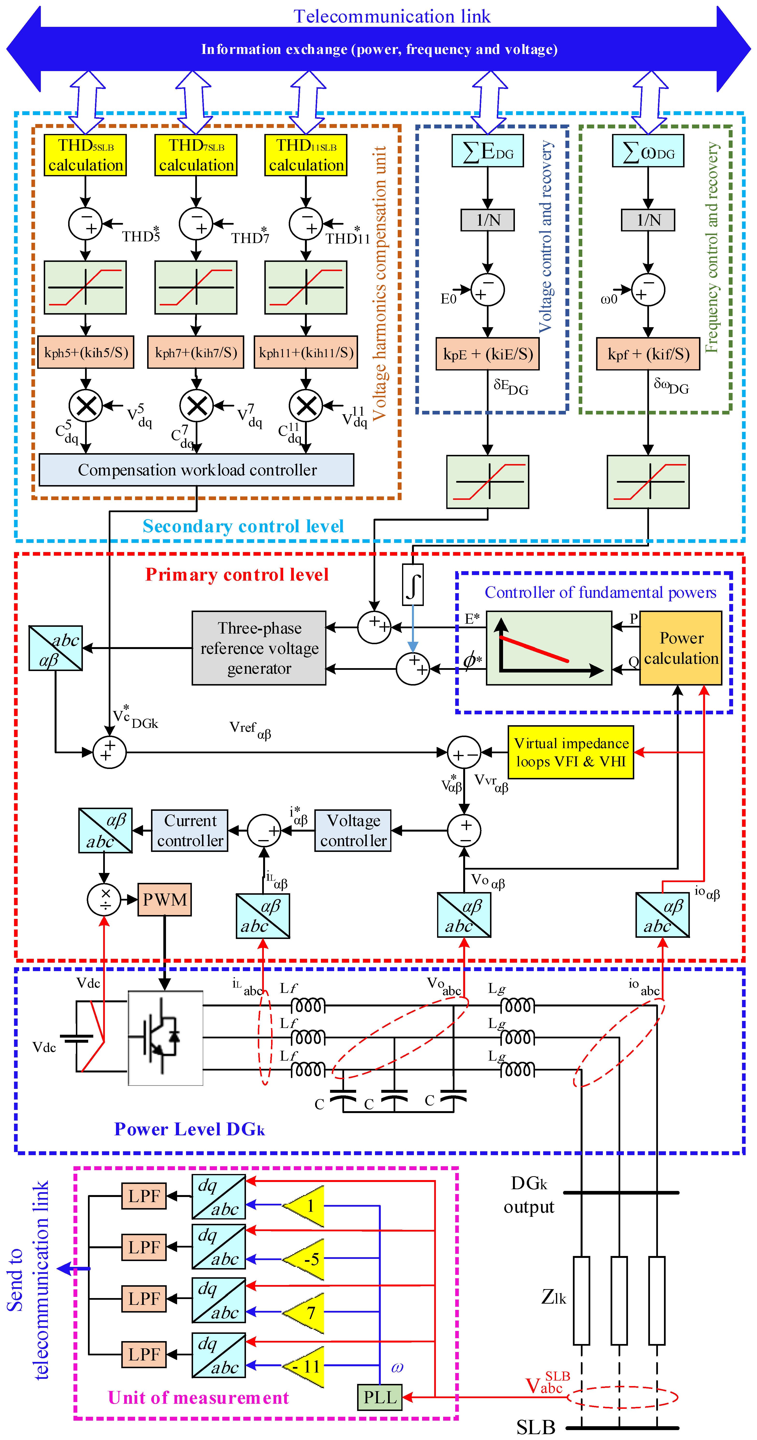
2. Microgrid Control Infrastructure Based on a Primary and Secondary Control

Figure 1 shows the general structure of the control method and how to implement it in an island microgrid. This microgrid includes some DGs that are connected to the “source bus” by electronic power converters and distribution lines. Each DG may consist of a power generator and energy storage system. Furthermore, some linear and nonlinear loads are connected to the sensitive load bus (SLB) of the microgrid. The structure of the power section and the details of the primary and secondary control levels of each DG are presented in Figure 2. The power section of each DG includes a DC link, an interface inverter, and an LCL filter. It is worth mentioning that the focus of this article is on DG interface inverter control. Therefore, it is assumed that an almost constant DC voltage (v_dc) is always provided in the DC link. However, as can be seen in Figure 2, to consider the potential fluctuations of the DC link voltage, a feed-forward loop is used in the generation of inverter gate signals by the pulse width modulator (PWM) block.

As shown in Figure 1, each DG has two primary and secondary control levels, both of which are implemented locally and side by side. In this method, there is no communication between the primary and secondary control levels, and the secondary controllers apply the necessary control signals to the primary controllers based on the measurements taken from the output of DGs and SLB. According to Figure 2, the primary control level of DGs includes power control droop characteristics, voltage and current control loops, and virtual impedance loops.

The control at the secondary level is performed in a distributed way, and the necessary references are sent to the primary controllers to regulate the output voltage and fundamental frequency of DGs, as well as compensate for the harmonic disturbances of the SLB voltage. Since the distance between the load bus and the source bus may be large, the load bus voltage information is sent to the secondary controllers using a low bandwidth communication (LBC) link. The choice of LBC was made to avoid the dependence of the control system performance on the presence of high bandwidth (which can reduce the reliability of the system). On the other hand, to have sufficient low bandwidth, the data transmitted by LBC should include approximately DC signals. Therefore, the main and harmonic components of the SLB voltage are first extracted in the synchronous reference frame (dq) and then sent to the secondary controller DGs. Note that, in this article, the fifth-, seventh-, and 11th-order harmonics are compensated for as the main harmonics. The details of the separation of the main and harmonic components of the SLB voltage are shown in the “measurement block” of Figure 2.

2.1. Primary Control Level of DGs

The DG control system is designed in the stationary reference frame (αβ), within which the conventional Clark transformation relations are used to transfer variables between the abc and αβ frames. As shown in the primary control block DG_k in Figure 2, the DG output voltage reference in the frame (v*_αβ) is generated by the droop characteristics, virtual impedance loops, and SLB voltage harmonics compensation reference (v*_c). On the other hand, the instantaneous voltage of the output filter of the inverter (v_Oabc) is transferred to the reference frame αβ; then, after comparing with v*_αβ, it provides the current control reference i*_αβ. Lastly, the response of the current controller is returned to the abc frame according to the error resulting from the comparison of the output inductor current of the filter and the reference current i*_αβ. Hence, the three-phase reference voltages are generated to be applied to the PWM block, and the inverter is switched on the basis of this reference. Note that, in the design of virtual impedance loops, to properly apply the droop characteristics in controlling the power of the main component, the parameters of the harmonic virtual impedance loops should be determined in such a way that the microgrid has mainly inductance/impedance. Furthermore, a small virtual resistance can help to dampen system fluctuations.

The details of the implementation of the secondary controller of each of the DGs are presented in Figure 2, where the secondary controller of each DG consists of voltage recovery, fundamental frequency recovery, and SLB voltage harmonic compensation units.

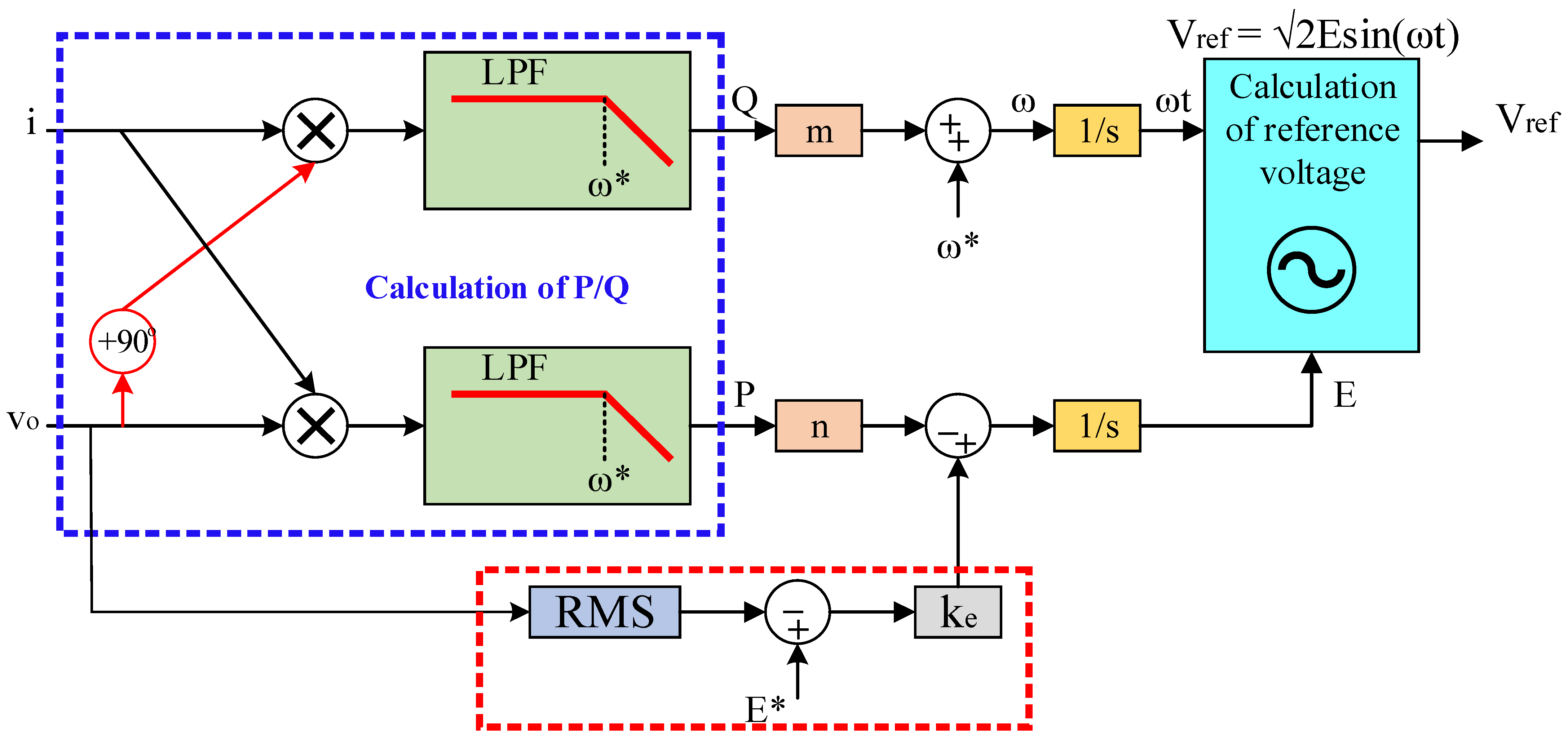
2.2. Fundamental Frequency Control

As seen in Figure 2, at each sampling time, the DG_k output fundamental frequency is compared with the average output frequency of all units, and the resulting error is used to recover the DG_k frequency. The fundamental frequency recovery signal for each DG can be expressed using Equation (1).

$$\begin{array}{c}\delta {\omega }_{D{G}_k}=k_{pf}\left({\omega }_0-{\overline{\omega }}_{D{G}_k}\right)+k_{if}{{\displaystyle \int }}^{ }\left({\omega }_0-{\overline{\omega }}_{D{G}_k}\right)dt\\ {\overline{\omega }}_{D{G}_k}=\frac{{{\displaystyle \sum }}_{i=1}^N{\omega }_{D{G}_k}}{N}\end{array},$$

(1)

where ${\overline{\omega }}_{D{G}_k}$ is the average value of the measured frequencies, ω₀ is the reference frequency, and $\delta {\omega }_{D{G}_k}$ is the control signal that is calculated by the secondary controller to control and recover the output fundamental frequency of DG_k at each sampling time. Here, N is the number of frequencies sent to the telecommunication system after sampling. To analyze and determine the characteristic parameters of P–ω droop and the secondary frequency controller, the block diagram of the small signal model of the secondary controller of frequency for DG_k is shown in Figure 3. As can be seen, microgrid fundamental frequency control is achieved by secondary controllers and P–ω droop controllers. In Figure 3, the G_LPF block is a low-pass filter for power calculation, the G_PLL block is a first-order transfer function for DG frequency extraction, the G_fsec block is a PI controller, and ka is the proportional gain.

A low-pass filter (G_LPF(s)) is considered in the modeling of droop controllers to calculate the power of the main component. Furthermore, secondary control modeling by a simple phase-locked loop (PLL) with the first-order transformation function G_PLL(s) is used to estimate the DG output fundamental frequency and a proportional coefficient (k_a) to determine the average value of the frequency (Δω_avg) as a function of the measured frequencies and a PI controller with the G_fsec(s) transformation function. The characteristic equation of the block diagram presented in Figure 3 can be expressed as Equation (2).

$$\begin{array}{c}\Delta f=1+G_{LPF}\left(s\right)·G_P\left(s\right)·\frac{1}{s}·G+G_{PLL}\left(s\right)·k_a·G_{f_{sec}}\left(s\right)\\ G=\frac{V_{k0}{V}_{PCC}\cos \left({\phi }_{k0}-{\phi }_{PCC}\right)}{X_k}\end{array}.$$

(2)

In Equation (2), V_k0 and φ_k0 are reference voltage and angle DG_k, respectively, V_PCC is the voltage at the PCC point, φ_PCC is the angle difference between DG_k and the PCC point, X_k is the inductance between the PCC point and DG_k, and k_a = 1/N is a coefficient that determines the average value of the fundamental frequency. The transformation function of other parts of the small signal model of the frequency controller is as follows:

$$\begin{array}{c}{G}_{LPF}\left(s\right)=\frac{1}{1+{\tau }_{p}s}\\ G_{PLL}\left(s\right)=\frac{1}{1+\tau s}\\ G_{f_{sec}}\left(s\right)=\frac{k_{pf}s+k_{if}}{s}\end{array}.$$

(3)

By analyzing the eigenvalues obtained from Equation (2), it is possible to correctly adjust the parameters of the P–ω droop characteristic and the secondary controller in DG_k to achieve the minimum amount of frequency deviation.

2.3. Voltage Control

As in the previous section, a similar method can be used for distributed voltage control based on the deviation of the average voltage of all DGs from the nominal value. The advantage of this method compared to the central secondary control method is that, in the distributed control method, the need to measure information from a distance is eliminated. According to Figure 2, at each sampling time, the effective value of the output voltage of each DG is sent to all other DGs to determine the average effective voltage of the microgrid (${\overline{E}}_{D{G}_k}$), and, after comparing it with the nominal voltage value ($E_0$), the control signal and voltage recovery ($\delta E_{D{G}_k}$) are produced locally by the secondary controller DG_k. In this case, the DG_k voltage distributed controller can be implemented at the secondary level by Equation (4).

$$\begin{array}{c}\delta E_{D{G}_k}=k_{pE}\left(E_0-{\overline{E}}_{D{G}_k}\right)+k_{iE}{{\displaystyle \int }}^{ }\left(E_0-{\overline{E}}_{D{G}_k}\right)dt\\ {\overline{E}}_{D{G}_k}=\frac{{{\displaystyle \sum }}_{i=1}^N{E}_{D{G}_k}}{N}\end{array}.$$

(4)

In Equation (4), k_pE and k_iE are the proportional and integral coefficients of the PI controller for DG voltage control, respectively. Similar to the previous section, here we can derive the small signal model of the distributed secondary controller for voltage control based on Equation (4). The block diagram of the small signal model of the distributed secondary controller for voltage recovery is presented in Figure 4. On this basis, the characteristic equation of the small signal block diagram model of distributed voltage control can be expressed as shown in Equation (5).

$$\Delta E=1+\left(G_{LPF}\left(s\right)·H·G_Q\left(s\right)\right)+\left(k_a·G_{E_{sec}}\left(s\right)\right),$$

(5)

where the transformation function of different parts is as follows:

$$\begin{array}{c}{G}_Q\left(s\right)=k_{pQ}\\ G_{E_{sec}}\left(s\right)=\frac{k_{pE}s+k_{iE}}{s}\end{array}.$$

(6)

Here, G_Esec(s) is the transformation function of the voltage PI controller at the secondary level, and k_pQ is the proportional coefficient of the reactive power control. As can be seen in Equation (4), the integral coefficient is not considered to control the voltage amplitude. The use of this coefficient is not allowed in the conditions where the microgrid is in island mode, because, in island mode, if integral coefficients are used in the Q–E characteristics, the power injected by DGs does not match the load of the microgrid, and this factor can cause system instability. By analyzing the eigenvalues obtained from Equation (5), it is possible to correctly adjust the parameters of the Q–E reduction characteristic and the secondary controller in DG_k to achieve the minimum voltage deviation.

2.4. Compensation of Microgrid Voltage Harmonics

The operation of the voltage harmonics compensator is different from the operation of the voltage and fundamental frequency control units. Because the voltage and frequency control of the microgrid is based on the average output voltage and frequency of all DGs, the compensation of harmonics should be performed on the basis of the parameters sampled from the SLB. If the goal is to improve the output power quality of DGs, it will be possible to use a structure similar to the voltage and frequency control units at the secondary level. As shown in Figure 2, the main and harmonic components of the SLB voltage are separated in the measuring block and sent to the telecommunication link. Then, in the voltage harmonic compensator block, a harmonic disturbance index (THD^h_SLB) is calculated according to Equation (7) for each of the fifth-, seventh-, and 11th-order harmonics. Here, THD⁵_SLB, THD⁷_SLB, and THD¹¹_SLB are compared with reference values THD*₅, THD*₇, and THD*₁₁, respectively, and errors are given to PI controllers. The output of these controllers is multiplied by v⁵_dq, v⁷_dq, and v¹¹_dq, respectively, to calculate C⁵_dq, C⁷_dq, and C¹¹_dq. If any of the harmonic disturbance indices is less than the reference value, the corresponding saturation block prevents the increase in the disturbance by the PI controller.

$$TH{D}_{SLB}^h=\frac{\sqrt{{\left(v_d^h\right)}^2+{\left(v_q^h\right)}^2}}{\sqrt{{\left(v_d^1\right)}^2+{\left(v_q^1\right)}^2}}\times 100.$$

(7)

In Figure 2, the compensation workload control block adjusts the effort of each DG to compensate for harmonics. The structure of this controller is shown in Figure 5, where S₀, S_fr, and S_r are the “nominal capacity of DG”, “its free capacity to provide non-main component power”, and “remaining capacity after providing non-main component power”, respectively. The details of the S_fr calculation based on the nominal capacity and power value of the main component are shown in Figure 5. In this figure, S_f and S_n are the apparent powers of the main and non-main components, respectively. In addition, the total power supplied by each DG can be calculated as shown in Equation (8).

$$S=\sqrt{{\left(S_f\right)}^2+{\left(S_n\right)}^2}.$$

(8)

Therefore, the performance of the “droop characteristic” block in Figure 5 can be expressed as shown in Equation (9).

$$C_{dq,k}^h=\{\begin{array}{cc}{C}_{dq}^h·\left(S_{fr}-S_n\right)& S_r>0\\ 0& S_r\le 0\end{array}.$$

(9)

According to Equation (9), if S_r > 0 (not exceeding the rated capacity of DG), C^h_dq,k decreases with increasing S_n (increasing effort of DG for compensation), which means reducing the effort of DG_k for compensation. In other words, in this method, there is inherent feedback that leads to the proper division of workload between DGs. In the end, after multiplying the harmonic compensation reference h (C^h_dq) by S_r, the compensation signal of this harmonic (C^h_dq,k) is calculated for DG_k, and, by adding the main harmonics compensation references in the static reference frame, the total compensation reference of SLB voltage harmonics (v*_c) is produced.

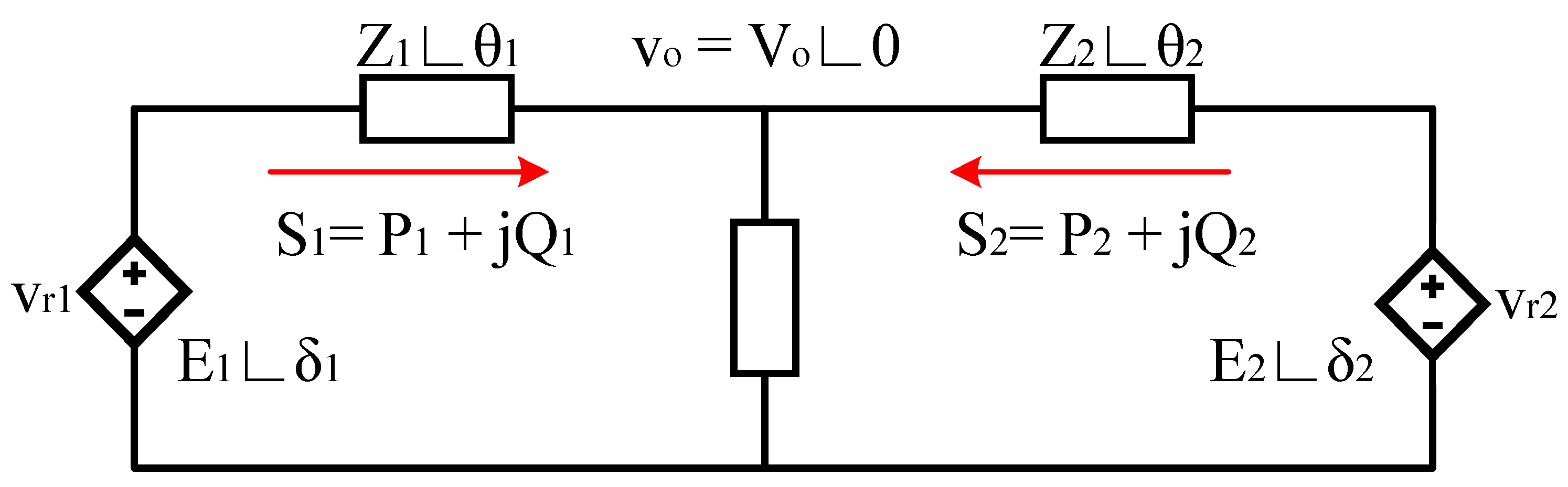
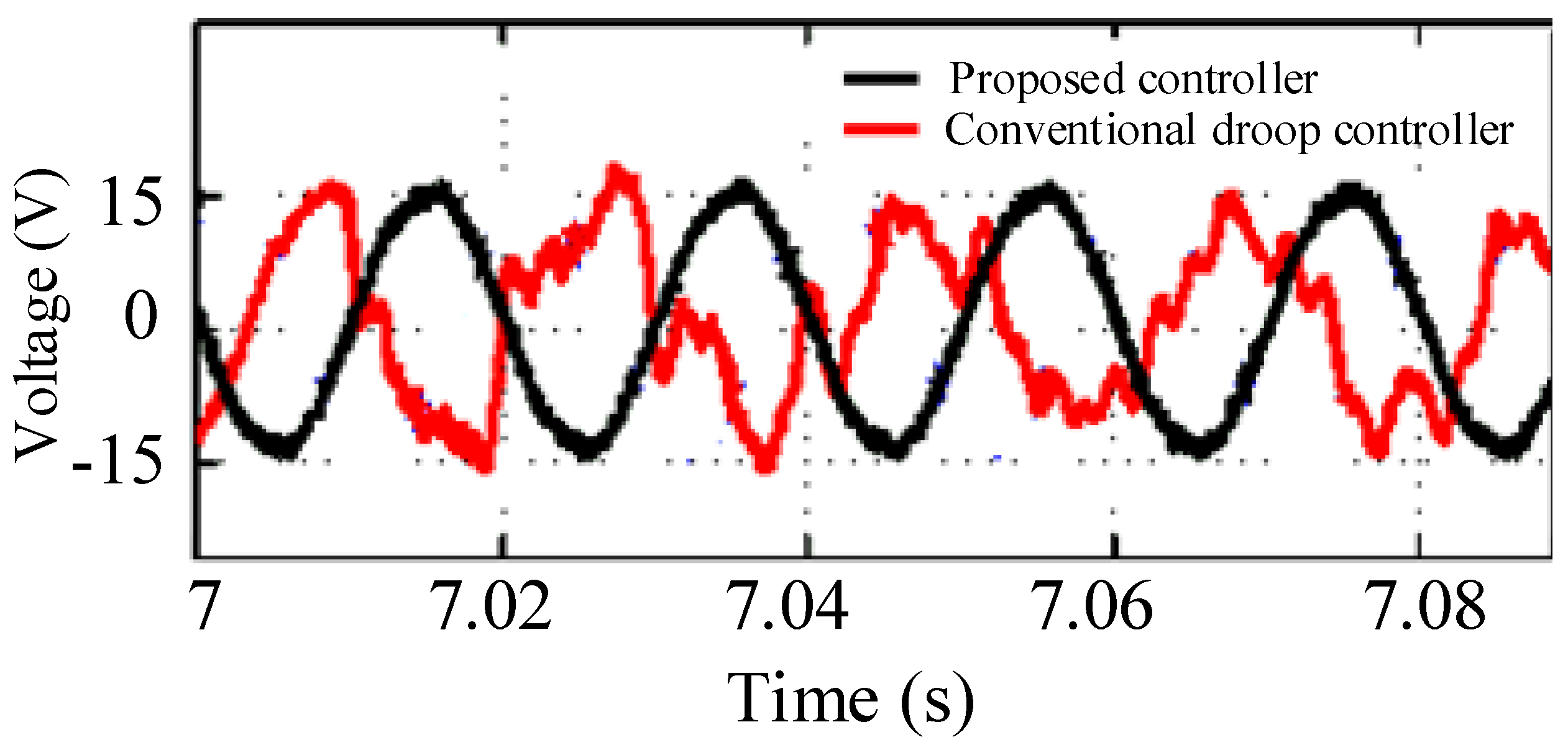
3. The Structure of the Proposed Controller Based on the Modification of the Conventional Droop Controller

The proper performance of the microgrid in both grid-connected and island mode requires efficient power control and voltage regulation methods. Preferably, in these methods, telecommunication links should not be used between sources that are located at far distances from each other. Therefore, the control algorithm in each of the distributed generation sources should only use locally measured variables. For this purpose, the conventional droop control is generally used to operate the microgrid in island mode. To investigate the limitations of the droop controller in power sharing, two inverters with output impedance Z₁ and Z₂, which have a parallel operation are shown in Figure 6. The output impedance of the inverters is designed in such a way that the impedance of the line against it can be ignored. The reference voltage of inverters is expressed in Equations (10) and (11).

$$v_{r1}=\sqrt{2}{E}_{1}sin\left({\omega }_{1}t+{\delta }_1\right),$$

(10)

$$v_{r2}=\sqrt{2}{E}_{2}sin\left({\omega }_{2}t+{\delta }_2\right),$$

(11)

where E₁ and E₂ is the effective value of the source voltage. The load voltage is also calculated from Equation (12).

$$v_o=v_{r1}-R_{o1}{i}_1=v_{r2}-R_{o2}{i}_2.$$

(12)

According to Equation (12), the output voltage decreases with increasing load, causing weak voltage regulation in the inverter-based DG output. According to Figure 6, the active and reactive power that each inverter injects into the load is calculated using Equations (13) and (14).

$$P_i=\frac{E_i{V}_o\cos {\delta }_i-V_o^2}{R_{oi}}.$$

(13)

$$Q_i=\frac{-E{V}_o}{R_o}\sin {\delta }_i.$$

(14)

As a result, the voltage and fundamental frequency droop characteristics for the case where the coupling impedance is predominantly resistive (Z₁ = R_o1 and Z₂ = R_o2) are obtained from Equations (15) and (16). Figure 7 shows the conventional droop controller.

$$E_i=E^{\ast }-n_i{P}_i,$$

(15)

$${\omega }_i={\omega }^{\ast }-m_i{Q}_i,$$

(16)

where E* and ω* are the effective value of voltage and angular frequency, respectively, in no-load mode. The selection of droop coefficients n_i and m_i are based on the nominal capacity of the sources (P* and Q*) and the maximum acceptable changes for the frequency and voltage of the source.

To share the load between the units in proportion to the capacity of the generation units, the slope values of the characteristics must be established according to Equations (17) and (18).

$$n_1{s}_1^{\ast }=n_2{s}_2^{\ast }.$$

(17)

$$m_1{s}_1^{\ast }=m_2{s}_2^{\ast }.$$

(18)

Equation (19) can be concluded from the above equations.

$$\frac{n_1}{m_1}=\frac{n_2}{m_2}.$$

(19)

By replacing Equation (15) in Equation (13), the active power is calculated from Equation (20).

$$P_i=\frac{E^{\ast }\cos {\delta }_i-V_o}{n_i\cos {\delta }_i+\frac{R_{oi}}{V_o}}.$$

(20)

By replacing Equation (20) in Equation (15), the difference in the voltage amplitude of two inverter-based DGs is calculated from Equation (21).

$$\Delta E=E_1-E_2=\frac{E^{\ast }\cos {\delta }_1-V_o}{\cos {\delta }_1+\frac{R_{o1}}{n_1{V}_o}}-\frac{E^{\ast }\cos {\delta }_2-V_o}{\cos {\delta }_2+\frac{R_{o2}}{n_2{V}_o}}.$$

(21)

The voltage difference between two inverter-based DGs leads to improper power sharing between DGs. For the voltage droop characteristic to lead to proper active power sharing between DGs in proportion to their rated capacity, Equation (22) must be established.

$$n_1{P}_1=n_2{P}_2.$$

(22)

The voltage difference ΔE according to Equation (15) should be equal to zero. It is very difficult to establish such conditions due to the existence of calculation errors, disturbance, and deviation of parameters. According to Equation (21), this state is realized if Equations (23) and (24) hold.

$$\frac{n_1}{R_{o1}}=\frac{n_2}{R_{o2}}.$$

(23)

$${\delta }_1={\delta }_2.$$

(24)

In other words, n_i should be chosen according to the coupling impedance R_oi of inverter-based DG. As a result, according to Equation (17), the coupling impedance of the inverter-based DG should be selected in such a way that it applies to Equation (25).

$$R_{o1}{s}_1^{\ast }=R_{o2}{s}_2^{\ast }.$$

(25)

The coupling impedance per-unit value of the i-th inverter-based DG is obtained from Equation (26).

$${\gamma }_i=\frac{R_{oi}}{\frac{E^{\ast }}{I_i^{\ast }}}=\frac{R_{oi}{s}_i^{\ast }}{{\left(E^{\ast }\right)}^2}.$$

(26)

As a result,

$${\gamma }_1={\gamma }_2.$$

(27)

This means that, during the parallel operation of the inverter-based DGs to accurately share the active power between the DGs in proportion to their capacity, when the conventional droop strategy is used, the values of the coupling impedance of the inverter-based DGs must be the same. The frequency droop method usually leads to precise sharing of reactive power between DGs in proportion to their capacity in a stable system, because the frequency is a universal signal in the system, and the reactive power of inverter-based DGs is also very sensitive to frequency changes. As a result,

$$m_1{Q}_1=m_2{Q}_2.$$

(28)

Therefore, according to the droop coefficients, m_i in Equations (18) and (29) is valid.

$$\frac{Q_1}{s_1^{\ast }}=\frac{Q_2}{s_2^{\ast }}.$$

(29)

According to Equation (14),

$$m_1\frac{E_1{V}_o}{R_{o1}}\sin {\delta }_1=m_2\frac{E_2{V}_o}{R_{o2}}\sin {\delta }_2.$$

(30)

If δ₁ = δ₂ and E₁ = E₂, then m₁/R_o1 = m₂/R_o2. As a result,

$$C_1:\{\begin{array}{c}{E}_1=E_2\\ \frac{n_1}{R_{o1}}=\frac{n_2}{R_{o2}}\end{array}\leftrightarrow C_2:\{\begin{array}{c}{\delta }_1={\delta }_2\\ \frac{m_1}{R_{o1}}=\frac{m_2}{R_{o2}}\end{array}.$$

(31)

Equation (31) states that, if the inverter-based DGs with resistance coupling impedance divide the active power between the DGs under C₁ conditions, the reactive power is also proportionally divided between the DGs. Furthermore, if the same DGs divide the reactive power between DGs under C₂ conditions, the active power is proportionally distributed between DGs. During the parallel operation of inverter-based DGs, to accurately divide the active power between DGs according to their capacity, when the conventional droop strategy is used, the impedance per-unit values of inverter-based DGs should be the same, and the voltage difference between two DGs should be zero. However, in practice, it is not possible to establish such conditions due to the existence of calculation errors, disturbance, and noise; in fact, establishing these conditions is a sufficient and not a necessary condition for the accurate sharing of power between DGs.

Figure 8 shows the control block diagram of the proposed method. As can be seen, by multiplying the measured output current of the DG by the value calculated for the virtual impedance, the value of the virtual voltage drop is obtained. If the DGs in the microgrid work at the same point of work, active and reactive power sharing is achieved ideally between the DGs. By properly setting the virtual impedance for each unit, the output impedance difference of the DGs can be adjusted, but the common and local loads, as well as the X/R ratio of the network, may change. Therefore, it is necessary to update the designed value for the virtual impedance with the changes made in the system.

To solve the above problems and adjust the voltage properly, it is necessary to enter feedback in the control circuit according to the control principles of the voltage drop of the E* − V_o DG. The (E* − V_o) error signal makes the desired control command by using a proportional controller with gain factor k_e. By adding the control command to ΔE, the voltage drop on the resistance is partially compensated for and the output voltage is within the allowed range. This strategy significantly reduces the effects of calculation errors, disturbances, and noise. According to Figure 8, in a stable system, the input value of the integrator block is zero; as a result, Equation (32) holds.

$$n_i{P}_i=k_e\left(E^{\ast }-V_o\right).$$

(32)

The right side of Equation (32) is the same for all inverter-based DGs that work in parallel and have the same proportional gain k_e; therefore, n_iP_i is equal to a constant value. As a result, this strategy leads to accurate power sharing between DGs and proper voltage regulation at the output of the inverter, and the accuracy of power sharing is not affected by the system parameters.

Therefore, the advantages of the Figure 8 controller can be expressed as follows:

• In conventional droop control methods, to accurately share the load between parallel inverters, the inverters must have the same resistive impedances and voltage setpoints, which, in this method, do not need to meet these two conditions.
• With this strategy, the voltage drop caused by the load can be compensated for, and the voltage can be maintained within a certain range.
• The proposed method can be used for mainly inductance/impedance inverters by applying the Q–E and P–ω droop characteristics.
• In the proposed method, the effects of calculation errors, disturbances, and noise are significantly reduced, and the accuracy of power sharing is not affected by the system parameters.

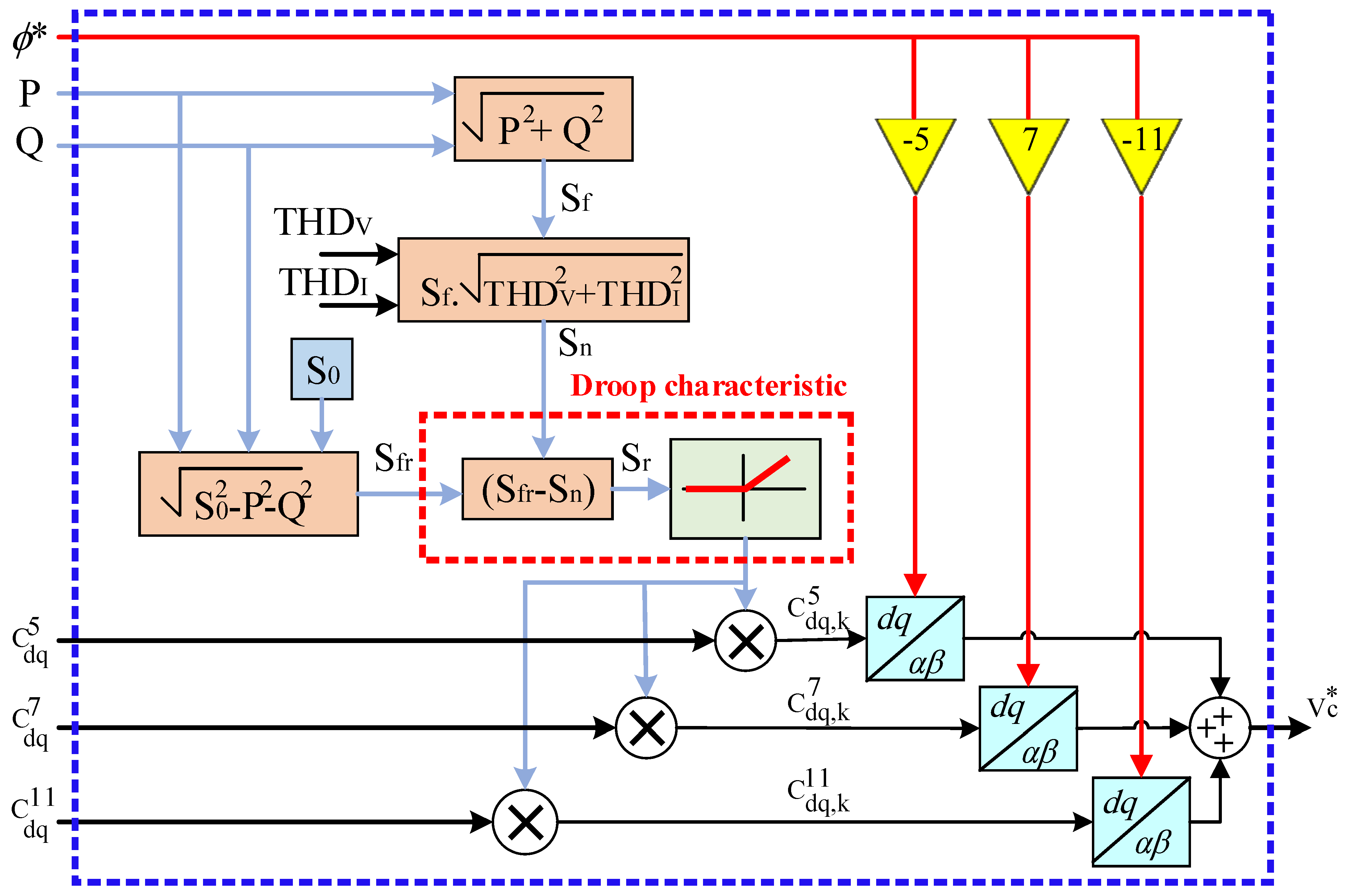
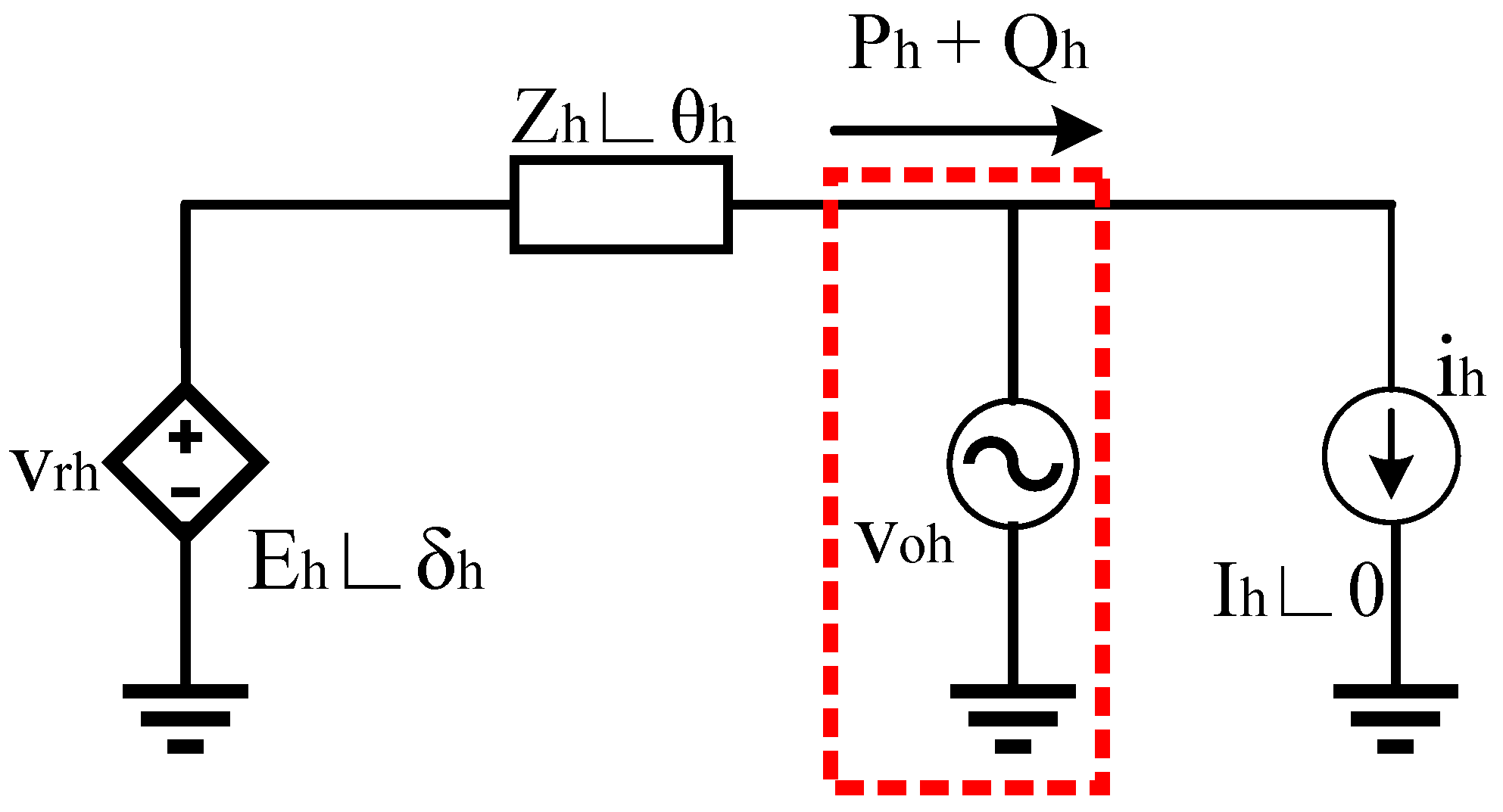
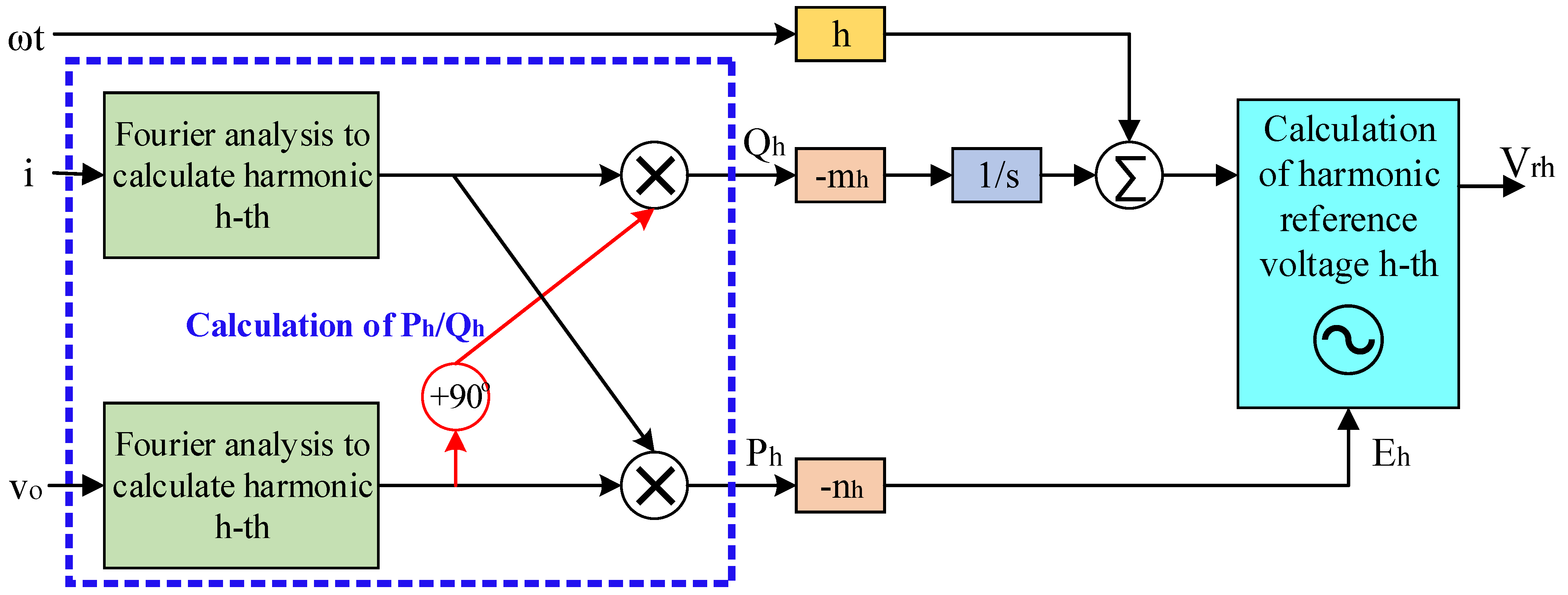
3.1. Harmonic Droop Controller and Voltage Quality Increase

Figure 9 describes the equivalent circuit of an inverter-based DG in the presence of high-frequency harmonics. In general, in the presence of nonlinear loads, the inverter is modeled as a voltage source with coupling impedance Z, and the load is modeled as a combination of voltage and current sources at different frequencies. As a result, the output voltage and current equations are expressed as shown in Equations (33)–(36).

$$v_o=v_{o1}+{{\displaystyle \sum }}_{h=2}^{\infty }{v}_{oh},$$

(33)

$$v_{o1}=\sqrt{2}{V}_{o1}\sin \left({\omega }^{\ast }t\right),$$

(34)

$$v_{oh}=\sqrt{2}{V}_{oh}\sin \left(h{\omega }^{\ast }t+{\phi }_h\right),$$

(35)

$$i={{\displaystyle \sum }}_{h=1}^{\infty }{i}_h,$$

(36)

where ω* is the nominal fundamental frequency of the system, V_o1 is the effective value of the main component of the output voltage, V_oh is the effective value of the h-th component of the output voltage, and φ_h is the phase of the h-th component of the output voltage at time t = 0. The harmonic current is calculated from Equation (37).

$$i_h=\sqrt{2}{I}_h\sin \left(h{\omega }^{\ast }t+{\phi }_h\right).$$

(37)

Equations (33)–(37) of the mathematical model show the effect of nonlinear load and harmonic current in the system. The reference voltage v_r is generally expressed using Equation (38).

$$v_r=v_{r1}+{\displaystyle \sum }_{h=2}^{\infty }{v}_{rh},$$

(38)

$$v_{r1}=\sqrt{2}E\sin \left({\omega }^{\ast }t+\delta \right),$$

(39)

$$v_{rh}=\sqrt{2}{E}_h\sin \left(h{\omega }^{\ast }t+{\delta }_h\right),$$

(40)

where δ is the phase of the main component of the input voltage, and δ_h is the phase of the h-th component of the input voltage at time t = 0. To simplify the mathematical analysis of the circuit in Figure 9, for each harmonic frequency, an equivalent circuit according to Figure 10 is considered and analyzed separately. Then, the response of the system is calculated for each harmonic frequency, and the overall response of the system is obtained using the sum of effects theorem.

For the h-th harmonic effect of the voltage at the output of an inverter-based DG to be close to zero, it is necessary to consider the voltage source v_oh in Figure 10 to be close to zero. That is, the harmonic component is modeled as a current source, i.e., the harmonic power that the v_rh source transmits to the i_h current source through the impedance Z_h. According to Figure 10, the output voltage is calculated from Equation (41).

$$v_{oh}=E_h∟{\delta }_h-Z_h{I}_h∟{\theta }_h=\left(E_h{I}_h\cos {\delta }_h-Z_h{I}_h\cos {\theta }_h\right)+j\left(E_h{I}_h\cos {\delta }_h-Z_h{I}_h\sin {\theta }_h\right).$$

(41)

As a result, the transmitted power is obtained from Equations (42) and (43).

$$P_h=E_h{I}_h\cos {\delta }_h-Z_h{I}_h^2\cos {\theta }_h.$$

(42)

$$Q_h=E_h{I}_h\sin {\delta }_h-Z_h{I}_h^2\cos {\theta }_h.$$

(43)

If the power transmission angle is small, then cos δ ≈ 1 and sin δ ≈ δ. Therefore, Equations (42) and (43) are calculated approximately using Equations (44) and (45).

$$P_h\approx E_h{I}_h-Z_h{I}_h^2\cos {\theta }_h.$$

(44)

$$Q_h=E_h{I}_h{\delta }_h-Z_h{I}_h^2\cos {\theta }_h.$$

(45)

Therefore,

$$P_h~ E_h, Q_h~ {\delta }_h.$$

(46)

The power droop control characteristics for DGs are selected in such a way that negative feedback is established in the active and reactive power control loop of DG. Due to the existence of this negative feedback, the production capacity of DG increases with less production. Therefore, the load demand is divided between DGs according to their capacity. For this purpose, the power droop control relations for harmonic source v_rh are chosen as Equations (47) and (48).

$${\omega }_h=h{\omega }^{\ast }-m_h{Q}_h.$$

(47)

$$E_h=E_h^{\ast }-n_h{P}_h.$$

(48)

P_h and Q_h are the active and reactive powers, respectively, that the inverter-based DG exchanges with the current source i_h; m_h and n_h are the frequency and voltage droop coefficients, respectively, which are calculated similarly to m_i and n_i coefficients. In such a way, the ratio of $m_h{Q}_h$ to $h{\omega }^{\ast }$ is within the permissible range according to the power generation capacity of DGs and the maximum acceptable changes for its frequency.

According to the above explanations, when the output of the voltage sources is connected to a current source through the coupling impedance, the voltage and frequency droop control strategy is independent of the type of coupling impedance, and, for resistive, inductor, and capacitor impedances, the characteristics of Equations (47) and (48) are used. Therefore, by applying this strategy, the controller can be designed in different impedances without the need to check the coupling impedance type of the source, and this makes it easier to design the controllers in the harmonic environment.

To fulfill the v_oh condition, it is necessary to first assume that the active and reactive power that the inverter-based DG exchanges in the h-th harmonic with the harmonic current source i_h is equal to zero. Second, the value of E_h* in Equation (48) should be considered zero. According to the stated contents, the frequency and voltage droop control equations for the h-th harmonic component are obtained from Equations (49) and (50).

$$E_h=-n_h{P}_h.$$

(49)

$${\omega }_h=h{\omega }^{\ast }-m_h{Q}_h.$$

(50)

Now, using the above relationships and Equation (40), the waveform of the h-th component of the reference voltage (v_rh) can be determined. However, in practice, by adding hωt (ωt, the phase of the main component of the reference voltage) and δ which are obtained from the integral −m_hQ_h in Equation (50), the phase of the v_r waveform can be determined. Figure 11 shows the droop controller strategy to determine v_rh. According to Equation (49), the voltage range controller is proportional. In the proportional controller, V_oh is never equal to zero and there is a steady state error. Therefore, according to Figure 11, Equations (51)–(53) are valid.

$$V_{oh}\approx E_h-Z_h{I}_h.$$

(51)

$$E_h=-n_h{P}_h\cong -n_h{V}_{oh}{I}_h.$$

(52)

$$\begin{array}{c}TH{D}_h=\frac{V_{oh}}{V_{o1}}=\frac{Z_h{I}_h}{\left(n_h{I}_h+1\right)E^{\ast }}\\ i_h={\displaystyle \sum }_{j=0}^{N-1}{i}_j{e}^{-2\pi ijk/N}=A_h{e}^{i{\Phi }_h}\\ v_{oh}={\displaystyle \sum }_{j=0}^{N-1}v{o}_j{e}^{-2\pi ijk/N}=A_h{e}^{i{\Phi }_h}\end{array}.$$

(53)

According to Equation (53), THD_h has a direct relationship with the impedance of the h-th harmonic frequency, i.e., the lower the impedance at the h-th harmonic frequency, the lower the THD_h at that frequency. In Figure 11, Fourier analysis is applied to the number of N inputs in the time domain based on moving windows, the output of which will be a frequency spectrum including N points with a known frequency and amplitude. As you can see in Equation (53), harmonic current and voltage can be calculated through Fourier analysis. Here, the range of frequency k can be changed between −(N/2 − 1) and N/2. The output of this transformation is in the form of an amplitude A_h and a phase Φ_h.

On the other hand, V_oh has an inverse relationship with n_h, which is a control parameter. By choosing a larger n_h to the extent that the system remains in a stable state, it is possible to achieve a smaller V_oh and, as a result, a lower THD_h in the output voltage. Subsequently, to correct THD_h, the harmonic droop controllers described above and the modified droop controller are used at the same time. In this way, the amount of voltage required to reduce the output active and reactive power related to each harmonic component are calculated separately by the harmonic controller related to the same component and are added to the reference voltage value of the main component and, thus, the THD of the output voltage is reduced. Figure 12 shows this strategy. Another advantage of using harmonic droop controllers is the accurate sharing of active and reactive power between DGs in addition to reducing THD. This is because, in this case, harmonic active and reactive power (P_h, Q_h) is included in the power-sharing calculations.

The modified droop controller was fully explained to achieve accurate power sharing between inverter-based DGs. Using this controller, the voltage regulation is also improved; as a result, using the harmonic controller, the THD of the output voltage of the inverter is improved with the resistance output impedance. In the next section, by modifying the voltage control loop and combining it with the harmonic droop controller, the quality of the output voltage is improved to a great extent.

3.2. Combination of Harmonic Drop Controller with Virtual Impedance Loop to Correct the THD

A single-phase half-bridge inverter connected to a DC voltage source and an LC filter is shown in Figure 13. In this inverter, PWM control signals are used for alternating output voltage. As can be seen, the control signal u is converted by the PWM converter into a suitable control signal for starting the inverter. For the output impedance of the inverter to be predominantly resistance, it is necessary to measure the output current of inverter i and place it in the control loop. Accordingly, we have

$$u_f=sli+v_i.$$

(54)

$$u=v_r-k_{i}i.$$

(55)

As long as the average value of u_f is almost equal to u in a switching period, the approximate relations in Equation (56) are established.

$$\{\begin{array}{c}{v}_r-k_{i}i=sli-v_o\\ v_o=v_r-\left(k_i+1\right)i\\ \begin{array}{c}{v}_o=v_r-z_o\left(s\right)i\\ z_o\left(s\right)=sl+k_i\end{array}\end{array}.$$

(56)

According to Equation (56), if the gain k_i is chosen large enough, in a wide range of frequencies, the effect of the inductor on the output impedance can be ignored, and the output impedance can be assumed to be almost resistant.

$$z_o\left(s\right)\approx R_o=k_i.$$

(57)

Increasing the k_i gain to achieve the resistive output impedance increases the THD of the output voltage. To improve the quality of the output voltage, the voltage v_o is compared with the reference voltage v_r and is placed in the voltage control loop. According to Figure 13, Equations (58) and (59) are obtained.

$$u=v_r-k_{i}i+k_R\left(s\right)\left(v_r-v_o\right).$$

(58)

$$u_f=sli+v_o.$$

(59)

Here, z_o(s) is the output impedance, which is obtained from Equation (60).

$$z_o\left(s\right)=\frac{sl+k_i}{1+k_R\left(s\right)}.$$

(60)

When the real component of k_R(s) is positive, the resistance and inductor parts of the output impedance are reduced; as a result, the THD of the output voltage is corrected. According to Equation (60), the inductor current feedback increases the output impedance and, as a result, increases the voltage THD; the voltage feedback decreases the output impedance and, as a result, reduces the voltage THD. The k_R(s) block in Figure 13 can be designed in such a way that it has low gain at low frequencies and high gain at high frequencies. As a result, the output impedance at low frequency, especially the fundamental frequency, is predominantly resistive. Furthermore, the output impedance range for harmonic frequencies is a small value that reduces the THD of the output voltage. There are various methods to design the k_R(s) block, among which Equation (61) can be mentioned.

$$k_R\left(s\right)={{\displaystyle \sum }}_{h=3,5,7}\frac{2\mathsf{\zeta }\mathrm{h}\mathsf{\omega }\mathrm{s}}{s^2+2\mathsf{\zeta }\mathrm{h}\mathsf{\omega }\mathrm{s}+{\left(\mathrm{h}\mathsf{\omega }\right)}^2}\times k_h,$$

(61)

where k_h is the gain of Equation (61) at frequency hω, and its phase is equal to zero. Moreover, ζ is the damping coefficient and is usually considered equal to 0.01.

Due to the limitation in choosing the values of n_h and m_h, the harmonic droop controller, despite the reduction in THD of the output voltage, still does not inject the power with the desired quality into the system when feeding sensitive loads. The selection of characteristic coefficients of the harmonic droop controller is based on the capacity of generating harmonic powers of DGs, in other words, DGs reduce the range of harmonic components to a certain extent. Therefore, when feeding sensitive loads, to achieve high power quality, it is necessary to place the harmonic controller in the modified voltage loop. The combination of these two strategies causes the main problems of parallel operation of inverter-based DGs, which are proportional power sharing, accurate voltage regulation, and reduction of output voltage THD, which are solved with the combination of these two strategies.

4. Simulation Results

In this section, to show the efficiency of the proposed controller, simulations are implemented in two different scenarios. In the first scenario, the impact of the proposed techniques on the performance of the controller is evaluated; in the second scenario, the impact of system parameters such as linear, nonlinear, and unbalanced load to the PCC bus, the output impedance of inverters, and the power changes of different inverters are evaluated.

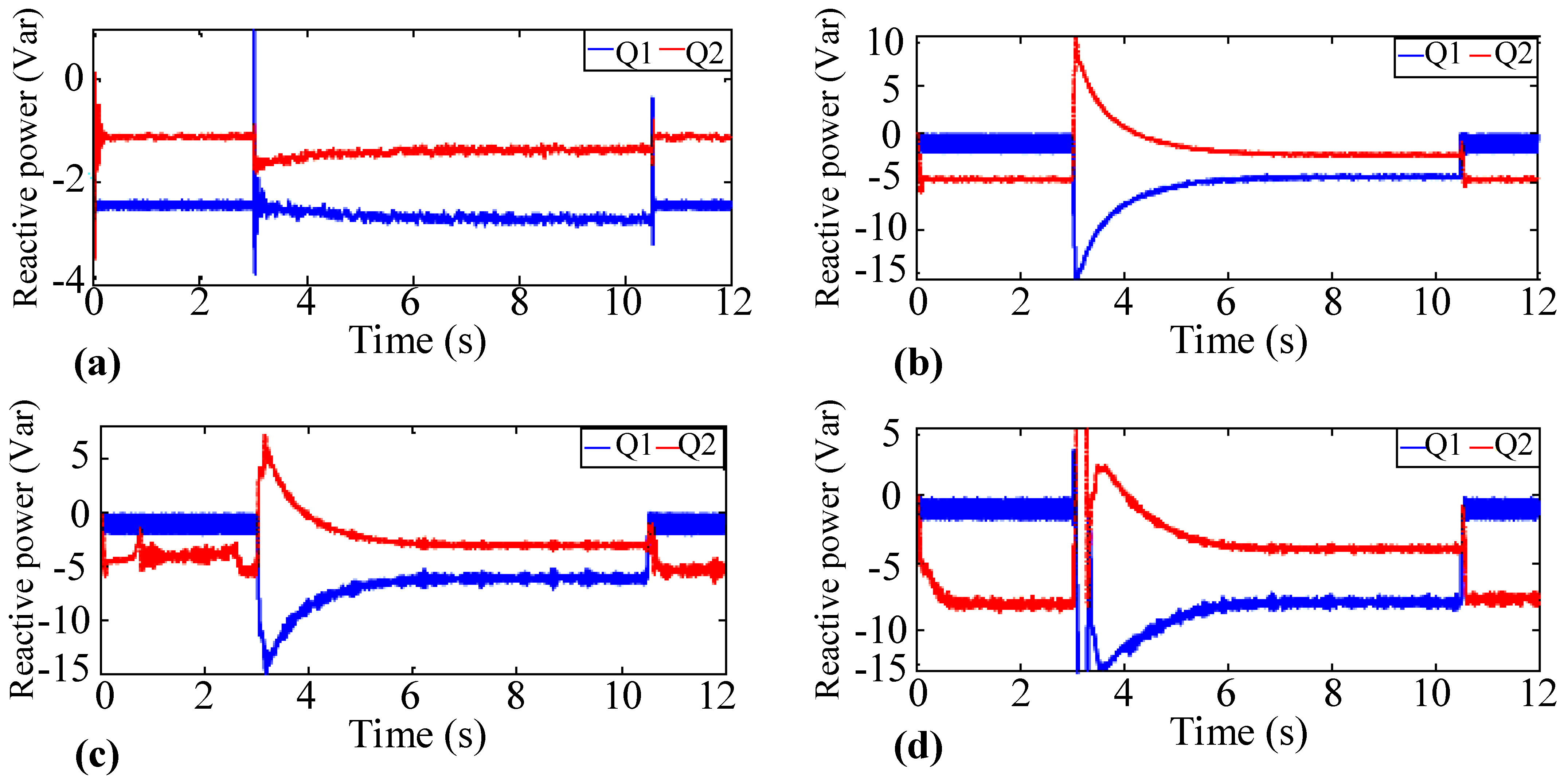
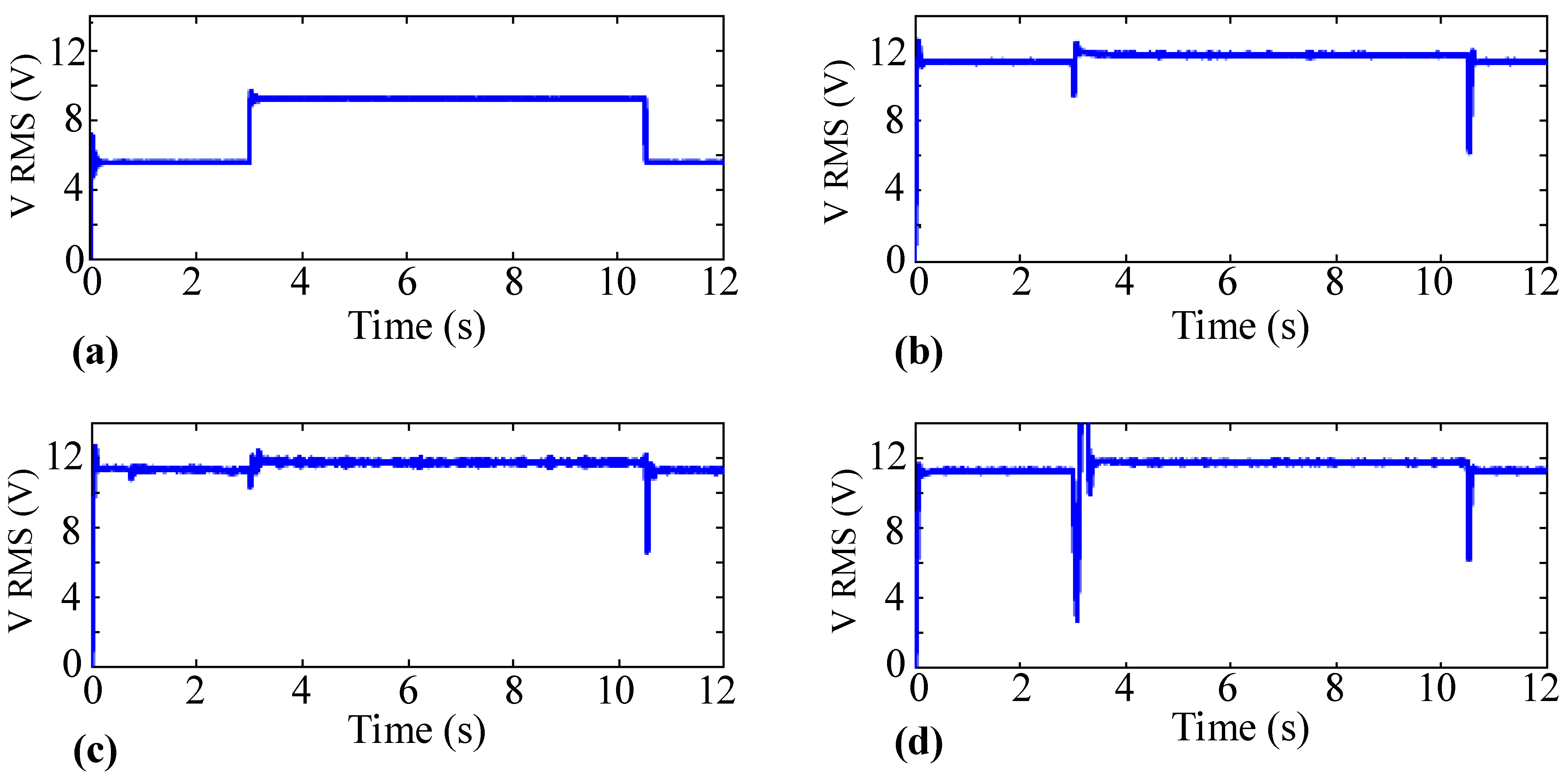
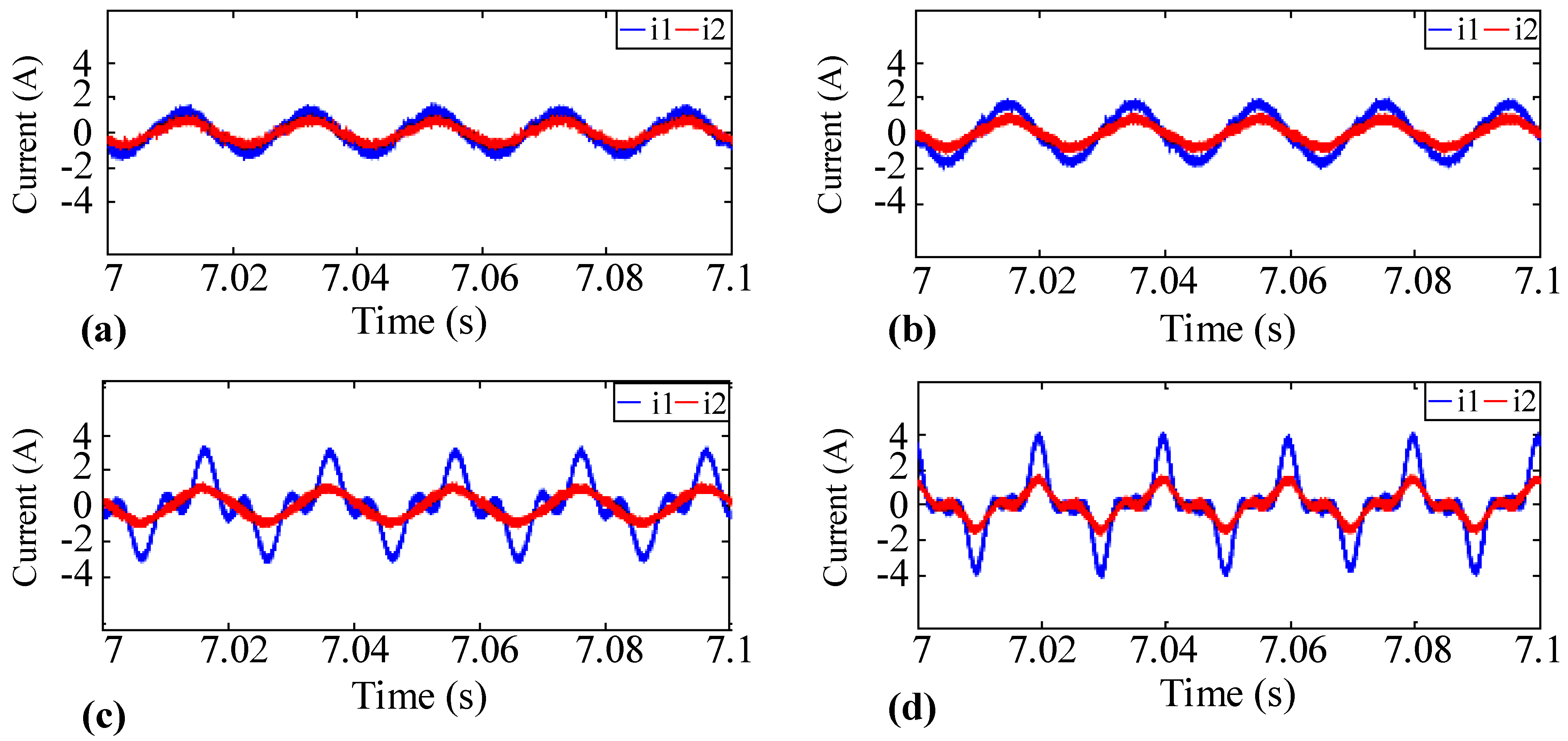
4.1. First Scenario—Strategy 1: Using the Conventional Droop Controller

In this case, the conventional droop control characteristic is used in the droop control block of Figure 13 for inverters with resistive impedance, and the k_R(s) control block is not considered in the control loop. As can be seen in Figure 14a and Figure 15a, active and reactive power sharing is not very accurate, and a large voltage drop is observed at the output of the inverters according to Figure 16a, Figure 17a and Figure 18a. Furthermore, according to Figure 19a, the THD of the output voltage is high and around 29.85% due to the presence of nonlinear load. As a result, by using this droop controller, it is not possible to achieve accurate power sharing between DGs at a ratio of 2:1 and proper voltage regulation at the busload output of inverters.

4.2. First Scenario—Strategy 2: Using a Modified Droop Controller

In this case, the modified droop control characteristic in the droop control block of Figure 13 is used, the gain k_e is selected for both inverters as 20, and the remaining parameters remain unchanged. As Figure 14b and Figure 15b show, using this controller, active and reactive power sharing is performed accurately between DGs. Because the size of the source voltage, unlike the frequency, is a local quantity, it is not possible to accurately share the active power between DGs through the conventional voltage droop characteristic. However, by using the modified droop strategy, the active power between DGs is precisely shared, and the voltage drop caused by the impedance of DGs is compensated for to a large extent.

Active and reactive power values of the steady state for the parallel operation of two inverter-based DGs are shown in

Table 1. Comparison of steady-state values of active and reactive power in the first scenario.

Strategies	Powers
	P1	P2	Q1	Q2
Strategy 1	7.1	3.9	−1.7	−2.8
Strategy 2	11.5	5.7	−4.5	−2.4
Strategy 3	13.7	6.9	−6.4	−3.2
Strategy 4	13.6	6.8	−8	−4

. The effective value of the output voltage compared to the first strategy, according to Figure 16a,b, is improved from 9.2 V to 11.85 V. Therefore, two of the main problems in the parallel operation of inverter-based DGs, which are power sharing and voltage regulation, are solved by using this strategy. Due to the presence of nonlinear loads in the system, the amplitude of the harmonic components of the current is increased; as a result, the THD of the output voltage is increased. Therefore, this controller is not able to solve the problems related to the power quality of parallel inverter-based DGs.

4.3. First Scenario—Strategy 3: Using a Modified and Harmonic Droop Controller

In this case, the third and fifth harmonic droop controller is used simultaneously with the modified controller in the droop control block of Figure 13, in which the reference voltage value (v_r) is equal to the sum of components v_r1, v_r3, and v_r5. Harmonic droop control coefficients n_h and m_h are calculated as 1 and 10 for the third harmonic controller and as 2.1 and 21 for the fifth harmonic controller, while other parameters remain unchanged. The simulation was performed by applying the third strategy, and the results of this strategy are shown in Figure 14c, Figure 15c, Figure 16c, Figure 17c, Figure 18c and Figure 19c. As can be seen in these figures, due to the use of the modified droop controller, according to the droop coefficients of the active and reactive powers, it was accurately shared between DGs in a ratio of 2:1. In this case, as mentioned, since harmonic powers are also included in power sharing between DGs, according to Table 1, active and reactive powers are more precisely divided between DGs. In the previous strategies, due to the presence of nonlinear load in the system, the amplitude of the harmonic components of the current is increased and, as a result, the THD of the output voltage is increased. Using the harmonic droop controller, the quality of the output voltage is somewhat improved and the THD of the output voltage is reduced from 29.70% to 12.55%. Furthermore, the third harmonic THD is reduced from 25% to 12% and the fifth harmonic THD is reduced from 13% to 3%. As expected, by combining the harmonic droop controller strategy with the modified droop control, the quality of the output voltage is improved to some extent.

4.4. First Scenario—Strategy 4: Using the Modified, Harmonic Droop Controller and kR(s) Control Block

In the proposed method, modified and harmonic droop control is used in the droop control block of Figure 13 for inverters with resistive impedance, and the k_R(s) control block is placed in the control loop. Since, in the previous section, the amplitude of the third harmonic component was high, in the k_R(s) block, only the coefficient k_h is used for the third frequency, and its value is designated as 5.3. In this case, care must be taken in selecting the coefficients of n₃ and m₃. According to Figure 14d and Figure 15d, using this combined strategy, the power is accurately divided between DGs.

As can be seen in Figure 16d, there is a slight voltage drop in the voltage output, which indicates proper voltage regulation in the inverter-based DG output. Using the combined strategy, the quality of the output voltage is significantly improved, and the THD of the output voltage is reduced to 6.37%, while the third harmonic THD is reduced from 10.2% to 3%. As expected, the quality of the output voltage is improved with the proposed combined method. Therefore, the main problems of parallel operation of inverter-based DGs, which are power sharing and voltage regulation, as well as THD of the output voltage, are solved using a combination strategy. Moreover, Figure 17 a-d shows the output current changes in the first scenario using the four strategies. To compare the quality of the output voltage in Figure 18 and Figure 19 when using these four types of strategies, the results of THD voltage are given in

Table 2. Comparison of voltage quality in terms of harmonics in the first scenario.

Strategies	Voltage Quality
	THD	THD3	THD5	THD7
Strategy 1	29.85	25.5	12.75	7
Strategy 2	29.70	25.5	12.7	7
Strategy 3	12.55	10.2	3	5.3
Strategy 4	6.37	3	4	2.5

. The blocks used in the third and fourth strategies are only to improve the THD of the output voltage.

In the first scenario, four strategies are investigated in the inverter-based DG voltage control loop. In the first strategy, the conventional droop controller is placed in the voltage control loop to share the power between two inverter-based DGs. To divide the load proportionally between DGs, in the second strategy, a modified droop controller is used in the voltage control loop. In the third strategy, using the harmonic droop controller, the third and fifth harmonic voltages are added to the reference voltage in the voltage control loop; as a result, the THD of the output voltage is reduced.

To significantly improve the quality of the output voltage, in the fourth strategy, in addition to the harmonic droop controller, the k_R(s) block is used in the voltage control loop. In this scenario, the simulation was performed for two half-bridge inverters, as shown in Figure 13, that feed the nonlinear load in parallel. The 9 Ω resistor is connected to the inverters through the full bridge rectifier and filter and acts as a nonlinear load for the system. The values of the inductor and capacitor of the interface filter between the load and the rectifier are 0.15 mH and 1000 mF, respectively. In this case, the droop coefficients n₁ = 0.4, n₂ = 0.8, m₁ = 0.07, and m₂ = 0.14 are adjusted; therefore, it is expected that the load is divided between the DGs in a ratio of 2:1. The switching frequency is 7.5 kHz, and the fundamental frequency is 50 Hz. The effective value of the output voltage is 12 V, and the inverter is designed to have a resistive output impedance in a wide range of frequencies. It should be mentioned that the proper operation of the microgrid in the island mode is explained according to the IEEE 1547.4 standard and is evaluated accordingly. The feedback current gain (k_i1) is set to 2 for the first inverter and k_i2 to 4 for the second inverter. The second inverter feeds the nonlinear load from the beginning, and the first inverter is connected to the system at t = 3; both inverters feed the load in parallel and exit the circuit at t = 10.5.

As mentioned, in the conventional droop controller, to accurately share the load between the parallel inverters, the inverters must have the same conditions; for this purpose, in the proposed method, the droop coefficients of the inverters were chosen differently to show the performance of the proposed controller better than the conventional droop controller. Figure 20 compares the output voltage changes in the first scenario for the proposed controller with the conventional droop controller. For a better display, a difference of 0.01 s was created between the two controllers. As can be seen, less distortion occurred in the voltage waveform with the proposed method, and this difference in inverter coefficients caused the conventional droop controller to not perform properly.

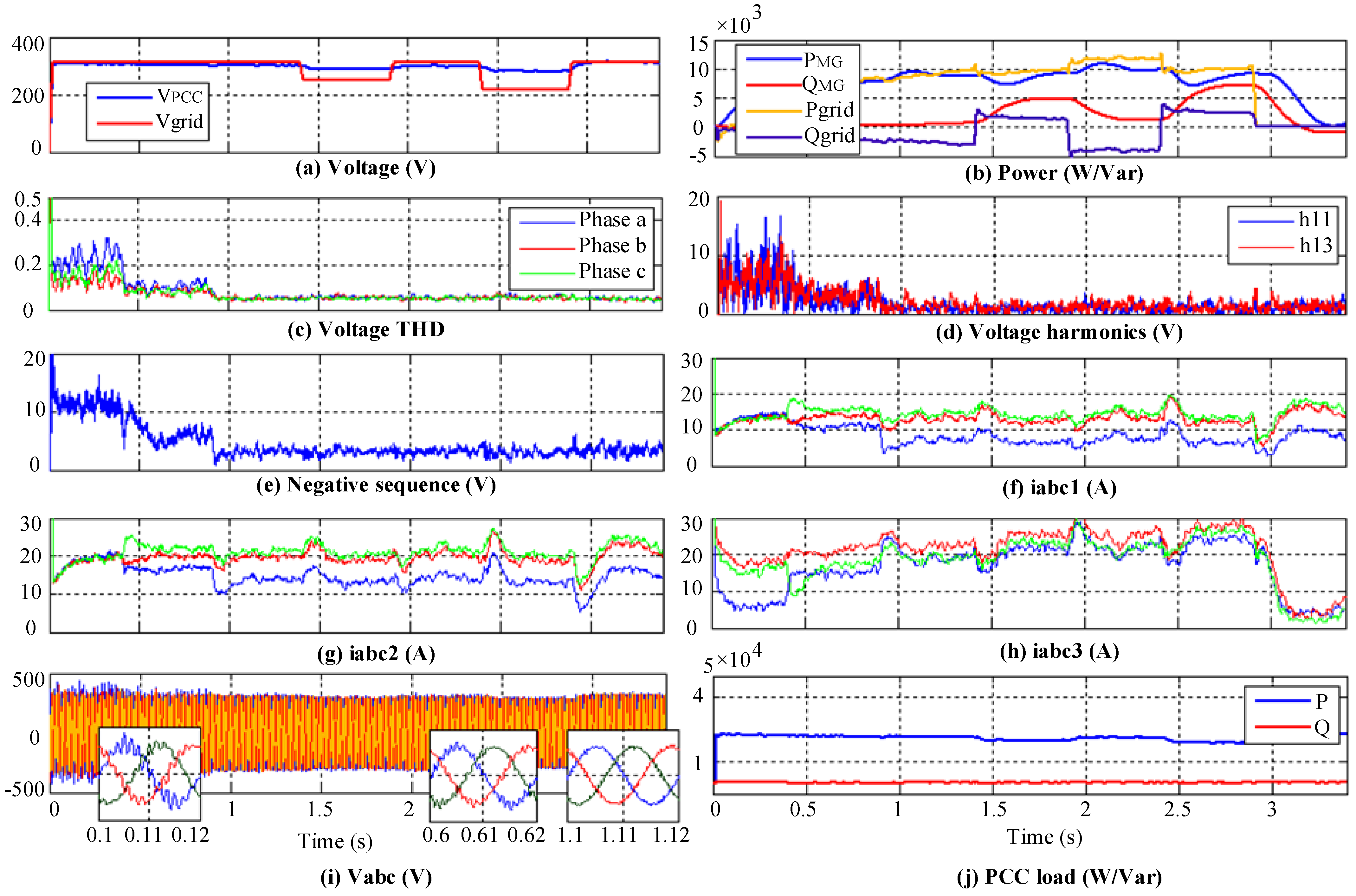
4.5. The Second Scenario: Implementation in Connected and Island Mode from the Grid

In this scenario, the simulation for the sample microgrid in Figure 21 was performed according to the parameters in

Table 3. Microgrid parameters and control system.

Symbol	Parameter	Value
E	Grid voltage amplitude	311 V
Vdc	DC link voltage	650 V
Ω*	Grid fundamental frequency	314 Rad/s
Zload, PCC	Load impedance	20 + j6.5 Ω
ZUL	Unbalance load	50 + j6.5 Ω
Lg, L1f	Filter inductance	0.2, 1.8 mH
Fs	Switching frequency	10 kHz
Zl1, Zl2, Zgrid	Line impedance	j0.47, j0.62, j0.3 Ω
Rv-1, Rv5, Rv7, Rv11	Virtual resistance	9 Ω
Cf	Filter capacitor	25 μF
kp, ki	PI controller coefficient	0.2, 6 W/rd

, in the grid-connected and island mode. The nonlinear load in the third bus was a three-phase diode rectifier with a load of 100 Ω and a filter capacitor of 200 μF. The principles of operation of the three-phase inverter are that this inverter had three single-phase inverter switches, and each switch could be connected to the load terminal. Each switch could connect to three load terminals at the same time. In normal mode, the three keys of this inverter were delayed by 120° to create three-phase AC storage. Therefore, in the second scenario, it was implemented with the assumption of three single-phase controllers.

To create an imbalance, a single-phase load was placed between phases a and b in the PCC bus. In this scenario, the harmonic compensation was evaluated under the influence of the output impedance of DGs, i.e., once without considering the effect of the output impedance of DGs uniformly (participation of DGs with the same priority in compensation), and once by taking into account the effect of the output impedance of DGs; this was conducted in a nonuniform way.

The simulation was performed in seven timesteps, and its results are shown in Figure 21.

Step 1 (0 < t < 0.4s): In this stage, the microgrid is connected to the upstream grid, and all the linear, unbalanced, and nonlinear loads in the buses are in service. The simulation starts with zero initial conditions for DGs and reaches a steady state after passing through the initial transient conditions. The microgrid sends approximately 10 kW of power to the upstream grid and no harmonic compensation is performed.

Step 2 (0.4 s < t < 0.9 s): In this stage, the proposed combined method is activated, and DGs participate in compensating harmonics and voltage imbalance in the same way and with equal capacities, regardless of the output impedance of the inverters.

Step 3 (0.9 s < t < 1.4 s): In this step, compensation is achieved with a nonuniform method and considering the output impedance of the inverters. The THD value of voltage in bus 3 in uncompensated mode is about 17%, which is reduced to 9% in uniform compensation mode. In the nonuniform compensation method, according to Figure 22c, it is reduced to 4%. The waveforms of the 11th and 13th harmonics of the PCC point voltage are shown in Figure 22d. Nonuniform compensation continues from this stage until the end of the simulation stages.

Step 4 (1.4 s < t < 1.9 s): In this stage, a reduction of 0.15 p.u. occurs in the grid voltage range, and the microgrid manages to maintain the microgrid voltage by injecting reactive power of about 4 kVar.

Step 5 (1.9 s < t < 2.4 s): In this stage, the grid voltage returns to normal.

Step 6 (2.4 s < t < 2.9 s): In this stage, a decrease of 0.25 p.u. occurs in the grid voltage range, and the microgrid maintains the microgrid voltage by injecting reactive power of about 7 kVar; however, because this power is more than the capacity of the inverters, the microgrid is disconnected from the grid at the moment of 2.9 s.

Step 7 (2.9 s < t < 3.4 s): At this stage, the reactive power of the microgrid is reduced to 1 kVar to regulate the microgrid voltage, and the microgrid continues to operate as an island. The THD waveform and the voltage harmonics show that the task of compensating for disturbances was successful even in island mode.

5. Conclusions

In this article, a new idea regarding droop controllers with the presence of inverter-based DGs connected to a microgrid in the presence of nonlinear loads was presented. In this structure, the droop controller is modified in such a way that the power is accurately divided between the DGs, and the voltage drop caused by the impedance of the DGs is compensated for. The effect of inverter-based DGs on harmonics injected into the microgrid was studied. Considering that inverter-based DGs without control schemes can have a destructive effect in creating voltage and current harmonics in the connection to the microgrid, in this article, a combined power-sharing strategy based on the frequency/voltage control loop method and harmonic droop controller was provided. By applying the proposed strategy and modifying the voltage control loop, the performance of power sharing in the system was improved, and a significant improvement in voltage harmonics and injection current to the microgrid was achieved. For future studies, this proposed method can be used effectively to reduce voltage harmonics in parallel operation of inverters in islanded microgrids, as well as on grid-connected systems.

References

1. Masoud, D.; Najafi, M.; Esmaeilbeig, M. Calculating the locational marginal price and solving optimal power flow problem based on congestion management using GA-GSF algorithm. Electr. Eng. 2020, 102, 1549–1566. [Google Scholar]
2. Masoud, D.; Najafi, M.; Esmaeilbeig, M. Reducing LMP and resolving the congestion of the lines based on placement and optimal size of DG in the power network using the GA-GSF algorithm. Electr. Eng. 2021, 103, 1279–1306. [Google Scholar]
3. Daniel, H.; Ratasich, D.; Krammer, L.; Jantsch, A. A methodology for resilient control and monitoring in smart grids. In Proceedings of the 2020 IEEE International Conference on Industrial Technology (ICIT), Buenos Aires, Argentina, 26–28 February 2020; pp. 589–594. [Google Scholar]
4. Andrew, D.S.; Alcaraz, C.; Hatziargyriou, N.D. Classifying resilience approaches for protecting smart grids against cyber threats. Int. J. Inf. Secur. 2022, 21, 1189–1210. [Google Scholar]
5. Dileep, G. A survey on smart grid technologies and applications. Renew. Energy 2020, 146, 2589–2625. [Google Scholar]
6. Hosseinimoghadam, S.M.; Roghanian, H.; Dashtdar, M.; Razavi, S.M. Power-sharing control in an islanded microgrid using virtual impedance. In Proceedings of the 2020 8th International Conference on Smart Grid (icSmartGrid), Paris, France, 17–19 June 2020; pp. 73–77. [Google Scholar]
7. Hosseinimoghadam, S.M.; Dashtdar, M.; Dashtdar, M.; Roghanian, H. Security control of islanded micro-grid based on adaptive neuro-fuzzy inference system. Sci. Bull. Ser. C Electr. Eng. Comput. Sci. 2020, 1, 189–204. [Google Scholar]
8. Masoud, D.; Dashtdar, M. Voltage and frequency control of islanded micro-grid based on battery and MPPT coordinated control. Int. J. Electr. Comput. Sci. (IJECS) 2020, 2, 1–19. [Google Scholar]
9. Shaheed Bin, M.N.; Sozer, Y.; Chowdhury, S.; De Abreu-Garcia, J.A. A novel decentralized adaptive droop control technique for DC microgrids based on integrated load condition processing. In Proceedings of the 2020 IEEE Energy Conversion Congress and Exposition (ECCE), Virtual, 11–15 October 2020; pp. 2095–2100. [Google Scholar]
10. Masoud, D.; Nazir, M.S.; Hosseinimoghadam, S.M.S.; Bajaj, M. Improving the sharing of active and reactive power of the islanded microgrid based on load voltage control. Smart Sci. 2021, 10, 142–157. [Google Scholar]
11. Zhang, Y.; Qu, X.; Tang, M.; Yao, R.; Chen, W. Design of nonlinear droop control in DC microgrid for desired voltage regulation and current sharing accuracy. IEEE J. Emerg. Sel. Top. Circuits Syst. 2021, 11, 168–175. [Google Scholar] [CrossRef]
12. Hosseinimoghadam, S.M.S.; Dashtdar, M.; Dashtdar, M. Improving the sharing of reactive power in an islanded microgrid based on adaptive droop control with virtual impedance. Autom. Control Comput. Sci. 2021, 55, 155–166. [Google Scholar] [CrossRef]
13. Saeed, P.; Blaabjerg, F.; Palensky, P. Incorporating power electronic converters reliability into modern power system reliability analysis. IEEE J. Emerg. Sel. Top. Power Electron. 2020, 9, 1668–1681. [Google Scholar]
14. Majid, D.; Dashtdar, M. Voltage control in distribution networks in presence of distributed generators based on local and coordinated control structures. Sci. Bull. Electr. Eng. Fac. 2019, 19, 21–27. [Google Scholar]
15. Lasantha, M.; Sguarezi, A.; Bryant, J.S.; Gu, M.; Conde, D.R.; Cunha, R. Power system stability with power-electronic converter interfaced renewable power generation: Present issues and future trends. Energies 2020, 13, 3441. [Google Scholar]
16. Guo, Y.; Lu, X.; Chen, L.; Zheng, T.; Wang, J.; Mei, S. Functional-rotation-based active dampers in AC microgrids with multiple parallel interface inverters. IEEE Trans. Ind. Appl. 2018, 54, 5206–5215. [Google Scholar] [CrossRef]
17. Guo, Y.; Chen, L.; Lu, X.; Wang, J.; Zheng, T.; Mei, S. Region-Based Stability Analysis of Active Dampers in AC Microgrids with Multiple Parallel Interface Inverters. In Proceedings of the 2019 IEEE Applied Power Electronics Conference and Exposition (APEC), Anaheim, CA, USA, 17–21 March 2019; pp. 1098–1101. [Google Scholar]
18. Wang, S.; Liu, Z.; Liu, J.; Boroyevich, D.; Burgos, R. Small-signal modeling and stability prediction of parallel droop-controlled inverters based on terminal characteristics of individual inverters. IEEE Trans. Power Electron. 2019, 35, 1045–1063. [Google Scholar] [CrossRef]
19. Helmo, K.M.-P.; Burgos-Mellado, C.; Bonaldo, J.P.; Rodrigues, D.T.; Quintero, J.S.G. Cooperative control of power quality compensators in microgrids. In Proceedings of the 2021 IEEE Green Technologies Conference (GreenTech), Denver, CO, USA, 7–9 April 2021; pp. 380–386. [Google Scholar]
20. Jayant, S.; Sundarabalan, C.K.; Sitharthan, R.; Balasundar, C.; Srinath, N.S. Power quality enhancement in microgrid using adaptive affine projection controlled medium voltage distribution static compensator. Sustain. Energy Technol. Assess. 2022, 52, 102185. [Google Scholar]
21. Masoud, D.; Flah, A.; El-Bayeh, C.Z.; Tostado-Véliz, M.; Al Durra, A.; Aleem, S.H.A.; Ali, Z.M. Frequency control of the islanded microgrid based on optimized model predictive control by PSO. IET Renew. Power Gener. 2022, 16, 2088–2100. [Google Scholar]
22. Naji, A.; Jasim, B.H.; Issa, W.; Anvari-Moghaddam, A.; Blaabjerg, F. A new robust control strategy for parallel operated inverters in green energy applications. Energies 2020, 13, 3480. [Google Scholar]
23. Aimée, I.; Saulo, M.J.; Wekesa, C.W. Arctan-Based Robust Droop Control Technique for Accurate Power-Sharing in a Micro-Grid. Eng. Technol. Appl. Sci. Res. 2022, 12, 8259–8265. [Google Scholar]
24. Majid, D.; Dashtdar, M. Power control in an islanded microgrid using virtual impedance. Sci. Bull. Electr. Eng. Fac. 2020, 20, 44–49. [Google Scholar]
25. Harsh, D.P.; Gandhi, P.; Darji, P. PV-Array-Integrated UPQC for Power Quality Enhancement and PV Power Injection. In Recent Advances in Power Electronics and Drives; Springer: Singapore, 2022; pp. 433–449. [Google Scholar]
26. Akhil, G. Power quality evaluation of photovoltaic grid interfaced cascaded H-bridge nine-level multilevel inverter systems using D-STATCOM and UPQC. Energy 2022, 238, 121707. [Google Scholar]
27. Masoud, D.; Bajaj, M.; Hosseinimoghadam, S.M.S.; Sami, I.; Choudhury, S.; Rehman, A.U.; Goud, B.S. Improving voltage profile and reducing power losses based on reconfiguration and optimal placement of UPQC in the network by considering system reliability indices. Int. Trans. Electr. Energy Syst. 2021, 31, e13120. [Google Scholar]
28. Dahiya, S. Distributed control for DC microgrid based on optimized droop parameters. IETE J. Res. 2020, 66, 192–203. [Google Scholar]
29. Ahmet, K.; Seker, M.E. Distributed control of microgrids. In Microgrid Architectures, Control and Protection Methods; Springer: Cham, Switzerland, 2020; pp. 403–422. [Google Scholar]
30. Ahmed, J.; Mustafa, M.W.; Rasid, M.M.; Anjum, W.; Ayub, S. Salp swarm optimization algorithm-based controller for dynamic response and power quality enhancement of an islanded microgrid. Processes 2019, 7, 840. [Google Scholar]
31. Masoud, D.; Dashtdar, M. Voltage-frequency control (vf) of islanded microgrid based on battery and MPPT control. Am. J. Electr. Comput. Eng. 2020, 4, 35–48. [Google Scholar]
32. Amgad, E.S.; Arafah, S.H.; Salim, O.M. Power quality enhancement of grid-islanded parallel microsources using new optimized cascaded level control scheme. Int. J. Electr. Power Energy Syst. 2022, 140, 108063. [Google Scholar]
33. He, J.; Du, L.; Yuan, S.; Zhang, C.; Wang, C. Supply voltage and grid current harmonics compensation using multi-port interfacing converter integrated into two-AC-bus grid. IEEE Trans. Smart Grid 2018, 10, 3057–3070. [Google Scholar] [CrossRef]
34. Emin, A.M.; Ahmed, S. Control hardware-in-the-loop for voltage controlled inverters with unbalanced and non-linear loads in stand-alone photovoltaic (PV) islanded microgrids. In Proceedings of the 2020 IEEE Energy Conversion Congress and Exposition (ECCE), Detroit, MI, USA, 11–15 October 2020; pp. 2431–2438. [Google Scholar]
35. Mousazadeh, M.S.Y.; Jalilian, A.; Savaghebi, M.; Guerrero, J.M. Coordinated control of multifunctional inverters for voltage support and harmonic compensation in a grid-connected microgrid. Electr. Power Syst. Res. 2018, 155, 254–264. [Google Scholar] [CrossRef] [Green Version]
36. Alonso, S.; Matheus, A.; Brandao, D.I.; Caldognetto, T.; Marafão, F.P.; Mattavelli, P. A selective harmonic compensation and power control approach exploiting distributed electronic converters in microgrids. Int. J. Electr. Power Energy Syst. 2020, 115, 105452. [Google Scholar] [CrossRef]
37. Hadi, A.M.; Gholipour, E.; Hooshmand, R. Voltage quality enhancement in islanded microgrids with multi-voltage quality requirements at different buses. IET Gener. Transm. Distrib. 2018, 12, 2173–2180. [Google Scholar]
38. Hussain, E.A.; ElDesouky, A.A.; Omar, A.I.; Saad, M.A. Operation control, energy management, and power quality enhancement for a cluster of isolated microgrids. Ain Shams Eng. J. 2022, 13, 101737. [Google Scholar]
39. Maddala, U.; Prasad, A.D. Power Quality Improvement with Multilevel Inverter Based IPQC for Microgrid. Int. J. Mod. Trends Sci. Technol. 2019, 5, 39–43. [Google Scholar]
40. Goharshenasan, K.P.; Joorabian, M.; Seifossadat, S.G. Smart grid realization with introducing unified power quality conditioner integrated with DC microgrid. Electr. Power Syst. Res. 2017, 151, 68–85. [Google Scholar]
41. Cheng, I.C.; Chen, Y.-C.; Chin, Y.-C.; Chen, C.-H. Integrated power-quality monitoring mechanism for microgrid. IEEE Trans. Smart Grid 2018, 9, 6877–6885. [Google Scholar] [CrossRef]
42. Sachin, D.; Singh, B. Performance analysis of solar PV array and battery integrated unified power quality conditioner for microgrid systems. IEEE Trans. Ind. Electron. 2020, 68, 4027–4035. [Google Scholar]
43. Nashitah, A.; Raza, S.; Ali, S.; Bhatti, M.K.L.; Zahra, S. Harmonic power sharing and power quality improvement of droop controller based low voltage islanded microgrid. In Proceedings of the 2019 International Symposium on Recent Advances in Electrical Engineering (RAEE), Islamabad, Pakistan, 28–29 August 2019; Volume 4, pp. 1–6. [Google Scholar]
44. Yassuda, Y.D.; Vechiu, I.; Gaubert, J.-P. A review of hierarchical control for building microgrids. Renew. Sustain. Energy Rev. 2020, 118, 109523. [Google Scholar]
45. Zhirong, Z.; Yi, H.; Zhai, H.; Zhuo, F.; Wang, Z. Harmonic power sharing and PCC voltage harmonics compensation in islanded microgrids by adopting virtual harmonic impedance method. In Proceedings of the IECON 2017-43rd Annual Conference of the IEEE Industrial Electronics Society, Beijing, China, 29 October–1 November 2017; pp. 263–267. [Google Scholar]
46. Fei, D.; Petucco, A.; Mattavelli, P.; Zhang, X. An enhanced current sharing strategy for islanded ac microgrids based on adaptive virtual impedance regulation. Int. J. Electr. Power Energy Syst. 2022, 134, 107402. [Google Scholar]
47. Wang, Z.; Chen, Y.; Li, X.; Xu, Y.; Wu, W.; Liao, S.; Wang, H.; Cao, S. Adaptive Harmonic Impedance Reshaping Control Strategy Based on a Consensus Algorithm for Harmonic Sharing and Power Quality Improvement in Microgrids With Complex Feeder Networks. IEEE Trans. Smart Grid 2021, 13, 47–57. [Google Scholar] [CrossRef]
48. Liu, B.; Liu, Z.; Liu, J.; An, R.; Zheng, H.; Shi, Y. An adaptive virtual impedance control scheme based on small-AC-signal injection for unbalanced and harmonic power sharing in islanded microgrids. IEEE Trans. Power Electron. 2019, 34, 12333–12355. [Google Scholar] [CrossRef]
49. Zhang, H.; Kim, S.; Sun, Q.; Zhou, J. Distributed adaptive virtual impedance control for accurate reactive power sharing based on consensus control in microgrids. IEEE Trans. Smart Grid 2016, 8, 1749–1761. [Google Scholar] [CrossRef]
50. Yu, H.; Awal, M.A.; Tu, H.; Du, Y.; Lukic, S.; Husain, I. A virtual impedance scheme for voltage harmonics suppression in virtual oscillator controlled islanded microgrids. In Proceedings of the 2020 IEEE Applied Power Electronics Conference and Exposition (APEC), New Orleans, LA, USA, 15–19 March 2020; pp. 609–615. [Google Scholar]
51. Wu, X.; Shen, C.; Iravani, R. Feasible range and optimal value of the virtual impedance for droop-based control of microgrids. IEEE Trans. Smart Grid 2016, 8, 1242–1251. [Google Scholar] [CrossRef]
52. Huang, P.-H.; Vorobev, P.; Al Hosani, M.; Kirtley, J.L.; Turitsyn, K. Plug-and-play compliant control for inverter-based microgrids. IEEE Trans. Power Syst. 2019, 34, 2901–2913. [Google Scholar] [CrossRef]
Figure 1. The general structure of microgrid control.
Mathematics 11 00172 g001
Figure 2. Details of the primary and secondary controller of the microgrid.
Mathematics 11 00172 g002
Figure 3. Small signal model of frequency distributed controller for DGk.
Mathematics 11 00172 g003
Figure 4. Small signal model of voltage distributed controller for DGk.
Mathematics 11 00172 g004
Figure 5. Compensator workload controller structure.
Mathematics 11 00172 g005
Figure 6. Equivalent circuit of two inverters connected to the grid.
Mathematics 11 00172 g006
Figure 7. Conventional droop control method.
Mathematics 11 00172 g007
Figure 8. Modified droop control system.
Mathematics 11 00172 g008
Figure 9. Inverter-based DG equivalent circuit connected to the load.
Mathematics 11 00172 g009
Figure 10. The equivalent circuit of the inverter is related to the h-th harmonic frequency.
Mathematics 11 00172 g010
Figure 11. Proposed droop controller to reduce the h-th harmonic of the voltage.
Mathematics 11 00172 g011
Figure 12. Droop controller with several harmonic droop controllers.
Mathematics 11 00172 g012
Figure 13. Modifying the voltage control loop to create the resistance coupling impedance and increase the voltage quality.
Mathematics 11 00172 g013
Figure 14. Reactive power changes in the first scenario using (a) the first strategy, (b) the second strategy, (c) the third strategy, and (d) the fourth strategy.
Mathematics 11 00172 g014
Figure 15. Active power changes in the first scenario using (a) the first strategy, (b) the second strategy, (c) the third strategy, and (d) the fourth strategy.
Mathematics 11 00172 g015
Figure 16. Effective voltage changes in the first scenario using (a) the first strategy, (b) the second strategy, (c) the third strategy, and (d) the fourth strategy.
Mathematics 11 00172 g016
Figure 17. Output current changes in the first scenario using (a) the first strategy, (b) the second strategy, (c) the third strategy, and (d) the fourth strategy.
Mathematics 11 00172 g017
Figure 18. Output voltage changes in the first scenario using (a) the first strategy, (b) the second strategy, (c) the third strategy, and (d) the fourth strategy.
Mathematics 11 00172 g018
Figure 19. THD changes the output voltage in the first scenario using (a) the first strategy, (b) the second strategy, (c) the third strategy, and (d) the fourth strategy.
Mathematics 11 00172 g019
Figure 20. Comparison of output voltage changes in the first scenario using the conventional droop controller and the proposed controller.
Mathematics 11 00172 g020
Figure 21. Three-bus microgrid under study.
Mathematics 11 00172 g021
Figure 22. The results of the second scenario: (a) peak voltage amplitude of the grid phase and PCC bus; (b) grid power and microgrid power; (c) amount of voltage THD in the PCC bus; (d) 13th and 11th harmonic amplitude of voltage in PCC bus; (e) amplitude of negative sequence voltage at PCC bus; (f) effective output currents of inverter 1; (g) effective output currents of inverter 2; (h) effective output currents of inverter 3; (i) instantaneous PCC bus voltages; (j) power of PCC bus loads.
Mathematics 11 00172 g022