Study on Convex Resource Allocation Scheduling with a Time-Dependent Learning Effect

Abstract

In classical schedule problems, the actual processing time of a job is a fixed constant, but in the actual production process, the processing time of a job is affected by a variety of factors, two of which are the learning effect and resource allocation. In this paper, single-machine scheduling problems with resource allocation and a time-dependent learning effect are investigated. The actual processing time of a job depends on the sum of normal processing times of previous jobs and the allocation of non-renewable resources. With the convex resource consumption function, the goal is to determine the optimal schedule and optimal resource allocation. Three problems arising from two criteria (i.e., the total resource consumption cost and the scheduling cost) are studied. For some special cases of the problems, we prove that they can be solved in polynomial time. More generally, we propose some accurate and intelligent algorithms to solve these problems.

1. Introduction

In many real-world industrial processes, job (task) processing times may be variable due to learning effects or resource allocation. Learning effects appear in, for example, the way that workers’ repeated processing of similar jobs improves their skills (see Azzouz et al. [1], Sun et al. [2], Zhao [3], Wang et al. [4], Chen et al. [5], Ren et al. [6], Wang et al. [7]). The processing times of jobs can be controlled by allocating a common limited resource, such as fuel, the financial budget, energy, or manpower (see Guan et al. [8], Wang and Cheng [9], Shabtay and Steiner [10], Zhang et al. [11], Wang et al. [12], Wang et al. [13], Liu and Wang [14]).

In addition, in many real-life situations, the simultaneous occurrence of learning effects and resource allocation can be found; e.g., in the chemical industry. Recently, Lu et al. [15] explored single-machine scheduling with learning effects, group technology, and resource allocation. The objective was to minimize the makespan subject to limited resource availability. To solve the problem, the authors proposed heuristic and branch-and-bound algorithms. Wang et al. [16] studied the resource allocation scheduling problem with learning and deterioration effects with a single machine. For linear resource allocation, they showed that some regular objective function minimizations can be solved in polynomial time. Liu and Jiang [17] considered due date assignment scheduling problems with learning effects and resource allocation. Zhao [18] addressed due window assignment flow shop scheduling problems with learning effects and resource allocation. Wang et al. [19] considered single-machine resource allocation scheduling with truncated learning effects. For the scheduling cost (i.e., the total weighted completion time) and total resource consumption cost, they provided a bicriteria analysis. They proved that some special cases of the problem are solvable in polynomial time. To solve the problem more generally, they proposed a heuristic and a branch-and-bound algorithm. Yan et al. [20] studied single-machine group scheduling with resource allocation and learning effects. For the minimization of the total completion time subject to limited resource availability, they proposed heuristic, tabu search, and branch-and-bound algorithms.

Biskup [21] considered the position-dependent learning effect, i.e., for which the actual processing time of job ${\dot{J}}_j$ in position r is $p_{jr}^A={\overline{p}}_j{r}^{\alpha }$, where ${\overline{p}}_j$ is the normal processing time of job ${\dot{J}}_j$, and $\alpha \le 0$ is the learning factor. Kuo and Yang [22] studied the time-dependent learning effect; i.e., $p_{jr}^A={\overline{p}}_j{(1+{\sum }_{h=1}^{r-1}{\overline{p}}_{\left[h\right]})}^{\alpha }$, where $\alpha \le 0$ is the learning factor and $\left[h\right]$ denotes a job scheduled in the hth position. Wang et al. [23] studied the following model: $p_{jr}^A\left({\tilde{u}}_j\right)={\left(\frac{{\overline{p}}_j{r}^a}{{\tilde{u}}_j}\right)}^{\beta },$ where $\beta >0$ is a given constant, and ${\tilde{u}}_j$ is the resource allocated to the job ${\dot{J}}_j$. The above articles considered the resource allocation scheduling problem with position-dependent learning effects. However, in general, there are two approaches to modeling the learning effect: one is the position-dependent learning effect, and the other is the time-dependent (sum-of-processing-time) learning effect (Azzouz et al. [1]). Hence, in this paper, the work of resource allocation scheduling is continued by researching the time-dependent learning effect (see Table 1). This paper’s contributions and novelties are as follows:

Table 1. Models studied.

References	Scheduling Problem	Time Complexity
Biskup [21]	$1\left|p_{jr}^A={\overline{p}}_j{r}^{\alpha }\right|{\sum }_{j=1}^{\check{n}}{\delta }_1{E}_j+{\delta }_2{T}_j+{\delta }_3{C}_j$	$O\left(n^3\right)$
	$1\left|p_{jr}^A={\overline{p}}_j{r}^{\alpha }\right|{\sum }_{j=1}^{\check{n}}{C}_j$	$O(nlog(n\left)\right)$
Kuo and Yang [22]	$1\left|p_{jr}^A={\overline{p}}_j{(1+{\sum }_{h=1}^{r-1}{\overline{p}}_{\left[h\right]})}^{\alpha }\right|{\sum }_{j=1}^{\check{n}}{C}_j$	$O(nlog(n\left)\right)$
Wang et al. [23]	$1\left|p_{jr}^A\left({\tilde{u}}_j\right)={\left(\frac{{\overline{p}}_j{r}^a}{{\tilde{u}}_j}\right)}^{\beta }\right|{\delta }_1{C}_{max}+{\delta }_{2}TC+{\delta }_{3}TADC{\delta }_4{\sum }_{j=1}^{\check{n}}{G}_j{u}_j$	$O(nlog(n\left)\right)$
	$1\left|p_{jr}^A\left({\tilde{u}}_j\right)={\left(\frac{{\overline{p}}_j{r}^a}{{\tilde{u}}_j}\right)}^{\beta }\right|{\delta }_1{C}_{max}+{\delta }_{2}TW+{\delta }_{3}TADW{\delta }_4{\sum }_{j=1}^{\check{n}}{G}_j{u}_j$	$O(nlog(n\left)\right)$
This article	$1\left|p_{jr}^A\left({\tilde{u}}_j\right)={\left(\frac{{\overline{p}}_j{(1+{\sum }_{h=1}^{r-1}{\overline{p}}_{\left[h\right]})}^{\alpha }}{{\tilde{u}}_j}\right)}^{\beta }\right|\delta {\sum }_{j=1}^{\check{n}}{\vartheta }_j{p}_{\left[j\right]}^A+\eta {\sum }_{j=1}^{\check{n}}{g}_{\left[j\right]}{\tilde{u}}_{\left[j\right]}$	Conjecture NP-hard
	$1\left|p_{jr}^A\left({\tilde{u}}_j\right)={\left(\frac{{\overline{p}}_j{(1+{\sum }_{h=1}^{r-1}{\overline{p}}_{\left[h\right]})}^{\alpha }}{{\tilde{u}}_j}\right)}^{\beta },{\sum }_{j=1}^{\check{n}}{g}_{\left[j\right]}{\tilde{u}}_{\left[j\right]}\le \breve{U}\right|{\sum }_{j=1}^{\check{n}}{\vartheta }_j{p}_{\left[j\right]}^A$	Conjecture NP-hard
	$1\left|p_{jr}^A\left({\tilde{u}}_j\right)={\left(\frac{{\overline{p}}_j{(1+{\sum }_{h=1}^{r-1}{\overline{p}}_{\left[h\right]})}^{\alpha }}{{\tilde{u}}_j}\right)}^{\beta },{\sum }_{j=1}^{\check{n}}{\vartheta }_j{p}_{\left[j\right]}^A\le \breve{V}\right|{\sum }_{j=1}^{\check{n}}{g}_{\left[j\right]}{\tilde{u}}_{\left[j\right]}$	Conjecture NP-hard

• Single-machine scheduling with convex resource allocation and a time-dependent learning effect is modeled and studied;
• The solution algorithms for three versions of the total resource consumption cost and the scheduling cost are presented;
• The computational results of the proposed algorithms are analyzed.

The paper is organized as follows. Section 2 formulates the model. Section 3 gives the basic properties of the problems. Section 4 describes the solution algorithms developed to solve the problems. Section 5 focused on the computational experiments with the algorithms. Section 6 presents the conclusions.

2. Problem Statement

In this paper, the notations used are listed in Table 2, and we consider the problem of scheduling $\check{n}$ jobs ${\dot{J}}_1,{\dot{J}}_2,\dots {\dot{J}}_{\check{n}}$ on a single machine, with all the jobs available at time 0. If the job schedule is ${\dot{J}}_1,{\dot{J}}_2,{\dot{J}}_3,\dots {\dot{J}}_{\check{n}}$, then the Gantt chart of the single-machine scheduling is as in Figure 1:

Table 2. Notations.

Notation	Meaning
$\check{n}$	the number of jobs
${\dot{J}}_j$	the jth job
${\dot{J}}_{\left[j\right]}$	the job scheduled in the jth position
${\overline{p}}_j$	the normal processing time of job ${\dot{J}}_j$
${\overline{p}}_{\left[h\right]}$	the normal processing time of the job scheduled in the hth position
$p_{jr}^A$	the actual processing time of job ${\dot{J}}_j$ in position r
$\alpha$	the learning factor
${\tilde{u}}_j\left({\tilde{u}}_{\left[j\right]}\right)$	the resource allocated to job ${\dot{J}}_j$ (${\dot{J}}_j$)
$C_{\left[j\right]}$ ($C_j$)	the completion time of job ${\dot{J}}_{\left[j\right]}$ (${\dot{J}}_j$)
$p_{\left[j\right]}^A$ ($p_j^A$)	the actual processing time of job ${\dot{J}}_{\left[j\right]}$ (${\dot{J}}_j$)
$g_j\left(g_{\left[j\right]}\right)$	the cost when allocating unit resource to job
${\vartheta }_j$	the position-dependent (but job-independent) weight (cost) of the jth job
$C_{max}$	the makespan of all jobs
$TADC$	the total absolute differences in completion times
$TADW$	the total absolute differences in waiting times
$\beta$ ($\delta$, $\eta )$	the given constant

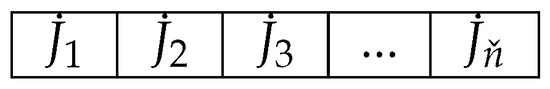
Figure 1. Gantt chart of the problem.

In this paper, the model we consider is given as follows

$$p_{jr}^A\left({\tilde{u}}_j\right)={\left(\frac{{\overline{p}}_j{(1+{\sum }_{h=1}^{r-1}{\overline{p}}_{\left[h\right]})}^{\alpha }}{{\tilde{u}}_j}\right)}^{\beta },$$

(1)

where $\alpha \le 0$ is the learning factor, and $\beta >0$ is a given constant. The goal of this article is to determine the optimal schedule and optimal resource allocation. The first problem of this paper is to minimize

$$F\left({\tilde{u}}_{\left[j\right]}\right)=\delta \sum _{j=1}^{\check{n}}{\vartheta }_j{p}_{\left[j\right]}^A+\eta \sum _{j=1}^{\check{n}}{g}_{\left[j\right]}{\tilde{u}}_{\left[j\right]}.$$

(2)

Using the three-field notation, the first problem (denoted by $\overline{P1}$) can be denoted as

$$1\left|p_{jr}^A\left({\tilde{u}}_j\right)={\left(\frac{{\overline{p}}_j{(1+{\sum }_{h=1}^{r-1}{\overline{p}}_{\left[h\right]})}^{\alpha }}{{\tilde{u}}_j}\right)}^{\beta }\right|\delta \sum _{j=1}^{\check{n}}{\vartheta }_j{p}_{\left[j\right]}^A+\eta \sum _{j=1}^{\check{n}}{g}_{\left[j\right]}{\tilde{u}}_{\left[j\right]}.$$

(3)

The second problem is to minimize ${\sum }_{j=1}^{\check{n}}{\vartheta }_j{p}_{\left[j\right]}^A$ subject to the resource consumption cost cannot exceed an upper bound, i.e., ${\sum }_{j=1}^{\check{n}}{g}_{\left[j\right]}{\tilde{u}}_{\left[j\right]}\le \breve{U}$, and this problem (denoted by $\overline{P2}$) is

$$1\left|p_{jr}^A\left({\tilde{u}}_j\right)={\left(\frac{{\overline{p}}_j{(1+{\sum }_{h=1}^{r-1}{\overline{p}}_{\left[h\right]})}^{\alpha }}{{\tilde{u}}_j}\right)}^{\beta },\sum _{j=1}^{\check{n}}{g}_{\left[j\right]}{\tilde{u}}_{\left[j\right]}\le \breve{U}\right|\sum _{j=1}^{\check{n}}{\vartheta }_j{p}_{\left[j\right]}^A,$$

(4)

where $\breve{U}>0$ is an upper bound on ${\sum }_{j=1}^{\check{n}}{g}_{\left[j\right]}{\tilde{u}}_{\left[j\right]}$. The last problem is to consider the complementary problem of $\overline{P2}$, i.e., the third problem (denoted by $\overline{P3}$) is

$$1\left|p_{jr}^A\left({\tilde{u}}_j\right)={\left(\frac{{\overline{p}}_j{(1+{\sum }_{h=1}^{r-1}{\overline{p}}_{\left[h\right]})}^{\alpha }}{{\tilde{u}}_j}\right)}^{\beta },\sum _{j=1}^{\check{n}}{\vartheta }_j{p}_{\left[j\right]}^A\le \breve{V}\right|\sum _{j=1}^{\check{n}}{g}_{\left[j\right]}{\tilde{u}}_{\left[j\right]},$$

(5)

where $\breve{V}>0$ is an upper bound on ${\sum }_{j=1}^{\check{n}}{\vartheta }_j{p}_{\left[j\right]}^A$.

Obviously, for the makespan of all jobs $C_{max}={\sum }_{j=1}^{\check{n}}{\vartheta }_j{p}_{\left[j\right]}^A$, where ${\vartheta }_j=1$; for the total completion times ${\sum }_{j=1}^{\check{n}}{C}_j={\sum }_{j=1}^{\check{n}}{\vartheta }_j{p}_{\left[j\right]}^A$, where ${\vartheta }_j=\check{n}-j+1$; for the total absolute differences in completion times $TADC={\sum }_{i=1}^{\check{n}}{\sum }_{j=1}^{\check{n}}\left|C_i-C_j\right|={\sum }_{j=1}^{\check{n}}{\vartheta }_j{p}_{\left[j\right]}^A$, where ${\vartheta }_j=(j-1)(\check{n}-j+1)$ (see Kanet [24]); for the total absolute differences in waiting times $TADW={\sum }_{i=1}^{\check{n}}{\sum }_{j=i}^{\check{n}}\left|W_i-W_j\right|={\sum }_{j=1}^{\check{n}}{\vartheta }_j{p}_{\left[j\right]}^A$, where ${\vartheta }_j=j(\check{n}-j)$ and $W_j=C_j-p_j^A$ is the waiting time of job $J_j$ (see Bagchi [25]).

3. Basic Properties

In this section, some lemmas are given and there exist the optimal resource allocation of three problems the above mentioned.

3.1. Problem $\overline{P1}$

Lemma 1.

For the problem $\overline{P1}$, the optimal resource allocation is a function of the job schedule, i.e.,

$${\tilde{u}}_{\left[j\right]}^{*}={\left(\frac{\delta \beta {\vartheta }_j}{\eta g_{\left[j\right]}}\right)}^{\frac{1}{1+\beta }}{\left[{\overline{p}}_{\left[j\right]}{\left(1+\sum _{h=1}^{j-1}{\overline{p}}_{\left[h\right]}\right)}^{\alpha }\right]}^{\frac{\beta }{1+\beta }}.$$

(6)

Proof. 

For any fixed job schedule $\overline{\psi }=({\dot{J}}_{\left[1\right]},{\dot{J}}_{\left[2\right]},\dots ,{\dot{J}}_{\left[\check{n}\right]})$, from Equations (1) and (2), we have

$$F\left({\tilde{u}}_{\left[j\right]}\right)=\delta \sum _{j=1}^{\check{n}}{\vartheta }_j{p}_{\left[j\right]}^A+\eta \sum _{j=1}^{\check{n}}{g}_{\left[j\right]}{\tilde{u}}_{\left[j\right]}=\delta \sum _{j=1}^{\check{n}}{\vartheta }_j{\left[\frac{{\overline{p}}_{\left[j\right]}{(1+{\sum }_{h=1}^{j-1}{\overline{p}}_{\left[h\right]})}^{\alpha }}{{\tilde{u}}_j}\right]}^{\beta }+\eta \sum _{j=1}^{\check{n}}{g}_{\left[j\right]}{\tilde{u}}_{\left[j\right]}$$

(7)

We take the derivation of Equation (7), and let it be equal to 0, we have

$$\frac{\partial F\left({\tilde{u}}_{\left[j\right]}\right)}{\partial {\tilde{u}}_{\left[j\right]}}=-\delta \beta {\vartheta }_j\frac{{\left[{\overline{p}}_{\left[j\right]}{(1+{\sum }_{h=1}^{j-1}{\overline{p}}_{\left[h\right]})}^{\alpha }\right]}^{\beta }}{{\left({\tilde{u}}_{\left[j\right]}\right)}^{\beta +1}}+\eta g_{\left[j\right]}=0.$$

(8)

From Equation (8), we have

$${\tilde{u}}_{\left[j\right]}^{*}={\left(\frac{\delta \beta {\vartheta }_j}{\eta g_{\left[j\right]}}\right)}^{\frac{1}{1+\beta }}{\left[{\overline{p}}_{\left[j\right]}{\left(1+\sum _{h=1}^{j-1}{\overline{p}}_{\left[h\right]}\right)}^{\alpha }\right]}^{\frac{\beta }{1+\beta }}.$$

Equation (6) holds.    □

By substituting Equation (6) into Equation (7), we have

$$F\left({\tilde{u}}_{\left[j\right]}\right)=\left({\beta }^{-\frac{\beta }{\beta +1}}+{\beta }^{\frac{1}{\beta +1}}\right){\delta }^{\frac{1}{\beta +1}}{\eta }^{\frac{\beta }{\beta +1}}\sum _{j=1}^{\check{n}}{\left({\vartheta }_j\right)}^{\frac{1}{1+\beta }}{\left[g_{\left[j\right]}{\overline{p}}_{\left[j\right]}{\left(1+\sum _{h=1}^{j-1}{\overline{p}}_{\left[h\right]}\right)}^{\alpha }\right]}^{\frac{\beta }{1+\beta }}$$

(9)

3.2. Problem $\overline{P2}$

Lemma 2.

For the problem $\overline{P2}$, the optimal resource allocation as a function of the job schedule, i.e.,

$${\tilde{u}}_{\left[j\right]}^{*}=\frac{{\left[{\vartheta }_j{\left({\overline{p}}_{\left[j\right]}{(1+{\sum }_{h=1}^{j-1}{\overline{p}}_{\left[h\right]})}^{\alpha }\right)}^{\beta }\right]}^{1/\phantom{1(\beta +1)}(\beta +1)}}{g_{\left[j\right]}^{1/\phantom{1(\beta +1)}(\beta +1)}{\displaystyle \sum _{j=1}^{\check{n}}}{\left[{\vartheta }_j{\left(g_{\left[j\right]}{\overline{p}}_{\left[j\right]}{(1+{\sum }_{h=1}^{j-1}{\overline{p}}_{\left[h\right]})}^{\alpha }\right)}^{\beta }\right]}^{1/\phantom{1(\beta +1)}(\beta +1)}}\times \breve{U},j=1,2,\dots ,\check{n}.$$

(10)

Proof. 

For any fixed job schedule $\overline{\psi }=({\dot{J}}_{\left[1\right]},{\dot{J}}_{\left[2\right]},\dots ,{\dot{J}}_{\left[\check{n}\right]})$, the Lagrangian function is

$$\begin{array}{cc}\hfill \tilde{L}\left({\tilde{u}}_{\left[j\right]},\tilde{\lambda }\right)& ={\displaystyle \sum _{j=1}^{\check{n}}}{\vartheta }_j{p}_{\left[j\right]}^A+\tilde{\lambda }\left({\displaystyle \sum _{j=1}^{\check{n}}}{g}_{\left[j\right]}{\tilde{u}}_{\left[j\right]}-\breve{U}\right)\hfill \\ & ={\displaystyle \sum _{j=1}^{\check{n}}}{\vartheta }_j{\left[\frac{{\overline{p}}_{\left[j\right]}{(1+{\sum }_{h=1}^{j-1}{\overline{p}}_{\left[h\right]})}^{\alpha }}{{\tilde{u}}_{\left[j\right]}}\right]}^{\beta }+\tilde{\lambda }\left({\displaystyle \sum _{j=1}^{\check{n}}}{g}_{\left[j\right]}{\tilde{u}}_{\left[j\right]}-\breve{U}\right),\hfill \end{array}$$

(11)

where $\tilde{\lambda }\ge 0$ is the Lagrangian multiplier. Deriving (11) with respect to ${\tilde{u}}_{\left[j\right]}$ and $\tilde{\lambda }$, we have

$$\frac{\partial \tilde{L}\left({\tilde{u}}_{\left[j\right]},\tilde{\lambda }\right)}{\partial {\tilde{u}}_{\left[j\right]}}=\tilde{\lambda }{g}_{\left[j\right]}-\frac{\beta {\vartheta }_j{\left[{\overline{p}}_{\left[j\right]}{(1+{\sum }_{h=1}^{j-1}{\overline{p}}_{\left[h\right]})}^{\alpha }\right]}^{\beta }}{{\left({\tilde{u}}_{\left[j\right]}\right)}^{\beta +1}}=0.$$

(12)

and

$$\frac{\partial \tilde{L}\left({\tilde{u}}_{\left[j\right]},\tilde{\lambda }\right)}{\partial \tilde{\lambda }}=\sum _{j=1}^{\check{n}}{g}_{\left[j\right]}{\tilde{u}}_{\left[j\right]}-\breve{U}=0.$$

(13)

From Equation (12), we have

$${\tilde{u}}_{\left[j\right]}=\frac{{\left[\beta {\vartheta }_j{\left({\overline{p}}_{\left[j\right]}{(1+{\sum }_{h=1}^{j-1}{\overline{p}}_{\left[h\right]})}^{\alpha }\right)}^{\beta }\right]}^{1/\phantom{1(\beta +1)}(\beta +1)}}{{\left(\tilde{\lambda }{g}_{\left[j\right]}\right)}^{1/\phantom{1(\beta +1)}(\beta +1)}}.$$

(14)

Substitute Equation (14) to Equation (13), we have

$${\tilde{\lambda }}^{1/\phantom{1(\beta +1)}(\beta +1)}=\frac{{\displaystyle \sum _{j=1}^{\tilde{n}}}{\left(\beta {\vartheta }_j\right)}^{1/\phantom{1(\beta +1)}(\beta +1)}{\left[g_{\left[j\right]}{\overline{p}}_{\left[j\right]}{(1+{\sum }_{h=1}^{j-1}{\overline{p}}_{\left[h\right]})}^{\alpha }\right]}^{\beta /\phantom{\beta \beta +1}(\beta +1)}}{\breve{U}}.$$

(15)

From Equations (14) and (15), Equation (10) holds.    □

By substituting Equation (10) into ${\sum }_{j=1}^{\check{n}}{\vartheta }_j{p}_{\left[j\right]}^A={\sum }_{j=1}^{\check{n}}{\vartheta }_j{\left(\frac{{\overline{p}}_{\left[j\right]}{(1+{\sum }_{h=1}^{j-1}{\overline{p}}_{\left[h\right]})}^{\alpha }}{{\tilde{u}}_{\left[j\right]}}\right)}^{\beta }$, we have

$$\sum _{j=1}^n{\vartheta }_j{p}_{\left[j\right]}^A=\frac{{\left[{\sum }_{j=1}^{\check{n}}{\left({\vartheta }_j\right)}^{\frac{1}{1+\beta }}{\left(g_{\left[j\right]}{\overline{p}}_{\left[j\right]}{\left(1+{\sum }_{h=1}^{j-1}{\overline{p}}_{\left[h\right]}\right)}^{\alpha }\right)}^{\frac{\beta }{1+\beta }}\right]}^{\beta +1}}{{\breve{U}}^{\beta }}$$

(16)

3.3. Problem $\overline{P3}$

Lemma 3.

For the problem $\overline{P3}$, the optimal resource allocation is:

$$\begin{gathered} u_{\left[j\right]}^{*}=\frac{{{\breve{V}}^{-\frac{1}{\beta }}\left({\vartheta }_j\right)}^{\frac{1}{\beta +1}}{\left[{\overline{p}}_{\left[j\right]}{(1+{\sum }_{h=1}^{j-1}{\overline{p}}_{\left[h\right]})}^{\alpha }\right]}^{\frac{\beta }{\beta +1}}{\left[{\sum }_{j=1}^{\check{n}}{\left({\vartheta }_j\right)}^{\frac{1}{\beta +1}}{\left(g_{\left[j\right]}{\overline{p}}_{\left[j\right]}{(1+{\sum }_{h=1}^{j-1}{\overline{p}}_{\left[h\right]})}^{\alpha }\right)}^{\frac{\beta }{\beta +1}}\right]}^{\frac{1}{\beta }}}{{\left(g_{\left[j\right]}\right)}^{\frac{1}{\beta +1}}}, \\ j=1,2,\dots ,\check{n}. \end{gathered}$$

(17)

Proof. 

Similar to Lemma 2.    □

By substituting Equation (17) into ${\displaystyle \sum _{j=1}^{\check{n}}}{g}_j{\tilde{u}}_j$, we have:

$$\sum _{j=1}^{\check{n}}{g}_j{\tilde{u}}_j={\breve{V}}^{-\frac{1}{\beta }}{\left\{\sum _{j=1}^{\check{n}}{\left({\vartheta }_j\right)}^{\frac{1}{1+\beta }}{\left[g_{\left[j\right]}{\overline{p}}_{\left[j\right]}{\left(1+\sum _{h=1}^{j-1}{\overline{p}}_{\left[h\right]}\right)}^{\alpha }\right]}^{\frac{\beta }{1+\beta }}\right\}}^{1+\frac{1}{\beta }}$$

(18)

4. Algorithms

Since $\beta$, $\delta$, $\eta$, $\breve{U}$ and $\breve{V}$ are given parameters, from Equations (9), (16), and (18), it can be showed that solving $\overline{P1}$, $\overline{P2}$ and $\overline{P3}$ is equal to minimizing:

$$M=\sum _{j=1}^{\check{n}}{\left({\vartheta }_j\right)}^{\frac{1}{1+\beta }}{\left[g_{\left[j\right]}{\overline{p}}_{\left[j\right]}{\left(1+\sum _{h=1}^{j-1}{\overline{p}}_{\left[h\right]}\right)}^{\alpha }\right]}^{\frac{\beta }{1+\beta }}$$

(19)

If ${\vartheta }_j=1$, $g_j=1$$(j=1,2,\dots ,\check{n})$, we will show that the SPT rule and LPT rule can not find the optimal schedule for $\overline{P1}$, $\overline{P2}$ and $\overline{P3}$.

Example 1.

Assume that $\check{n}=3$, $\alpha =-0.5$, $\beta =1$ and the processing times of the jobs are ${\overline{p}}_1=2$, ${\overline{p}}_2=3$, ${\overline{p}}_3=4$.

According to the SPT order, $M=4.0082$.

If the schedule is LPT rule, $M=3.9992$.

Therefore, SPT is not an optimal schedule for the case of ${\vartheta }_j=1$, $g_j=1$$(j=1,2,\dots ,\check{n})$.

Example 2.

Assume that $\check{n}=3$, $\alpha =-0.2$, $\beta =3$ and the processing times of the jobs are ${\overline{p}}_1=2$, ${\overline{p}}_2=4$, ${\overline{p}}_3=7$.

According to the LPT rule, $M=7.5325$.

If the schedule is SPT order, $M=7.2946$.

Therefore, LPT is not an optimal schedule for the case of ${\vartheta }_j=1$, $g_j=1$$(j=1,2,\dots ,\check{n})$.

4.1. Polynomial Time Solvable Cases

4.1.1. Case 1

If ${\overline{p}}_j=\overline{p}$$(j=1,2,\dots ,\check{n})$, we have:

Theorem 1.

If ${\overline{p}}_j=\overline{p}$$(j=1,2,\dots ,\check{n})$, for $\overline{P1}$, $\overline{P2}$ and $\overline{P3}$, the optimal schedule can be solved in $O(\check{n}log\check{n})$ time.

Proof. 

If ${\overline{p}}_j=\overline{p}$$(j=1,2,\dots ,\check{n})$, from Equation (19), we have

$$M=\sum _{j=1}^{\check{n}}{\left({\vartheta }_j\right)}^{\frac{1}{1+\beta }}{\left[g_{\left[j\right]}{\overline{p}}_{\left[j\right]}{\left(1+\sum _{h=1}^{j-1}{\overline{p}}_{\left[h\right]}\right)}^{\alpha }\right]}^{\frac{\beta }{1+\beta }}=\sum _{j=1}^{\check{n}}{\left({\vartheta }_j\right)}^{\frac{1}{1+\beta }}{\left[\overline{p}{\left(1+(j-1)\overline{p}\right)}^{\alpha }\right]}^{\frac{\beta }{1+\beta }}{\left(g_{\left[j\right]}\right)}^{\frac{\beta }{1+\beta }}.$$

(20)

Let $X_j={\left({\vartheta }_j\right)}^{\frac{1}{1+\beta }}{\left[\overline{p}{\left(1+(j-1)\overline{p}\right)}^{\alpha }\right]}^{\frac{\beta }{1+\beta }}$ and $Y_{\left[j\right]}={\left(g_{\left[j\right]}\right)}^{\frac{\beta }{1+\beta }}$. Obviously, Equation (20) can be minimized by HLP rule (see Hardy et al. [26]) in $O(\check{n}log\check{n})$ time, i.e., place the largest $Y_j$ on the smallest $X_j$, the second largest $Y_j$ on the second smallest $X_j$, and so forth.    □

4.1.2. Case 2

If $\alpha =0$, we have:

Theorem 2.

If $\alpha =0$, for the problems $\overline{P1}$, $\overline{P2}$ and $\overline{P3}$, the optimal schedule can be solved in $O(\check{n}log\check{n})$ time.

Proof. 

If $\alpha =0$, from Equation (19),

$$M=\sum _{j=1}^{\check{n}}{\left({\vartheta }_j\right)}^{\frac{1}{1+\beta }}{\left[g_{\left[j\right]}{\overline{p}}_{\left[j\right]}{\left(1+\sum _{h=1}^{j-1}{\overline{p}}_{\left[h\right]}\right)}^{\alpha }\right]}^{\frac{\beta }{1+\beta }}=\sum _{j=1}^{\check{n}}{\left({\vartheta }_j\right)}^{\frac{1}{1+\beta }}{\left(g_{\left[j\right]}{\overline{p}}_{\left[j\right]}\right)}^{\frac{\beta }{1+\beta }}.$$

(21)

Let $X_j={\left({\vartheta }_j\right)}^{\frac{1}{1+\beta }}$ and $Y_{\left[j\right]}={\left(g_{\left[j\right]}{\overline{p}}_{\left[j\right]}\right)}^{\frac{\beta }{1+\beta }}$. Obviously, Equation (21) can be minimized by HLP rule in $O(\check{n}log\check{n})$ time.    □

4.1.3. Case 3

If ${\vartheta }_j=\vartheta$$(j=1,2,\dots ,\check{n})$, and $g_k{\overline{p}}_k\le g_j{\overline{p}}_j$$(j=1,2,\dots ,\check{n})$ implies ${\overline{p}}_k\ge {\overline{p}}_j$ (or $g_k{\overline{p}}_k\ge g_j{\overline{p}}_j$$(j=1,2,\dots ,\check{n})$ implies ${\overline{p}}_k\le {\overline{p}}_j$), we have:

Theorem 3.

If ${\vartheta }_j=\vartheta$$(j=1,2,\dots ,\check{n})$, and $g_k{\overline{p}}_k\le g_j{\overline{p}}_j$$(j=1,2,\dots ,\check{n})$ implies ${\overline{p}}_k\ge {\overline{p}}_j$ (or $g_k{\overline{p}}_k\ge g_j{\overline{p}}_j$$(j=1,2,\dots ,\check{n})$ implies ${\overline{p}}_k\le {\overline{p}}_j$), for $\overline{P1}$, $\overline{P2}$ and $\overline{P3}$, the optimal schedule can be solved in $O(\check{n}log\check{n})$ time, i.e., by sequencing the jobs in non-decreasing (non-increasing) order of $g_j{\overline{p}}_j$ (${\overline{p}}_j$).

Proof. 

If ${\vartheta }_j=\vartheta$$(j=1,2,\dots ,\check{n})$, from Equation (19), we have

$$M={\vartheta }^{\frac{1}{1+\beta }}\sum _{j=1}^{\check{n}}{\left[g_{\left[j\right]}{\overline{p}}_{\left[j\right]}{\left(1+\sum _{h=1}^{j-1}{\overline{p}}_{\left[h\right]}\right)}^{\alpha }\right]}^{\frac{\beta }{1+\beta }}.$$

(22)

Let $\overline{\psi }=({\dot{J}}_{\left[1\right]},{\dot{J}}_{\left[2\right]},\dots ,{\dot{J}}_{[r-1]},{\dot{J}}_k,{\dot{J}}_j,{\dot{J}}_{[r+2]},\dots ,{\dot{J}}_{\left[\check{n}\right]})$ and ${\overline{\psi }}^{\prime }=({\dot{J}}_{\left[1\right]},{\dot{J}}_{\left[2\right]},\dots ,{\dot{J}}_{[r-1]},{\dot{J}}_j,{\dot{J}}_k,{\dot{J}}_{[r+2]},$$\dots ,{\dot{J}}_{\left[\check{n}\right]})$ be two job schedules, where $g_k{\overline{p}}_k\le g_j{\overline{p}}_j$ and ${\overline{p}}_k\ge {\overline{p}}_j$. To show $\overline{\psi }$ dominates ${\overline{\psi }}^{\prime }$, it suffices to show that the rth and $(r+1)$th jobs satisfy the following condition: ${\left(g_k{\overline{p}}_k\right)}^{\frac{\beta }{1+\beta }}{\left(1+{\sum }_{h=1}^{r-1}{\overline{p}}_{\left[h\right]}\right)}^{\frac{\alpha \beta }{1+\beta }}+{\left(g_j{\overline{p}}_j\right)}^{\frac{\beta }{1+\beta }}{\left(1+{\sum }_{h=1}^{r-1}{\overline{p}}_{\left[h\right]}+{\overline{p}}_k\right)}^{\frac{\alpha \beta }{1+\beta }}\le {\left(1+{\sum }_{h=1}^{r-1}{\overline{p}}_{\left[h\right]}\right)}^{\frac{\alpha \beta }{1+\beta }}{g}_j^{\frac{\beta }{1+\beta }}$${\overline{p}}_j^{\frac{\beta }{1+\beta }}+{\left(g_k{\overline{p}}_k\right)}^{\frac{\beta }{1+\beta }}{\left(1+{\sum }_{h=1}^{r-1}{\overline{p}}_{\left[h\right]}+{\overline{p}}_j\right)}^{\frac{\alpha \beta }{1+\beta }}$.

Obviously, if ${\overline{p}}_k\ge {\overline{p}}_j$, we have ${\left(1+{\sum }_{h=1}^{r-1}{\overline{p}}_{\left[h\right]}+{\overline{p}}_k\right)}^{\frac{\alpha \beta }{1+\beta }}\le {\left(1+{\sum }_{h=1}^{r-1}{\overline{p}}_{\left[h\right]}+{\overline{p}}_j\right)}^{\frac{\alpha \beta }{1+\beta }}$, then

$$\begin{array}{ccc}& & {\left(g_k{\overline{p}}_k\right)}^{\frac{\beta }{1+\beta }}{\left(1+\sum _{h=1}^{r-1}{\overline{p}}_{\left[h\right]}\right)}^{\frac{\alpha \beta }{1+\beta }}+{\left(g_j{\overline{p}}_j\right)}^{\frac{\beta }{1+\beta }}{\left(1+\sum _{h=1}^{r-1}{\overline{p}}_{\left[h\right]}+{\overline{p}}_k\right)}^{\frac{\alpha \beta }{1+\beta }}\hfill \\ & & -{\left(g_j{\overline{p}}_j\right)}^{\frac{\beta }{1+\beta }}{\left(1+\sum _{h=1}^{r-1}{\overline{p}}_{\left[h\right]}\right)}^{\frac{\alpha \beta }{1+\beta }}-{\left(g_k{\overline{p}}_k\right)}^{\frac{\beta }{1+\beta }}{\left(1+\sum _{h=1}^{r-1}{\overline{p}}_{\left[h\right]}+{\overline{p}}_j\right)}^{\frac{\alpha \beta }{1+\beta }}\hfill \\ & \le & {\left(g_k{\overline{p}}_k\right)}^{\frac{\beta }{1+\beta }}{\left(1+\sum _{h=1}^{r-1}{\overline{p}}_{\left[h\right]}\right)}^{\frac{\alpha \beta }{1+\beta }}+{\left(g_j{\overline{p}}_j\right)}^{\frac{\beta }{1+\beta }}{\left(1+\sum _{h=1}^{r-1}{\overline{p}}_{\left[h\right]}+{\overline{p}}_j\right)}^{\frac{\alpha \beta }{1+\beta }}\hfill \\ & & -{\left(g_j{\overline{p}}_j\right)}^{\frac{\beta }{1+\beta }}{\left(1+\sum _{h=1}^{r-1}{\overline{p}}_{\left[h\right]}\right)}^{\frac{\alpha \beta }{1+\beta }}-{\left(g_k{\overline{p}}_k\right)}^{\frac{\beta }{1+\beta }}{\left(1+\sum _{h=1}^{r-1}{\overline{p}}_{\left[h\right]}+{\overline{p}}_j\right)}^{\frac{\alpha \beta }{1+\beta }}\hfill \\ & =& \left[{\left(g_k{\overline{p}}_k\right)}^{\frac{\beta }{1+\beta }}-{\left(g_j{\overline{p}}_j\right)}^{\frac{\beta }{1+\beta }}\right]\left[{\left(1+\sum _{h=1}^{r-1}{\overline{p}}_{\left[h\right]}\right)}^{\frac{\alpha \beta }{1+\beta }}-{\left(1+\sum _{h=1}^{r-1}{\overline{p}}_{\left[h\right]}+{\overline{p}}_j\right)}^{\frac{\alpha \beta }{1+\beta }}\right]\hfill \\ & \le & 0.\hfill \end{array}$$

   □

4.2. Lower Bound

Let $\overline{\psi }=(\overline{{\psi }_P},\overline{{\psi }_U})$ be a schedule, where $\overline{{\psi }_P}$ ($\overline{{\psi }_U})$) is the scheduled (unscheduled) part, and there are $\eta$ jobs in $\overline{{\psi }_P}$. Let ${\overline{p}}_{min}=min\left\{{\overline{p}}_j\right|j\in \overline{{\psi }_U}\}$, from Equation (19), we have:

$$\begin{array}{ccc}M(\overline{{\psi }_P},\overline{{\psi }_U})& =& \sum _{j=1}^{\eta }{\left({\vartheta }_j\right)}^{\frac{1}{1+\beta }}{\left(g_{\left[j\right]}{\overline{p}}_{\left[j\right]}\right)}^{\frac{\beta }{1+\beta }}{\left(1+\sum _{h=1}^{j-1}{\overline{p}}_{\left[h\right]}\right)}^{\frac{\alpha \beta }{1+\beta }}\hfill \\ & & +\sum _{j=\eta +1}^{\check{n}}{\left({\vartheta }_j\right)}^{\frac{1}{1+\beta }}{\left(g_{\left[j\right]}{\overline{p}}_{\left[j\right]}\right)}^{\frac{\beta }{1+\beta }}{\left(1+\sum _{h=1}^{\eta }{\overline{p}}_{\left[h\right]}+\sum _{h=\eta +1}^{j-1}{\overline{p}}_{\left[h\right]}\right)}^{\frac{\alpha \beta }{1+\beta }}\hfill \\ & \ge & \sum _{j=1}^{\eta }{\left({\vartheta }_j\right)}^{\frac{1}{1+\beta }}{\left(g_{\left[j\right]}{\overline{p}}_{\left[j\right]}\right)}^{\frac{\beta }{1+\beta }}{\left(1+\sum _{h=1}^{j-1}{\overline{p}}_{\left[h\right]}\right)}^{\frac{\alpha \beta }{1+\beta }}\hfill \\ & & +\sum _{j=\eta +1}^{\check{n}}{\left({\vartheta }_j\right)}^{\frac{1}{1+\beta }}{\left(g_{\left[j\right]}\right)}^{\frac{\beta }{1+\beta }}{\left({\overline{p}}_{min}\right)}^{\frac{\beta }{1+\beta }}{\left(1+\sum _{h=1}^{\eta }{\overline{p}}_{\left[h\right]}+(j-1-\eta ){\overline{p}}_{min}\right)}^{\frac{\alpha \beta }{1+\beta }}.\hfill \end{array}$$

(23)

Observe that the terms $1+{\sum }_{h=1}^{\eta }{\overline{p}}_{\left[h\right]}$ and ${\sum }_{j=1}^{\eta }{\left({\vartheta }_j\right)}^{\frac{1}{1+\beta }}{\left(g_{\left[j\right]}{\overline{p}}_{\left[j\right]}\right)}^{\frac{\beta }{1+\beta }}{\left(1+{\sum }_{h=1}^{j-1}{\overline{p}}_{\left[h\right]}\right)}^{\frac{\alpha \beta }{1+\beta }}$ are known and a lower bound can be obtained by minimizing ${\sum }_{j=\eta +1}^{\check{n}}{\left({\vartheta }_j\right)}^{\frac{1}{1+\beta }}{\left(g_{\left[j\right]}\right)}^{\frac{\beta }{1+\beta }}{\left({\overline{p}}_{min}\right)}^{\frac{\beta }{1+\beta }}$${(1+{\sum }_{h=1}^{\eta }{\overline{p}}_{\left[h\right]}+(j-1-\eta ){\overline{p}}_{min})}^{\frac{\alpha \beta }{1+\beta }}$. From Theorem 1, we have the first lower bound:

$$\begin{array}{ccc}\hfill M{(\overline{{\psi }_P},\overline{{\psi }_U})}_{LB1}& =& \sum _{j=1}^{\eta }{\left({\vartheta }_j\right)}^{\frac{1}{1+\beta }}{\left(g_{\left[j\right]}{\overline{p}}_{\left[j\right]}\right)}^{\frac{\beta }{1+\beta }}{\left(1+\sum _{h=1}^{j-1}{\overline{p}}_{\left[h\right]}\right)}^{\frac{\alpha \beta }{1+\beta }}+\sum _{j=\eta +1}^{\check{n}}{X}_j{Y}_{\left[j\right]},\hfill \end{array}$$

(24)

where $X_j={\left({\vartheta }_j\right)}^{\frac{1}{1+\beta }}{\left({\overline{p}}_{min}\right)}^{\frac{\beta }{1+\beta }}{\left(1+{\sum }_{h=1}^{\eta }{\overline{p}}_{\left[h\right]}+(j-1-\eta ){\overline{p}}_{min}\right)}^{\frac{\alpha \beta }{1+\beta }}$, $Y_{\left[j\right]}={\left(g_{\left[j\right]}\right)}^{\frac{\beta }{1+\beta }}$, and ${\sum }_{j=\eta +1}^{\check{n}}{X}_j{Y}_{\left[j\right]}$ can be minimized by the HLP rule.

Similarly, let ${\vartheta }_{min}=min\left\{{\vartheta }_j\right|j=\eta +1,\eta +2,\dots ,\check{n}\}$, from Theorem 3, we have the second lower bound

$$\begin{array}{ccc}\hfill M{(\overline{{\psi }_P},\overline{{\psi }_U})}_{LB2}& =& \sum _{j=1}^{\eta }{\left({\vartheta }_j\right)}^{\frac{1}{1+\beta }}{\left(g_{\left[j\right]}{\overline{p}}_{\left[j\right]}\right)}^{\frac{\beta }{1+\beta }}{\left(1+\sum _{h=1}^{j-1}{\overline{p}}_{\left[h\right]}\right)}^{\frac{\alpha \beta }{1+\beta }}\hfill \\ & & +{\left({\vartheta }_{min}\right)}^{\frac{1}{1+\beta }}\sum _{j=\eta +1}^{\check{n}}{\left(g_{\left(j\right)}{\overline{p}}_{\left(j\right)}\right)}^{\frac{\beta }{1+\beta }}{\left(1+\sum _{h=1}^{\eta }{\overline{p}}_{\left[h\right]}+\sum _{h=\eta +1}^{j-1}{\overline{p}}_{<h>}\right)}^{\frac{\alpha \beta }{1+\beta }},\hfill \end{array}$$

(25)

where $g_{(\eta +1)}{\overline{p}}_{(\eta +1)}\le g_{(\eta +2)}{\overline{p}}_{(\eta +2)}\le \dots \le g_{\left(\check{n}\right)}{\overline{p}}_{\left(\check{n}\right)}$ and ${\overline{p}}_{<\eta +1>}\ge {\overline{p}}_{<\eta +2>}\ge \dots \ge {\overline{p}}_{<\check{n}>}$ (note that $g_{\left(j\right)}{\overline{p}}_{\left(j\right)}$ and ${\overline{p}}_{<j>}$ do not necessarily correspond to the same job).

Combining Equations (24) and (25), the lower bound for $\overline{P1}$, $\overline{P2}$ and $\overline{P3}$ is

$$M{(\overline{{\psi }_P},\overline{{\psi }_U})}_{LB}=max\{M{(\overline{{\psi }_P},\overline{{\psi }_U})}_{LB1},M{(\overline{{\psi }_P},\overline{{\psi }_U})}_{LB2}\}.$$

(26)

4.3. Upper Bound

From Section 4.1, we can propose the following heuristic algorithm as a upper bound (UB) for $\overline{P1}$, $\overline{P2}$ and $\overline{P3}$ (see Algorithm 1).

Then use the branch-and-bound algorithm, which is abbreviated as B&B, always around a search tree, we regard the original problem as the root node of the search tree, based on which, the meaning of branch is to divide the big problem into small problems. The big problem can be seen as the parent node of the search tree, so the small problem separated from the big problem is the child node of the parent node. The process of branching is the process of adding children to the tree. The bound is to check the upper and lower bounds of the subproblem in the process of branching, if the subproblem does not produce a better solution than the current optimal solution, then cut this branch. The algorithm ends when none of the subproblems yield a better solution.

Algorithm 1: (UB)

Step 1. Sequence the jobs by the HLP rule, where $X_j={\left({\vartheta }_j\right)}^{\frac{1}{1+\beta }}{\left(j\right)}^{\frac{\alpha \beta }{1+\beta }}$ and $Y_{\left[j\right]}={\left(g_{\left[j\right]}\right)}^{\frac{\beta }{1+\beta }}$. Step 2. Sequence the jobs by the HLP rule, where $X_j={\left({\vartheta }_j\right)}^{\frac{1}{1+\beta }}$ and $Y_{\left[j\right]}={\left(g_{\left[j\right]}\right)}^{\frac{\beta }{1+\beta }}$. Step 3. Sequence the jobs in non-decreasing order of $g_j{\overline{p}}_j$. Step 4. Sequence the jobs in non-increasing order of ${\overline{p}}_j$. Step 5. Choose the schedule with the minimal value of $M={\sum }_{j=1}^{\check{n}}{\left({\vartheta }_j\right)}^{\frac{1}{1+\beta }}{\left(g_{\left[j\right]}{\overline{p}}_{\left[j\right]}\right)}^{\frac{\beta }{1+\beta }}$${\left(1+{\sum }_{h=1}^{j-1}{\overline{p}}_{\left[h\right]}\right)}^{\frac{\alpha \beta }{1+\beta }}$ from Steps 1–4.

4.4. Complex Algorithms

From Nawaz et al. [27], the NEH heuristic (i.e., Algorithm 2) can be proposed for the $\overline{P1}$, $\overline{P2}$ and $\overline{P3}$, and two NEH variants are designed.

Algorithm 2:(NEH)

Step 1.    Step 1.1. An initial solution sorted by the SPT rule of $g_j{\overline{p}}_j$ (denoted by NEH[SPT]); Step 1.2. An initial solution sorted by the LPT rule of ${\overline{p}}_j$ (denoted by NEH[LPT]). Step 2. Pick the two jobs from the first and second positions of the list of Step 1, and find the best schedule for these two jobs by calculating M for the two possible schedules. Do not change the relative positions of these two jobs with respect to each other in the remaining steps of the algorithm. Set $h=3$. Step 3. Pick the job in the hth position of the list generated in Step 1 and find the best schedule by placing it at all possible h positions in the partial schedule found in the previous step, without changing the positions relative to each other of the already assigned jobs. The number of enumerations at this step equals h. Step 4. If $\check{n}=h$, STOP, otherwise set $h=h+1$ and go to Step 3.

In addition, the tabu search (TS) algorithm can be proposed for $\overline{P1}$, $\overline{P2}$ and $\overline{P3}$. The initial schedule used in the TS algorithm is chosen by the SPT rule of $g_j{\overline{p}}_j$ (denoted by TS[SPT]) and the LPT rule of ${\overline{p}}_j$ (denoted by TS[LPT]), and the maximum number of iterations for the TS algorithm is set at $1000\check{n}$. The steps of the TS heuristic are given in Wu et al. [28].

From the upper bound (i.e., Algorithm 1) and lower one (see Equation (26)), the standard branch-and-bound algorithm (denoted by B&B) can be proposed, and the depth first search strategy is used.

5. Computational Experiments

This section tests the accuracy and efficiency of the proposed algorithms UB, NEH, TS and B&B. Detailed programming and testing configurations are as follows.

• Java version: Oracle JDK-11.01, the max memory allowed was restricted to 64 G.
• Testing computer: One desktop computer with CPU Inter @ Core i5-10500 3.1 GHz, 8 GB RAM and Window 10 system through VC++ 6.0.

We assume that ${\vartheta }_j=1$ (i.e., for the makespan $C_{max}$), and the following parameters are given:

(1)

$\alpha =-0.25,-0.3,-0.35,-0.4$;

(2)

$\beta =1,2,3,4$;

(3)

${\overline{p}}_j$ is uniformly distributed over [1, 100];

(4)

$g_j$ is uniformly distributed over [1, 50];

(5)

$\check{n}=$ 13, 14, 15, 16 (for small-scale instances and global optimum can be obtained by the B&B).

(6)

$\check{n}=$ 100, 150, 200, 250, 300 (for larger-scale instances and B&B was disabled).

With 20 instances being generated for each combination $\check{n}$, $\alpha$ and $\beta$. For small-scale instances, from Equation (19), the error of algorithms is calculated by Equation (27)

$$\frac{M\left(\overline{\psi }\right)-M\left({\overline{\psi }}^{*}\right)}{M\left({\overline{\psi }}^{*}\right)}\times 100\%,$$

(27)

where $\overline{\psi }$ is a schedule obtained by the UB, NEH[SPT], NEH[LPT], TS[SPT], TS[LPT] and the optimal schedule ${\overline{\psi }}^{*}$ is obtained by the B&B. The running time of the UB, NEH[SPT], NEH[LPT], TS[SPT], TS[LPT], and B&B is defined by “CPU time” and time unit is milliseconds (ms). Table 3 compares the average with maximal running times of the above algorithms, and the maximal running time of B&B was 2,996,279 ms ($\check{n}\le 16$). Table 4 compares the error of the above algorithms, and the performance of NEH[SPT] performs very well and the maximal error was $\le 9.2\%$ for $\check{n}\le 16$. For large-scale instances, the running time (i.e., “CPU time”, ms) is defined, and the error of algorithms is:

$$\frac{M\left(UB\right)-M\left(\overline{\psi }\right)}{M\left(UB\right)}\times 100\%.$$

(28)

From Table 5, Table 6, Table 7 and Table 8, we can obtain that the performance of NEH performs very well than TS and UB.

Table 3. CPU time (ms) results for $\check{n}=13,14,15,16$.

			UB		NEH[SPT]		NEH[LPT]		TS[SPT]		TS[LPT]		B&B
$\check{\mathbf{n}}$	$\mathbf{\alpha }$	$\mathbf{\beta }$	Mean	Max	Mean	Max	Mean	Max	Mean	Max	Mean	Max	Mean	Max
		1	22.2	24	165.8	175	158.2	165	9045.2	10,767	9045.2	10,249	515,192.2	560,546
		2	23.4	24	154.4	160	149.2	156	10,256.4	11,276	9047.2	10,495	562,112.2	610,490
13	−0.25	3	24.4	25	147.2	159	165.2	195	9549.4	10,076	10,042.2	11,218	645,292.2	660,729
		4	19.4	23	111.2	130	120.6	145	9546.4	12,049	9463.2	12,249	741,061.2	745,706
		1	20	22	169.2	190	164.2	172	10,457.6	12,940	10,784.4	13,002	654,292.4	666,172
		2	21.4	24	189.4	95	175	178	9549.6	10,249	10,259.4	11,592	599,290.4	710,286
13	−0.3	3	16.8	21	112.2	120	116.2	120	10,894.2	13,249	10,214.4	12,049	600,053.2	620,049
		4	17.8	23	150.4	160	142.2	154	10,973.8	12,246	9221.6	10,079	524,290.2	550,170
		1	21.4	24	151.4	169	142	149	9449.8	11,046	10,016	11,076	564,265.2	590,049
		2	24.6	25	146.2	155	145.4	156	10,216.2	11,046	10,794.4	11,579	555,056	560,804
13	−0.35	3	19.6	22	109.6	132	105.2	110	9216.2	12,216	9246.6	10,249	651,095.4	669,046
		4	20.4	23	129.2	136	124.8	130	9794.4	10,843	9846.4	11,791	754,294.2	780,720
		1	18.4	20	139.2	148	152.8	164	9549.6	10,549	10,452.8	11,743	549,490.6	580,260
		2	15.6	17	173.6	189	168.8	170	10,549.2	11,049	10,457	11,219	610,084.6	650,480
13	−0.4	3	16.6	19	195.2	199	187.2	189	9249.2	11,249	9249.2	10,425	649,160.2	690,482
		4	19.8	24	154.2	167	148.2	165	9249.4	12,972	9843.4	10,197	777,049.8	789,442
		1	26	30	140.4	145	135.2	140	10,549.2	11,049	10,846.2	11,034	1,683,792	1,724,292
		2	35	45	156.2	160	140.2	143	10,046.4	11,049	10,846.2	12,249	1,643,295	1,667,176
14	−0.25	3	29.4	34	165.4	170	150	156	10,279	11,279	10,842.4	11,715	1,642,626	1,687,590
		4	30	31	149.4	153	150.2	160	10,279.6	11,246	10,947	10,986	1,707,900	1,717,519
		1	32.2	36	156.6	164	164	172	10,972.8	12,049	10,249.2	11,079	1,689,520	1,700,526
		2	29.8	37	156	180	160	164	10,873.2	11,049	11,487	12,709	1,679,530	1,820,249
14	−0.3	3	40	46	184.2	190	170	178	10,497.4	11,278	10,459	12,279	1,702,879	1,719,722
		4	35	37	184.8	199	189.2	194	10,249.8	11,278	10,857.4	12,701	1,725,494	1,745,492
		1	40	47	188.4	190	179.6	181	11,249.4	12,943	11,843.4	13,720	1,679,410	1,890,782
		2	41.4	49	210.6	225	220.4	225	10,249.8	11,972	10,926.8	11,708	1,789,292	1,806,482
14	−0.35	3	29.46	36	215.4	230	208.8	210	11,943.2	12,873	10,719.6	13,079	1,762,936	1,847,227
		4	35.2	39	220.8	225	212	220	10,279.4	11,667	11,029	11,402	1,642,798	1,695,492
		1	40	46	265.6	290	288.2	290	12,094	12,279	10,183.6	11,045	1,847,289	1,860,416
		2	41	45	247.6	250	249.4	256	10,049.8	11,972	10,984.8	11,279	1,792,795	1,801,282
14	−0.4	3	45	48	264.8	268	266.4	269	11,279.2	12,883	11,257	11,645	1,832,845	1,856,481
		4	44	46	247.2	249	240.4	253	10,943.4	11,224	10,293.8	12,019	1,849,824	1,854,270
		1	55	61	285	286	295.4	299	11,046.2	12,349	11,203.2	12,794	1,801,949	1,839,279
		2	65	66	245.2	249	256	276	10,079.8	11,249	11,440.4	12,245	1,897,793	1,900,219
15	−0.25	3	59	65	244.2	260	264.2	274	12,079.4	13,279	11,492.4	12,844	1,858,975	1,897,249
		4	60.1542	67	239.6	250	249	261	12,248	12,870	11,549.8	12,179	1,940,249	1,960,504
		1	63	65	258.4	260	254.6	264	11,216.4	12,943	12,206.2	12,640	1,890,197	1,903,590
		2	56.2364	64	259.6	273	277	278	11,467.6	12,942	12,609	12,764	1,922,791	1,930,434
15	−0.3	3	65.2646	76	260	264	254.2	259	12,279	12,400	11,452.8	12,797	1,945,793	1,949,180
		4	57	75	246.2	260	244.6	254	11,049	12,675	11,183.2	12,249	1,894,285	1,906,840
		1	66.1646	69	270.8	287	272	274	12,279.2	12,972	11,159.2	12,225	1,927,176	1,953,294
		2	59.2546	65	278	279	281	285	10,276.8	11,249	11,128	12,459	1,896,249	1,908,046
15	−0.35	3	62.9631	64	291.4	294	290.2	297	12,049	12,810	10,843.8	11,414	1,889,084	1,927,040
		4	64.2564	68	284.2	285	284.6	296	12,640.2	12,794	12,011	12,354	1,962,874	1,986,480
		1	69	72	275.2	276	277.8	279	12,249.4	13,249	11,281.8	12,549	1,942,292	1,952,284
		2	70.1624	73	264.4	267	278	281	12,842.8	13,018	11,843.6	12,754	1,923,728	1,936,490
15	−0.4	3	70.0023	71	290	297	289	290	12,049	12,246	10,952.8	12,942	1,967,249	1,976,279
		4	69.2593	73	287.4	288	286.6	292	12,279.4	12,794	11,425	12,791	1,897,928	1,952,046
		1	88.7942	90	310	320	330.2	335	11,279.2	12,649	10,957.4	11,524	2,500,463	2,604,892
		2	79.1597	82	330	345	325	332	12,279.8	12,494	10,829.8	12,059	2,502,466	2,564,592
16	−0.25	3	84.0149	86	325	360	346.4	348	10,972.6	11,249	11,906.2	12,299	2,706,204	2,769,279
		4	70.1549	79	310.4	325	340.2	348	10,252.4	11,542	11,411	11,518	2,790,429	2,800,572
		1	84	89	337.2	339	340.8	344	12,076.6	12,973	11,549.2	12,849	2,794,047	2,804,490
		2	83	85	350.4	356	354.2	359	12,706.4	12,797	12,493	12,579	2,790,898	2,808,480
16	−0.3	3	79.1578	84	367.2	376	378.6	384	11,076.2	12,972	12,482.4	12,864	2,943,279	2,977,750
		4	80.4561	82	364.2	368	380.2	386	12,940	12,984	12,216.2	12,463	2,788,124	2,851,592
		1	84.5	87	406	409	410.8	420	12,046	12,972	11,249	11,590	2,971,519	2,986,079
		2	89.4012	98	410.4	420	433	436	11,076.8	12,998	10,249.8	12,059	2,679,289	2,789,279
16	−0.35	3	90.0012	92	452	459	465.2	468	11,076	12,873	12,487.4	12,764	2,790,465	2,798,279
		4	84	84	444.4	460	470.4	475	12,279.6	12,497	12,249.6	12,846	2,792,499	2,899,259
		1	84.2	88	450	467	487	489	11,249.2	12,279	11,940.6	12,420	2,987,249	2,990,279
		2	86.1546	90	465	469	458.4	460	12,079.4	12,491	11,491.4	12,190	2,920,048	2,960,249
16	−0.4	3	90.1543	98	472	478	486.2	490	12,099.8	12,942	11,241.2	12,191	2,894,249	2,905,287
		4	87	89	456	469	472	480	12,157	12,349	11,495	11,730	2,790,795	2,871,287

Table 4. Error results (%) for $\check{n}=13,14,15,16$.

			UB		NEH[SPT]		NEH[LPT]		TS[SPT]		TS[LPT]
$\check{\mathbf{n}}$	$\mathbf{\alpha }$	$\mathbf{\beta }$	Mean	Max	Mean	Max	Mean	Max	Mean	Max	Mean	Max
		1	15.3323	19.5734	3.3171	7.5763	7.3862	10.5769	13.3531	19.4689	13.3483	20.1686
		2	15.9773	19.8689	3.3816	7.7237	7.5893	10.9016	13.7806	19.7282	13.7631	20.2465
13	−0.25	3	15.9993	19.9995	3.4387	7.9029	7.8587	10.9780	13.9724	19.9814	13.9709	20.3555
		4	16.0000	20.0000	3.7655	7.9779	7.9625	10.9962	13.9956	19.9970	13.9955	20.3660
		1	16.3406	20.5319	4.3949	8.4642	7.3997	10.4674	13.2327	19.2541	13.2197	20.8075
		2	16.9880	20.9949	4.5917	8.8966	7.7146	10.8940	13.8560	19.9243	13.8468	20.8666
13	−0.3	3	17.1330	21.1837	4.8583	8.9487	7.9703	10.9978	13.9744	20.2879	14.3749	21.5649
		4	17.2398	21.2618	4.9624	8.9389	8.1453	11.0848	14.0794	20.4194	14.5219	21.6803
		1	17.5190	21.3646	5.3928	7.8281	8.4870	10.0093	14.4349	20.3798	14.4733	21.9968
		2	17.6820	21.7183	5.7144	7.6714	8.5022	10.1689	14.4366	20.6166	14.6576	21.9995
13	−0.35	3	17.8870	21.8236	5.8387	7.7653	8.5086	10.4580	14.5455	20.9195	15.0610	21.2667
		4	17.9037	22.1838	5.9382	8.0212	9.1281	10.8854	14.7796	21.1996	15.2232	21.9199
		1	18.4297	22.8003	6.0462	8.6416	8.2772	11.0767	15.0529	21.6886	16.5826	22.5281
		2	18.5731	22.9572	6.0971	8.7558	8.2986	11.3784	15.1993	21.8462	16.6586	22.0242
13	−0.4	3	18.7392	22.9706	6.2769	8.5179	8.5150	11.4963	15.2942	22.0090	17.8847	22.5812
		4	18.9793	23.1712	6.6948	9.1827	8.5717	11.5498	15.6496	22.0863	18.2871	22.6142
		1	15.1461	20.1887	3.0901	6.0046	7.1334	10.0340	14.8623	18.1759	14.2443	19.4956
		2	15.4276	20.4936	3.4311	6.1431	7.2815	10.0640	15.1035	18.4201	14.9852	19.7539
14	−0.25	3	15.5556	20.5338	3.4824	6.6109	7.4166	10.0991	15.1749	18.6125	15.0592	20.3064
		4	15.5871	20.6828	3.9048	6.7035	7.4500	10.1670	15.3208	18.9953	15.2487	20.4650
		1	15.9241	21.1580	4.0072	6.7546	7.5761	10.2417	16.0603	19.2380	16.1216	20.7730
		2	16.2903	21.3094	4.0611	6.9714	7.7864	10.4188	17.2881	19.5664	16.9019	21.0787
14	−0.3	3	16.3111	21.6768	4.1618	7.0762	8.0431	10.7248	17.6644	19.5692	17.1752	21.1272
		4	16.3124	21.8372	4.2509	7.2899	8.1804	10.9686	17.6765	19.8573	17.5961	21.4696
		1	16.4834	21.9776	4.3755	7.3645	8.3272	10.9791	17.6920	20.4855	18.2265	21.4806
		2	16.5939	22.2942	4.5385	7.5471	8.4546	11.1046	19.8319	20.5925	18.2433	21.7282
14	−0.35	3	17.1208	22.4709	4.7130	7.8437	8.5762	11.1629	20.4072	20.7107	18.5259	22.1671
		4	17.1943	22.6057	4.9281	7.8498	8.5910	11.2294	20.5381	20.9478	18.5789	22.3108
		1	17.4430	22.7340	5.3319	7.8854	8.7583	11.2519	20.3063	21.9972	18.6326	22.5012
		2	17.5393	23.1203	5.3363	7.8939	8.8837	11.2598	20.8503	22.2349	19.5832	22.5014
14	−0.4	3	17.9745	23.3957	5.3774	8.4296	9.0888	11.3328	21.3496	22.5672	20.8156	22.9743
		4	18.0142	23.3986	5.4684	8.8870	9.2238	11.4595	21.4003	23.0804	21.4065	23.0811
		1	15.1434	20.0929	3.1344	6.3645	7.0587	10.0853	15.7800	18.1515	15.1848	19.0588
		2	15.1527	20.3161	3.2752	6.4776	7.5912	10.1641	15.8235	18.2099	15.3291	19.2560
15	−0.25	3	15.8396	20.3628	3.3633	6.8357	7.6481	10.2114	15.9055	18.3154	16.0817	19.5946
		4	17.3996	21.7519	4.2784	7.7029	8.1322	10.4110	17.0606	20.4321	17.2985	20.4187
		1	15.9890	21.0030	3.4225	7.1500	7.9827	10.2479	16.0106	19.5940	16.4721	20.0627
		2	16.1997	21.1887	3.6459	7.4009	7.9926	10.2930	16.3666	19.7404	16.5751	20.3457
15	−0.3	3	16.6708	22.3955	3.7151	7.6646	8.1735	10.3781	16.8511	20.6871	16.6266	20.0934
		4	17.4495	22.5008	4.3006	7.8006	8.1841	10.4120	17.6241	21.1615	17.9325	20.6143
		1	17.8836	21.6147	4.6915	8.1864	8.0777	10.5406	17.1364	21.7496	18.7358	21.2691
		2	18.0493	22.0370	4.6938	8.3048	8.2729	10.5637	18.4944	19.9255	19.6490	21.8650
15	−0.35	3	18.0883	22.2345	4.8837	8.4292	8.2898	10.8341	18.6478	20.6831	19.7254	22.7423
		4	18.4937	22.9381	5.1235	8.5431	8.3269	10.8904	18.8924	22.0285	19.8680	23.0382
		1	18.5752	23.2872	5.3941	8.5905	9.0502	10.9807	19.7779	22.3914	20.8833	23.2260
		2	18.7204	22.5899	5.4438	8.6478	9.1121	11.0716	19.9660	22.4808	20.9939	23.3771
15	−0.4	3	18.8953	23.7678	5.5541	8.6480	9.2090	11.0772	20.4318	22.6243	21.1176	23.6015
		4	19.0274	23.9412	5.6178	8.7161	9.2652	11.1300	20.7775	23.0622	21.3243	23.3566
		1	15.2122	21.1630	3.0336	6.2544	7.2699	10.0505	16.6961	18.1272	16.5777	19.2650
		2	15.2981	21.6401	3.3400	6.4232	7.3351	10.1085	16.8873	18.2927	17.4716	19.3277
16	−0.25	3	15.3572	21.7820	3.7683	6.4388	7.4089	10.1134	16.9794	18.4686	18.0580	19.5945
		4	15.4173	21.8556	4.1202	6.4769	7.4643	10.2004	17.1385	18.6095	18.3185	19.6092
		1	15.4837	21.8907	4.2035	6.8747	7.5018	10.2363	17.2087	18.7486	18.8569	19.8253
		2	15.7493	21.9546	4.3324	7.0591	7.5996	10.3562	17.5143	19.2750	19.7714	20.1595
16	−0.3	3	15.8669	22.5073	4.4050	7.2723	7.9556	10.5757	17.6599	19.5246	19.9603	20.2609
		4	16.9547	22.8446	4.4453	7.4633	8.2209	10.6617	17.7662	20.4812	19.9957	20.8716
		1	17.2690	23.0887	5.2004	7.7935	8.4850	10.7193	17.9581	21.7390	21.1965	21.3400
		2	17.3554	23.3036	5.2871	7.9179	8.4855	10.8290	18.2594	22.3151	21.7210	21.3451
16	−0.35	3	17.5024	23.6956	5.5903	8.0900	8.5433	10.8921	18.8209	22.3816	21.7785	21.5903
		4	18.2450	24.3317	6.3392	8.1789	9.0138	11.1181	20.7809	23.4862	22.7675	22.0077
		1	17.5930	23.8060	5.6357	8.1630	8.6022	10.9297	18.8479	22.7365	22.0408	21.9139
		2	17.6082	24.2238	6.1885	8.1755	8.7641	11.0800	18.8573	22.7869	22.4369	21.9386
16	−0.4	3	18.4099	24.3459	6.3767	8.4538	9.2461	11.4138	21.0201	24.1975	23.1017	22.3438
		4	18.6122	24.4905	6.3806	8.5573	9.3066	11.5279	21.6859	24.2930	23.1519	22.7735

Table 5. CPU time (ms) results for $\check{n}=100,150,200$.

			UB		NEH[SPT]		NEH[LPT]		TS[SPT]		TS[LPT]
$\check{\mathbf{n}}$	$\mathbf{\alpha }$	$\mathbf{\beta }$	Mean	Max	Mean	Max	Mean	Max	Mean	Max	Mean	Max
		1	991.2	1160	7682.2	9399	7660.2	9672	29,863.2	32,465	29,792.2	45,898
		2	994.6	2163	7690	9134	7741.2	8402	29,899.2	32,060	29,947.2	39,473
100	−0.25	3	996	1006	7845.2	8449	7790.6	10,107	29,926.4	32,287	29,960.6	43,350
		4	1000.6	1394	7932.6	8769	7768.6	9813	29,927	34,585	30,056.6	43,906
		5	1003.4	1793	8025.2	8747	7815.2	9537	30,113	33,607	30,120.2	45,675
		1	1002.2	1343	8107.4	10,124	7827.2	8337	30,132.6	33,917	30,147	37,530
		2	1011.6	1228	8153.2	8481	7835.4	9593	30,160.6	41,005	30,186.6	45,007
100	−0.3	3	1019	2303	8161.4	8575	7914.4	8185	30,186.6	32,985	30,197.8	37,586
		4	1019.4	2226	8233.2	9275	7940.6	10,086	30,194.2	33,171	30,267.8	39,263
		5	1020.8	2370	8248.2	8860	7979.8	8839	30,366.8	34,821	30,281.2	38,374
		1	1022.6	1117	8263.4	9041	7968.8	9686	30,459.8	34,746	30,385.4	45,368
		2	1022	1248	8313.4	8504	8043.2	8677	30,465.4	32,561	30,433.2	45,003
100	−0.35	3	1023.8	1981	8335.6	9053	8049.2	10,058	30,500.4	34,723	30,510.2	35,320
		4	1028	2239	8364.2	10,166	8105.4	9472	30,536.2	31,784	30,598.4	39,411
		5	1036.2	2122	8390.2	9985	8142.6	8971	30,606.2	31,287	30,685.2	47,017
		1	1028.4	2443	8413.4	9061	8107.8	9176	30,698.2	31,601	30,709.6	36,560
		2	1037.8	1126	8655.6	10,294	8171.8	10,271	30,717.6	33,224	30,751.4	44,770
100	−0.4	3	1038.4	2034	8665.2	10,058	8215.2	8319	30,751.4	33,758	30,782	38,607
		4	1038	1676	8707	8533	8233.2	10,045	30,799.6	31,719	30,794	39,168
		5	1049.8	1664	8742.2	8579	8257.6	8611	30,851.2	32,193	30,812.2	38,702
		1	1050	1903	8744.4	8585	8281.6	9246	30,862.2	33,235	30,821	46,098
		2	1048.2	1125	8757.6	9911	8307.6	9187	30,877.8	34,500	30,909	32,314
100	−0.45	3	1051.6	1808	8800.8	9314	8324.4	9595	30,888.8	34,304	31,054.4	35,641
		4	1061.2	1467	8855.2	9479	8336.4	8909	30,956.6	35,497	31,079.8	48,059
		5	1062.8	2495	8884.2	10,201	8337	9850	31,034	31,799	31,083.2	34,815
		1	998.4	3222	16,772.2	19,867	16,701.2	20,881	79,740.2	91,418	79,586	99,585
		2	1002.8	2948	16,816.6	19,493	16,768.8	19,346	79,754.2	97,154	79,592.2	88,831
150	−0.25	3	1038	2222	16,825.4	19,292	16,796.6	20,985	79,767.6	95,290	79,683	88,666
		4	1041.2	2931	16,836.8	20,280	16,800.2	21,045	79,849.2	89,469	79,642.2	86,716
		5	1043.2	2789	16,855.2	20,732	16,907.4	19,989	80,047.2	99,307	79,772	95,116
		1	1058.6	3076	16,896.2	18,421	16,997.6	20,005	80,049.2	98,218	79,971.4	101,640
		2	1052.2	3025	16,914	18,999	17,005	21,300	80,050.6	97,133	80,047.6	94,711
150	−0.3	3	1069.8	3093	16,949.2	18,662	17,014.2	19,231	80,128.6	93,002	80,237.2	93,021
		4	1075.2	3817	16,963.4	20,136	17,024.6	19,888	80,139.2	91,493	80,410	86,450
		5	1076.4	2844	16,975.6	19,062	17,069.4	19,322	80,189.2	92,021	80,783.4	99,343
		1	1080	3184	16,976.8	19,342	17,190.2	20,504	80,215.8	11,192	80,806.6	97,428
		2	1091.8	2528	16,977.2	18,986	17,193.2	20,449	80,223.2	89,370	80,817	101,491
150	−0.35	3	1098.2	3633	17,031.6	20,493	17,199.6	19,272	80,420.2	92,923	80,905	97,811
		4	1102.4	3212	17,045.4	19,541	17,265.4	19,897	80,458.2	96,203	81,011	92,751
		5	1108.8	2141	17,153.6	20,511	17,368.2	21,171	80,654.4	92,248	81,035.2	90,361
		1	1103.2	2187	17,049.8	18,258	17,381.2	19,236	80,688	99,874	81,066.6	91,534
		2	1109.4	2506	17,227.2	18,580	17,382.8	21,511	80,694.8	95,864	81,068.8	88,109
150	−0.4	3	1112.6	3328	17,230.2	18,872	17,383.2	20,783	80,741.6	93,740	81,168.8	89,118
		4	1112.2	3674	17,304.2	18,252	17,384.6	19,899	80,778.2	94,884	81,243	95,724
		5	1130.2	2386	17,346	18,578	17,415.2	19,397	81,005.2	93,301	81,453	95,209
		1	1120.4	2257	17,352.4	18,574	17,430.6	19,135	80,958.2	93,005	81,482	94,852
		2	1141.6	2083	17,372.4	19,208	17,454.8	21,089	81,118.4	97,990	81,564.4	96,995
150	−0.45	3	1143.2	2305	17,421.6	19,984	17,463.4	20,710	81,172.6	101,511	81,595	101,448
		4	1147	3019	17,424.8	18,374	17,520.8	20,525	81,190.2	92,696	81,708.8	98,576
		5	1160	2381	17,428.2	20,761	17,581	21,129	81,342	92,378	81,744	101,987
		1	1167.2	2197	19,771.2	24,667	19,677	25,136	149,796.6	155,623	149,826.2	163,834
		2	1173.6	2870	19,823.6	30,920	19,701.2	23,136	149,946.2	154,082	150,320	158,353
200	−0.25	3	1181.8	2970	19,825.4	23,433	19,763.6	28,100	150,019.6	153,142	150,375	160,345
		4	1205	2024	19,929.4	26,495	19,815.4	33,241	150,322.2	156,925	150,638.8	166,380
		5	1238	2539	19,937.4	28,074	19,899.8	28,211	150,528	158,533	150,717.4	156,524
		1	1174.4	1365	19,974.2	31,079	19,931.8	22,282	150,775.4	160,672	150,817	169,835
		2	1177.2	2760	20,028.8	24,844	20,031	26,057	151,014.4	166,685	150,960	165,099
200	−0.3	3	1206.6	2232	20,052.2	33,324	20,100.2	22,768	151,076.6	158,792	150,975	155,237
		4	1212.2	3501	20,055.8	25,612	20,126.2	25,777	151,106.6	160,256	151,042.2	153,552
		5	1220.8	3010	20,174.2	22,757	20,183.6	22,920	151,128	154,817	151,091.2	158,253
		1	1178	3515	20,299.6	24,448	20,284.6	30,100	151,208	153,111	151,153.4	154,157
		2	1239	2410	20,304.4	28,085	20,311.6	22,143	151,331.2	156,617	151,196.6	156,658
200	−0.35	3	1242.2	3194	20,314.4	24,930	20,328.4	32,950	151,505.2	166,131	151,200.2	159,997
		4	1248.4	3188	20,321.4	30,823	20,322.6	21,847	151,578.2	161,758	151,245.4	165,494
		5	1257.6	2995	20,414.4	32,116	20,393.8	29,292	151,608.4	156,293	151,291	166,519
		1	1252.4	2103	20,426.6	29,429	20,432	31,466	151,635.6	155,830	151,340	171,189
		2	1260.6	2043	20,469.8	22,822	20,473	26,081	151,677.2	156,286	151,770.2	165,775
200	−0.4	3	1262.2	2111	20,487.2	32,807	20,546.8	27,519	151,721.2	155,154	151,786.2	163,851
		4	1265.2	2037	21,403.2	27,023	20,682.2	31,808	151,766.6	156,972	152,068	161,410
		5	1267.6	2546	20,666.2	27,376	20,686.2	26,028	151,769.6	160,077	152,078.8	168,555
		1	1243	2797	20,668.8	28,544	20,603.6	27,825	152,147.8	159,240	152,325	164,082
		2	1259	3184	20,717.4	29,158	20,702.6	24,855	152,258.8	164,452	152,402.2	170,569
200	−0.45	3	1272.8	2951	20,815.2	32,267	20,707.4	28,963	152,265	163,314	152,488.8	171,036
		4	1278.8	2699	20,819.2	26,961	20,803.8	27,908	152,442.2	154,165	152,503	154,144
		5	1289	3458	20,885	21,361	20,923.2	21,238	152,546.4	155,099	152,517	170,864

Table 6. CPU time (ms) results for $\check{n}=250,300$.

			UB		NEH[SPT]		NEH[LPT]		TS[SPT]		TS[LPT]
$\check{\mathbf{n}}$	$\mathbf{\alpha }$	$\mathbf{\beta }$	Mean	Max	Mean	Max	Mean	Max	Mean	Max	Mean	Max
		1	1259.4	3934	24,897.6	29,537	24,867.2	27,872	199,049.2	271,727	199,652.2	307,055
		2	1263.6	3458	24,898.2	26,109	24,911.2	28,509	199,470	270,918	199,951	281,056
250	−0.25	3	1275.4	2309	24,900.4	27,581	24,935.6	26,577	199,593.2	297,258	200,032.2	248,877
		4	1288.8	2249	24,912.2	30,094	25,048.6	27,997	201,043.2	300,606	202,006.6	293,970
		5	1295.2	3456	24,926.6	27,762	25,057.4	29,513	201,094.6	292,507	202,917	261,451
		1	1289.8	2417	24,916.4	27,159	25,067.4	29,982	201,069.4	301,345	203,562	252,366
		2	1301	4133	24,929.4	26,909	25,073.4	30,159	201,430.6	236,215	203,831	248,524
250	−0.3	3	1306	3073	24,970.6	25,483	25,087.6	28,392	201,894.6	257,597	204,321	311,840
		4	1310.2	3023	24,979.2	29,454	25,122.6	28,225	202,125.2	301,120	204,512.2	299,658
		5	1315.2	2036	24,994.2	26,313	25,171.2	31,342	202,779.2	251,543	204,611	263,096
		1	1307.8	2183	24,958.8	28,274	25,200.2	31,422	202,957	285,368	204,792.2	296,832
		2	1321.4	2630	25,001.8	28,846	25,281.2	30,586	203,025.2	271,886	204,971	239,756
250	−0.35	3	1324	4053	25,002.6	26,223	25,313.6	28,702	203,157.4	251,617	205,692	253,573
		4	1356.6	3676	25,009.6	29,654	25,330.2	29,413	203,367.6	242,496	205,872.2	306,401
		5	1352	3391	25,028.6	25,915	25,356.2	29,122	204,275.2	261,458	206,048.8	269,346
		1	1355.2	2953	25,040.6	28,816	25,390	28,230	204,328.8	275,741	206,328.8	287,909
		2	1359.6	2201	25,052.2	27,258	25,395	31,061	204,386.2	285,809	206,495	240,077
250	−0.4	3	1360.4	1825	25,056.2	27,629	25,411.6	30,428	204,681.4	266,179	206,622	306,779
		4	1365.6	1748	25,062.4	28,173	25,494	27,175	205,119.2	285,304	206,728.8	307,374
		5	1376.8	3511	25,071.4	29,033	25,537.2	28,694	206,184.2	263,097	206,898.8	236,634
		1	1367.4	3135	25,082.4	25,370	25,412.2	29,107	206,513.2	271,578	207,076.6	282,392
		2	1382.6	1824	25,098.2	29,660	25,566.6	30,750	207,717.6	239,572	207,423	253,829
250	−0.45	3	1387.8	3187	25,106.2	25,989	25,568.8	30,927	208,261.4	285,918	208,192.2	309,023
		4	1393.4	3799	25,108	28,066	25,583.8	26,694	208,543.4	250,599	208,431.2	266,308
		5	1397.2	2907	25,125.6	27,316	25,687.4	31,041	208,672.6	249,840	208,609	274,208
		1	1373	3152	29,118.2	35,435	29,850.2	37,302	249,278.6	277,613	250,038	323,384
		2	1376	2252	29,136.6	33,221	29,856.2	36,892	249,389.6	316,413	250,105.4	291,352
300	−0.25	3	1378	3343	29,179.2	35,191	29,947.6	36,878	249,969.2	296,189	250,106	292,833
		4	1380.2	2600	29,287.4	31,991	29,949.6	37,135	250,234.2	315,731	250,198.8	318,015
		5	1392.6	2998	29,362.4	32,389	29,965.6	36,966	250,597.4	282,927	250,199	312,524
		1	1390.2	3565	28,697.6	31,959	30,035	36,284	250,713.4	293,675	250,211	281,524
		2	1399.4	3964	29,394.2	36,748	30,132	33,879	250,739.6	307,021	250,213	291,397
300	−0.3	3	1400.8	2059	29,417.2	33,608	30,063.2	32,347	250,797.4	316,809	250,258.8	292,576
		4	1406.8	2649	29,424.8	33,966	30,118.2	33,273	250,924.4	281,671	250,278.8	297,647
		5	1403.4	4595	29,436.8	32,117	30,173.4	33,552	251,213.2	317,061	250,292.2	285,731
		1	1405.6	4214	29,461.2	35,895	30,257.4	33,713	251,082.8	304,255	250,367	283,863
		2	1407.6	4093	29,510.2	34,650	30,301.2	38,007	251,301.2	287,881	250,379	297,499
300	−0.35	3	1409.2	4755	29,636.4	37,265	30,338.6	32,165	251,379	314,073	250,429	282,229
		4	1411.4	3713	30,054.6	35,621	30,505.2	32,271	251,550.2	298,918	250,446	302,785
		5	1416.4	3408	30,299.6	37,081	30,616.4	37,183	251,688.8	281,932	250,501	276,826
		1	1413.2	4532	30,254.4	37,247	30,555.2	34,036	251,663	294,545	250,456.6	278,968
		2	1423	3122	30,304.2	37,082	30,630.6	36,829	251,715	287,171	250,531	321,642
300	−0.4	3	1424.6	2072	30,461.2	34,763	30,680.8	32,779	251,741	287,903	250,572	284,786
		4	1425.8	3720	30,674.8	36,686	30,712.2	37,945	252,002.2	308,071	250,576.6	298,461
		5	1431.2	4777	30,737.8	32,885	30,734.4	35,883	252,074.4	288,835	250,687	291,994
		1	1426.8	4425	30,819.8	34,670	30,913.6	33,138	252,254.8	287,392	250,698	305,158
		2	1434.4	3615	30,845.6	34,911	30,974.2	37,733	252,332.2	299,953	250,738.8	307,373
300	−0.45	3	1442.4	3568	30,849.4	35,415	31,060.2	34,681	253,160.8	308,104	250,775	319,728
		4	1446.8	4140	30,874.4	34,005	31,114.6	35,173	253,313.4	304,044	250,876.6	324,061
		5	1447	3125	30,883.2	35,384	31,116.2	37,990	253,416.2	315,289	250,880	283,537

Table 7. Error results (%) for $\check{n}=100,150,200$.

			NEH[SPT]		NEH[LPT]		TS[SPT]		TS[LPT]
$\check{\mathbf{n}}$	$\mathbf{\alpha }$	$\mathbf{\beta }$	Mean	Max	Mean	Max	Mean	Max	Mean	Max
		1	7.8591	12.5511	6.9647	15.8162	21.1722	32.7956	26.2119	44.5464
		2	7.9601	12.9623	7.6284	17.9431	21.3845	32.2830	27.2633	42.7257
100	−0.25	3	8.0730	14.5881	7.7227	16.2300	23.6554	34.8013	28.4892	39.5713
		4	8.3995	11.7891	8.0796	15.3776	23.8836	36.2110	30.6633	44.8234
		5	9.0815	11.8850	8.2593	17.8788	24.2703	36.6194	30.6890	44.0691
		1	7.7415	12.3226	7.3851	18.1389	20.4615	35.4569	25.5491	40.8982
		2	7.8714	13.9904	7.5801	16.2601	22.2349	32.8955	25.8241	42.4867
100	−0.3	3	8.7225	14.2773	7.7480	15.1216	24.4026	36.0666	26.7438	45.2058
		4	8.7765	13.9856	7.8228	15.6320	24.8947	33.0027	27.5148	43.5470
		5	8.9607	13.3019	8.6934	16.1553	25.6395	33.0500	29.8550	44.3070
		1	7.8431	13.6357	6.8819	16.8020	19.9475	32.8335	25.6177	41.8062
		2	8.0666	12.7649	6.8964	15.6464	20.7685	33.0969	28.8975	42.0365
100	−0.35	3	8.2448	14.3224	7.7231	16.8296	25.6793	33.2559	29.6811	42.5918
		4	8.7546	12.3920	7.8490	17.2061	26.1010	33.4257	32.4383	40.7943
		5	8.8420	14.1212	8.7454	15.5059	27.8859	34.1608	32.9450	43.7525
		1	7.9210	12.3730	7.6288	15.1435	22.2508	34.1544	26.0028	42.2416
		2	7.9672	13.0156	8.1245	15.7661	22.6784	33.5549	29.6107	43.1225
100	−0.4	3	8.0716	13.9087	8.5890	15.8429	24.9937	33.7579	31.2000	41.0325
		4	8.2850	14.4458	8.6071	16.2090	27.4465	37.6503	33.2633	39.9907
		5	8.8954	12.0174	8.7420	16.4997	29.5946	36.4999	34.0652	42.0670
		1	7.8088	14.9639	7.1675	15.0326	22.0911	35.6056	25.6242	41.3698
		2	8.3505	14.4301	7.3210	15.6474	26.3832	33.3540	26.4184	43.9935
100	−0.45	3	8.4589	13.4265	8.0790	17.5180	28.3684	33.5214	29.9359	43.9453
		4	9.0658	13.2496	8.7684	14.8371	28.4634	32.7046	31.6377	43.2563
		5	9.1278	13.2875	8.8436	17.9621	29.7345	37.7769	34.2227	39.9585
		1	7.1972	12.5391	7.7130	17.2725	20.7566	36.5211	28.6490	39.2685
		2	7.8865	14.4866	7.7724	16.4328	21.5951	35.6180	31.4597	42.5865
150	−0.25	3	7.9505	14.4454	8.1519	16.7452	22.4377	34.1362	31.5483	40.9898
		4	8.1354	11.8086	8.3240	15.5598	25.9546	33.2435	33.1588	44.9261
		5	8.6073	13.4416	8.9423	16.3295	26.1584	36.0104	35.0244	45.1819
		1	7.7097	13.2988	7.5580	18.0810	20.4534	38.2264	27.6272	40.9023
		2	8.0194	13.1089	7.6182	16.6350	23.1072	33.2691	27.6832	44.0719
150	−0.3	3	8.3227	14.6147	7.7731	16.5458	25.0488	33.7989	28.8353	44.6592
		4	8.4062	11.8467	8.4128	15.5401	25.5090	34.6418	30.6318	42.8188
		5	8.6458	12.0905	8.5071	16.4338	27.2331	32.6843	32.7709	44.5847
		1	7.7184	11.1809	6.8506	16.9033	23.0755	36.3840	27.2348	44.9528
		2	8.3203	14.9344	6.9853	17.0946	25.2318	34.6757	29.2672	42.5206
150	−0.35	3	8.3473	13.5884	7.6263	16.1095	27.8788	38.1955	29.6493	43.6254
		4	8.5269	12.8287	7.7849	16.0119	28.2963	34.6744	31.0205	42.6907
		5	8.8947	13.5598	8.0853	18.1675	28.5896	35.9994	33.9304	39.2950
		1	7.1025	13.1271	6.9579	14.8667	22.1790	33.1717	27.0695	41.8880
		2	7.3117	13.5964	6.9587	17.8103	26.9675	34.5481	29.9144	43.1194
150	−0.4	3	7.9282	13.1233	7.1687	17.9080	27.2280	33.2127	31.6052	42.3483
		4	8.0841	13.9337	8.1452	17.5012	28.5877	36.8328	32.3297	41.4305
		5	8.2969	13.0255	8.3016	15.0785	29.1228	37.5180	34.2446	44.9121
		1	6.8785	15.1808	7.0490	15.6452	20.7530	34.3627	27.8244	44.2488
		2	7.7861	11.6358	7.0715	15.9005	23.9523	36.3927	30.1771	44.3694
150	−0.45	3	7.9717	11.1195	7.9648	17.0967	25.7078	34.0193	33.5234	41.4319
		4	8.1841	11.1374	8.7225	15.2099	28.0990	35.4533	33.6738	42.7920
		5	8.6533	10.9265	8.8190	17.2409	29.9116	37.2834	34.6839	44.5140
		1	6.8456	12.4861	7.0168	15.1064	20.9543	35.8588	27.0140	44.8897
		2	7.1483	12.6865	7.9448	17.0065	20.9555	34.2689	27.3720	43.2560
200	−0.25	3	8.0574	12.3088	8.1147	16.4522	22.5867	34.0501	28.8229	40.4102
		4	8.5102	14.1279	8.2807	17.4417	24.4453	34.9801	29.5099	43.1659
		5	8.6894	13.5076	8.5019	17.2194	27.5037	34.7985	32.6980	39.5797
		1	7.0557	14.1666	7.2092	17.8748	21.7825	34.4163	26.5876	41.6427
		2	7.4284	14.9025	7.7980	17.8303	22.7419	35.6212	29.0388	43.2466
200	−0.3	3	7.9389	15.0849	7.9648	15.8963	23.8460	36.7384	29.4039	44.8911
		4	8.8381	11.5139	8.1253	17.1628	24.3467	34.8088	30.7395	44.1343
		5	8.9913	11.2708	8.8856	15.4227	28.2733	34.8392	33.9288	42.1224
		1	7.8227	13.8203	7.3583	14.8417	20.7394	32.9928	26.7131	43.8002
		2	7.9990	11.0647	7.6376	17.3202	22.4388	32.3838	27.5136	41.7063
200	−0.35	3	8.2682	13.0388	8.0454	16.4725	26.3523	33.9953	29.7218	45.1257
		4	8.6697	13.0614	8.1001	16.4027	28.5040	34.1610	30.0049	45.2255
		5	8.8929	14.5745	8.3210	17.8782	29.1288	36.1996	34.6135	44.4622
		1	7.0816	12.8533	7.0252	16.8540	20.4577	38.0385	25.7600	41.5327
		2	7.4913	12.4353	7.1419	16.8811	25.7953	37.9099	26.7417	41.9386
200	−0.4	3	7.7241	13.7067	7.3976	17.7210	25.7961	35.0122	27.7404	40.6562
		4	7.8050	14.0261	7.4038	17.5335	28.3806	33.6939	31.3024	43.9708
		5	8.7291	13.0143	7.7735	16.7389	29.5004	36.8679	34.8488	44.5774
		1	7.0960	12.2260	6.8430	15.3710	22.8067	36.8402	27.7647	44.7677
		2	7.4855	11.3217	6.9974	15.5690	23.0146	36.7269	30.6492	42.5769
200	−0.45	3	7.7636	13.3164	7.3676	17.8150	25.1836	36.7453	32.7059	42.8270
		4	7.9169	11.8347	7.6959	14.8352	27.0774	32.8779	34.8443	40.0533
		5	8.3785	10.8389	8.5504	16.4373	29.7506	36.3686	34.9511	44.6814

Table 8. Error results (%) for $\check{n}=250,300$.

			NEH[SPT]		NEH[LPT]		TS[SPT]		TS[LPT]
$\check{\mathbf{n}}$	$\mathbf{\alpha }$	$\mathbf{\beta }$	Mean	Max	Mean	Max	Mean	Max	Mean	Max
		1	6.8384	14.0887	7.1384	15.3189	21.3408	35.0448	26.0291	41.9118
		2	7.1468	11.7461	7.2176	18.1351	21.5662	33.5222	30.6068	40.4034
250	−0.25	3	7.2488	12.6591	8.1437	17.2112	24.6887	32.8330	31.3112	44.6810
		4	7.3176	13.7816	8.8037	16.4740	25.6562	37.2298	32.7973	43.8362
		5	7.4211	12.2787	8.8874	16.3720	26.6804	33.2969	33.7595	44.5752
		1	6.8926	14.0036	6.8517	14.9427	21.1996	33.2275	26.4562	40.8920
		2	6.9849	12.4410	7.7761	17.1045	21.9519	36.2741	27.5286	43.2854
250	−0.3	3	7.2153	13.7615	8.3209	14.8830	23.0783	37.6592	27.6395	43.2302
		4	7.7886	13.8559	8.5009	14.9838	26.7355	35.3680	28.6615	39.8926
		5	8.9208	12.6587	8.9358	16.5476	28.2615	36.4968	32.7077	41.6463
		1	7.3120	10.7251	7.3337	15.0716	20.1714	33.1670	26.7400	40.8325
		2	8.0420	12.1489	7.6456	17.5775	20.3847	38.0174	31.5110	43.5532
250	−0.35	3	8.2447	12.5764	7.7146	17.5754	25.4644	35.5155	32.6917	40.8824
		4	8.3775	11.8718	8.7061	17.2451	28.0423	36.3575	33.1787	44.6598
		5	8.5226	11.5369	8.7816	15.2562	29.0926	32.4573	33.4259	44.2306
		1	7.5302	14.3942	6.9081	17.0268	23.5491	37.1426	28.8618	41.5397
		2	8.1278	12.6021	7.5620	16.5370	23.7362	36.7752	28.9560	42.2047
250	−0.4	3	8.1650	14.6963	7.8019	18.1153	24.4368	32.9644	30.7779	43.4184
		4	8.8213	12.4249	8.6989	16.9899	25.2623	35.4195	34.1017	44.2787
		5	8.8236	14.1535	8.8109	17.5156	27.8851	34.2115	34.7226	42.8934
		1	7.2272	12.4505	6.9421	16.3119	23.1862	35.5493	25.5389	42.6783
		2	7.2456	14.3337	7.5388	16.2376	26.4628	34.6544	29.4646	41.1453
250	−0.45	3	7.5707	14.0893	7.7177	17.6024	27.0901	34.7527	30.7249	41.9490
		4	7.9985	12.3618	8.0338	15.0255	28.7193	33.3316	34.4534	43.5354
		5	8.4006	11.6237	8.0429	15.1982	29.7729	33.7843	35.0174	44.5871
		1	7.2196	14.2509	6.8382	16.9102	20.6100	32.3601	25.7769	43.5790
		2	7.6227	14.9777	7.2480	16.1239	22.5251	37.8368	29.0595	39.2503
300	−0.25	3	8.4263	12.1339	7.5267	16.9097	22.9869	36.1996	29.5118	43.2949
		4	8.6238	13.7060	8.2013	16.0155	24.0547	37.8910	32.5529	41.8386
		5	8.8793	12.6420	8.3637	15.7771	25.8196	33.2271	33.0323	41.8343
		1	7.4634	14.4480	7.1047	17.8253	21.5646	37.8211	26.7790	39.8570
		2	7.7945	14.1523	8.0938	17.0785	22.4537	37.0544	27.6950	44.1573
300	−0.3	3	7.9313	11.4006	8.2456	18.0284	22.6775	35.7369	27.8632	41.1380
		4	8.0218	14.5783	8.4686	17.4288	23.5980	34.9040	32.6821	40.6534
		5	8.4990	15.1633	8.5009	17.1357	26.5815	33.7978	34.0963	41.2481
		1	6.8569	12.9886	7.4458	17.7344	21.7097	36.7954	26.0279	41.4514
		2	7.3965	14.6803	7.6933	17.8982	24.9116	33.6223	28.2900	42.5046
300	−0.35	3	7.7781	13.3252	7.9982	18.1811	25.1144	32.6248	28.8937	42.5993
		4	8.3040	11.3434	8.8155	15.6369	25.5321	36.8887	31.2218	41.5754
		5	8.3523	11.5498	8.9024	17.8632	27.6203	36.3058	34.4342	41.5897
		1	6.8899	12.4970	7.8192	17.2123	20.5822	36.5726	27.0985	42.3123
		2	6.9600	14.0602	8.1078	18.1837	23.4698	36.1291	27.1432	43.1886
300	−0.4	3	8.3022	14.4118	8.2554	16.9938	25.8600	34.7767	30.3539	44.9970
		4	8.6641	14.2489	8.3354	16.8699	28.0823	34.6052	33.5795	43.5882
		5	8.9575	12.0925	8.4070	17.6983	29.1139	37.1847	35.1235	41.6017
		1	6.9615	13.0784	7.2432	16.2221	21.7375	34.1605	27.7385	44.2633
		2	7.0892	11.0470	7.4604	16.9177	21.8315	37.1750	29.7376	39.9637
300	−0.45	3	7.6522	11.1465	8.1409	17.9544	27.5703	37.0205	32.0903	39.5083
		4	8.1059	11.2590	8.9464	17.1148	27.7984	37.4037	34.5170	39.6549
		5	8.4233	13.7398	8.9850	17.8111	29.9806	35.3018	34.7664	40.1459

As can be seen from Table 3, Table 4, Table 5, Table 6, Table 7 and Table 8, the efficiency of the algorithm is mainly related to the number of jobs, and the learning factor does not affect its efficiency. As the number of jobs increases, the execution time of the two algorithms significantly increases, the learning factor increases or decreases, the execution time fluctuates, and the number of nodes increases when $\alpha <-0.25$. For small-scale experiments (Table 3 and Table 4), the errors of NEH[SPT] and B&B are the smallest, indicating that the algorithm NEH[SPT] is highly accurate. The running time of B&B increases significantly with the growth of the number of jobs, and also, the number of nodes increases significantly with the growth of the number of jobs. When the number of jobs exceeds 16, the average running time of B&B exceeds 3600 s, which denotes that the B&B is more suitable for small-scale experiments and has higher efficiency. For large-scale experiments (Table 5, Table 6, Table 7 and Table 8), the B&B is not applicable. Considering polynomial-time algorithm (i.e., NEH) and intelligent algorithm (i.e., TS), it is obvious that polynomial-time algorithm is more efficient than intelligent algorithm, and NEH[SPT] and NEH[LPT] have similar errors, both of which are better than TS[SPT] and TS[LPT]. It implies that the NEH is more suitable for large-scale experiments.

6. Conclusions

In this paper, we studied the single-machine scheduling problems with the time-dependent learning effect and convex resource allocation. For three versions of the scheduling cost and resource consumption cost, we provided a bicriteria analysis. We proved that some special cases of the problems can be solved in polynomial time. For the general case of the problems, we proposed the heuristic algorithm, branch-and-bound algorithm, NEH algorithm and TS algorithm. Future research should further address the complexity of the problems $\overline{P1}$, $\overline{P2}$ and $\overline{P3}$, explore the flow shop or parallel machines (see Sterna and Czerniachowska [29]) scheduling with the time-dependent learning effect and resource allocation, or consider flow shop scheduling with deteriorating effects (see Sun and Geng [30]).

References

- Azzouz, A.; Ennigrou, M.; Said, L.B. Scheduling problems under learning effects: Classification and cartography. Int. J. Prod. Res. 2018, 56, 1642–1661. [Google Scholar] [CrossRef]
- Sun, X.; Geng, X.N.; Liu, F. Flow shop scheduling with general position weighted learning effects to minimise total weighted completion time. J. Oper. Res. Soc. 2021, 72, 2674–2689. [Google Scholar] [CrossRef]
- Zhao, S. Scheduling jobs with general truncated learning effects including proportional setup times. Comput. Appl. Math. 2022, 41, 146. [Google Scholar] [CrossRef]
- Wang, J.-B.; Zhang, L.-H.; Lv, Z.-G.; Lv, D.-Y.; Geng, X.-N.; Sun, X. Heuristic and exact algorithms for single-machine scheduling problems with general truncated learning effects. Comput. Appl. Math. 2022, 41, 417. [Google Scholar] [CrossRef]
- Chen, K.; Cheng, T.C.E.; Huang, H.; Ji, M.; Yao, D. Single-machine scheduling with autonomous and induced learning to minimize the total weighted number of tardy jobs. Eur. J. Oper. Res. 2023, 309, 24–34. [Google Scholar] [CrossRef]
- Ren, N.; Lv, D.Y.; Wang, J.B.; Wang, X.Y. Solution algorithms for single-machine scheduling with learning effects and exponential past-sequence-dependent delivery times. J. Ind. Manag. Optim. 2023, 19, 8429–8450. [Google Scholar] [CrossRef]
- Wang, S.-H.; Lv, D.-Y.; Wang, J.-B. Research on position-dependent weights scheduling with delivery times and truncated sum-of-processing-times-based learning effect. J. Ind. Manag. Optim. 2023, 19, 2824–2837. [Google Scholar] [CrossRef]
- Guan, X.H.; Zhai, Q.Z.; Lai, F. New lagrangian relaxation based algorithm for resource scheduling with homogeneous subproblems. J. Optim. Theory Appl. 2002, 113, 65–82. [Google Scholar] [CrossRef]
- Wang, X.; Cheng, T.C.E. Single machine scheduling with resource dependent release times and processing times. Eur. J. Oper. Res. 2005, 162, 727–739. [Google Scholar] [CrossRef]
- Shabtay, D.; Steiner, G. A survey of scheduling with controllable processing times. Discret. Appl. Math. 2007, 155, 1643–1666. [Google Scholar] [CrossRef]
- Zhang, L.-H.; Lv, D.-Y.; Wang, J.-B. Two-agent slack due-date assignment scheduling with resource allocations and deteriorating jobs. Mathematics 2023, 11, 2737. [Google Scholar] [CrossRef]
- Wang, Y.-C.; Wang, S.-H.; Wang, J.-B. Resource allocation scheduling with position-dependent weights and generalized earliness-tardiness cost. Mathematics 2023, 11, 222. [Google Scholar] [CrossRef]
- Wang, J.B.; Lv, D.Y.; Wang, S.Y.; Jiang, C. Resource allocation scheduling with deteriorating jobs and position-dependent workloads. J. Ind. Manag. Optim. 2023, 19, 1658–1669. [Google Scholar] [CrossRef]
- Liu, W.; Wang, X. Group technology scheduling with due-date assignment and controllable processing times. Processes 2023, 11, 1271. [Google Scholar] [CrossRef]
- Lu, Y.Y.; Wang, J.B.; Ji, P.; He, H. A note on resource allocation scheduling with group technology and learning effects on a single machine. Eng. Optim. 2017, 49, 1621–1632. [Google Scholar] [CrossRef]
- Wang, J.B.; Liu, M.; Yin, N.; Ji, P. Scheduling jobs with controllable processing time, truncated job-dependent learning and deterioration effects. J. Ind. Manag. Optim. 2017, 13, 1025–1039. [Google Scholar] [CrossRef]
- Liu, W.W.; Jiang, C. Flow shop resource allocation scheduling with due date assignment, learning effect and position-dependent weights. Asia-Pacific J. Oper. Res. 2020, 37, 2050014. [Google Scholar] [CrossRef]
- Zhao, S. Resource allocation flowshop scheduling with learning effect and slack due window assignment. J. Ind. Manag. Optim. 2021, 17, 2817–2835. [Google Scholar] [CrossRef]
- Wang, J.B.; Lv, D.Y.; Xu, J.; Ji, P.; Li, F. Bicriterion scheduling with truncated learning effects and convex controllable processing times. Int. Trans. Oper. Res. 2021, 28, 1573–1593. [Google Scholar] [CrossRef]
- Yan, J.-X.; Ren, N.; Bei, H.-B.; Bao, H.; Wang, J.-B. Study on resource allocation scheduling problem with learning factors and group technology. J. Ind. Manag. Optim. 2023, 19, 3419–3435. [Google Scholar] [CrossRef]
- Biskup, D. Single-machine scheduling with learning considerations. Eur. J. Oper. Res. 1999, 115, 173–178. [Google Scholar] [CrossRef]
- Kuo, W.H.; Yang, D.L. Minimizing the total completion time in a single-machine scheduling problem with a time-dependent learning effect. Eur. J. Oper. Res. 2006, 174, 1184–1190. [Google Scholar] [CrossRef]
- Wang, D.; Wang, M.Z.; Wang, J.B. Single–Machine scheduling with learning effect and resource-dependent processing times. Comput. Ind. Eng. 2010, 59, 458–462. [Google Scholar] [CrossRef]
- Kanet, J.J. Minimizing variation of flow time in single machine systems. Manag. Sci. 1981, 27, 1453–1459. [Google Scholar] [CrossRef]
- Bagchi, U.B. Simultaneous minimization of mean and variation of flow-time and waiting time in single machine systems. Oper. Res. 1989, 37, 118–125. [Google Scholar] [CrossRef]
- Hardy, G.H.; Littlewood, J.E.; Polya, G. Inequalities; Cambridge University Press: Cambridge, UK, 1967. [Google Scholar]
- Nawaz, M.; Enscore Jr, E.E.; Ham, I. A heuristic algorithm for the m-machine, n-job flow-shop sequencing problem. Omega 1983, 11, 91–95. [Google Scholar] [CrossRef]
- Wu, C.C.; Wu, W.H.; Hsu, P.H.; Yin, Y.; Xu, J. A single-machine scheduling with a truncated linear deterioration and ready times. Inf. Sci. 2014, 256, 109–125. [Google Scholar] [CrossRef]
- Sterna, M.; Czerniachowska, K. Polynomial time approximation scheme for two parallel machines scheduling with a common due date to maximize early work. J. Optim. Theory Appl. 2017, 174, 927–944. [Google Scholar] [CrossRef]
- Sun, X.; Geng, X.N. Single-machine scheduling with deteriorating effects and machine maintenance. Int. J. Prod. Res. 2019, 57, 3186–3199. [Google Scholar] [CrossRef]
Disclaimer/Publisher’s Note: The statements, opinions and data contained in all publications are solely those of the individual author(s) and contributor(s) and not of MDPI and/or the editor(s). MDPI and/or the editor(s) disclaim responsibility for any injury to people or property resulting from any ideas, methods, instructions or products referred to in the content. |
© 2023 by the authors. Licensee MDPI, Basel, Switzerland. This article is an open access article distributed under the terms and conditions of the Creative Commons Attribution (CC BY) license (https://creativecommons.org/licenses/by/4.0/).