Online Trajectory Optimization Method for Large Attitude Flip Vertical Landing of the Starship-like Vehicle ^†

Abstract

A high-precision online trajectory optimization method combining convex optimization and Radau pseudospectral method is presented for the large attitude flip vertical landing problem of a starship-like vehicle. During the landing process, the aerodynamic influence on the starship-like vehicle is significant and non-negligible. A planar landing dynamics model with pitching motion is developed considering that there is no extensive lateral motion modulation during the whole flight. Combining the constraints of its powered descent landing process, a model of the fuel optimal trajectory optimization problem in the landing point coordinate system is given. The nonconvex properties of the trajectory optimization problem model are analyzed and discussed, and the advantages of fast solution and convergence certainty of convex optimization, and high discretization precision of the pseudospectral method, are fully utilized to transform the strongly nonconvex optimization problem into a series of finite-dimensional convex subproblems, which are solved quickly by the interior point method solver. Hardware-in-the-loop simulation experiments verify the effectiveness of the online trajectory optimization method. This method has the potential to be an online guidance method for the powered descent landing problem of starship-like vehicles.

1. Introduction

As the demand for human space exploration continues to expand, providing more reliable, economical, and fast spacecraft launch services is a significant development direction, and one of the main challenges for the aerospace launch industry [1,2,3]. Reusable launch vehicles (RLV) are an essential technological approach to meet this challenge, and have been a research hotspot for the world’s major spacefaring nations [4,5]. Starting from the 1960s, the United States has presented a variety of reusable launcher programs, and carried out a large number of technology verification tests, the successful development and application of the Space Shuttle being one of the high points [6]. Since entering the 21st century, SpaceX has made a breakthrough in vertical takeoff and vertical landing (VTVL) technology. Based on the continuous research and verification of many key technologies such as advanced reusable liquid rocket motors and landing guidance control, a sub-stage of its Falcon 9 rocket has taken the lead in achieving sea/land fixed-point soft landing and multiple reuses. The feasibility and reliability of relevant technologies were verified, and marking the entry of VTVL reuse technology into the large-scale engineering application stage [7].

On this basis, for Mars one and other large-scale interplanetary exploration missions, SpaceX proposed a fully reusable “Starship + Super Heavy” launch vehicle program [8]. Among them, the starship as the upper stage returns to re-entry at orbital velocity after completing the delivery mission, resulting in more significant deceleration requirements, and more complex aerodynamic [9]. Therefore, the flight profile of the starship return landing process can be considered as a “combination” of the lifting body glide re-entry and the Falcon 9 sub-stage landing. During the high-speed phase, the glide re-entry deceleration is performed at a relatively small ballistic inclination, and this phase is controlled by a combination of multiple aerodynamic rudders and a reaction control system (RCS), which restarts the engine above the landing point, and performs an attitude flip close to 90 degrees, followed by a vertical soft landing based on thrust vector control (TVC) technology [10]. After a series of flight test explorations, in May 2021, the starship technology prototype SN15 achieved the above large attitude flip vertical landing (LAFVL) for the first time, verifying the relevant guidance and control technologies, and laying the foundation for the subsequent starship and super heavy combination tests [11].

The return-landing flight profile of Starship, and the new GNC technology towed by it, are of high reference value for high-speed return and vertical landing flights such as the upper stage recovery missions of reusable launch vehicles. In particular, the online trajectory optimization problem of its unique “Belly Flop” LAFVL flight segment is of high academic exploration and engineering application value. In this paper, we propose a high-precision online trajectory optimization algorithm combining convex optimization and Radau pseudospectral method (RPM) to provide methodological and technical support for the research of related space exploration projects.

The vertical landing onboard real-time trajectory optimization problem must be solved quickly, accurately and with high precision. Considering the in-flight deviations, especially unexpected situations such as wind disturbances, the algorithm needs to converge without good initial guesses, which is not satisfied by most conventional optimization methods. The interior point method (IPM) can solve convex problems in polynomial time, without initial guesses from the user, which is attractive for aerospace applications [12]. However, most practical aerospace problems are not convex optimization problems, and cannot be solved directly by IPM. Therefore, most researchers focus on formulating nonconvex optimization problems within a convex framework, called convexification [13]. Ideally, the nonconvex trajectory optimization problem should be equivalently transformed into a convex optimization problem, called lossless convexification (LCvx). In recent years, LCvx has been successfully achieved by equivalence transformation of control variables and constraint relaxation [14,15,16]. According to the optimal control theory, the equivalence of the transformations can be proved rigorously. LCvx technology has been successfully applied to powered Mars landings [17], launch vehicle ascent flights [18], and missiles [19]. However, most path and terminal constraints as well as nonlinear dynamic constraints cannot be convexized by LCvx, then the method of successive convexification (SCvx) subsequently emerged to convexify complex nonconvex and nonlinear constraints [20]. This is an iterative procedure for solving the linearization convex subproblem until it converges to an optimal solution [21,22]. At the same time, discretization techniques [23,24], linearization strategies [21], and trust region constraints [25] need to be considered to ensure the convergence of the method [26]. Convex optimization has been successfully applied to UAVs [27], spacecraft [28], and high-speed atmospheric vehicles [29]. In summary, the convex optimization algorithm has good computational efficiency and robustness.

In this paper, we present a SCvx-RPM algorithm for online trajectory optimization and autonomous guidance of LAFVL of the starship-like vehicle (SLV). At the same time, the following studies are conducted to improve the optimization problem modeling, discretization and convexification algorithm techniques:

(1)

The coupling relationship between pitch angle and engine nozzle swing angle of a SLV, and the effect of nonlinear aerodynamic forces on the motion of the vehicle are considered. Combining the characteristics of the LAFVL trajectory optimization problem, a planar landing trajectory optimization model considering the pitch attitude is developed. The model can describe the landing motion process of the SLV with high granularity compared with 3-DOF problem [30,31], it significantly improves the computational efficiency compared with 6-DOF problem [32,33].

(2)

Based on the above planning model, the research of the low-loss convexification method is carried out to avoid direct linearization leading to large errors [19,20]. We maximize the use of the LCvx method to pre-process nonconvex motion models in order to improve the convergence efficiency and reliability of the subsequently proposed SCvx algorithm. Based on the original SCvx method, an online update strategy of the trust region is used to improve the speed of convergence of the SCvx algorithm.

(3)

Using RPM to discretize the continuous optimal control problem, and designing the landing terminal moment as a special control variable to optimize together, which improves the optimality of the moment value and the optimization precision of the trajectory compared with the methods of fixed terminal moment and additional search for the optimal moment [34,35,36].

The paper is organized as follows: a model of the fuel-optimal trajectory optimization problem in the landing site coordinate system (LSCS) is given in Section 2; the nonconvex trajectory optimization model is convexized and discretized, and a suitable SCvx algorithm is designed in Section 3; an ANSI-C trajectory optimization algorithm is developed in Section 4 to verify the relevant modeling and analytical conclusions; and conclusions are drawn in Section 5.

2. LAFAL Trajectory Optimization Problem for the SLV

Firstly, the dynamics model of the SLV is discussed. A 3-DOF rocket motion model is commonly used to study the powered descent landing (PDL) problem. However, the 3-DOF rocket motion model assumes that the rocket itself is a mass point, and focuses only on the translational aspect of the PDL problem, which cannot describe the large attitude flip process of a SLV. The 6-DOF rocket motion model is a more accurate problem formulation, and can better characterize the rocket translational and center-of-mass motion during the vertical landing of a SLV. However, there are no explicit structural properties of the solution to the 6-DOF rocket motion model for the fuel-optimal trajectory optimization problem (e.g., Bang-Bang thrust properties for the 3-DOF problem). In addition, the nonlinear complexity of the 6-DOF model and a large number of variables leads to a long computational time for its trajectory optimization, which is not conducive to online implementation.

In this study, considering that there is no large-scale lateral motion modulation in the final PDL phase of the SLV, in order to reduce the complexity of the model, a planar landing flight motion model that considers the pitch attitude motion can describe the motion characteristics of the LAFVL process of the SLV. Unlike the 3-DOF or 6-DOF motion models, the planar landing motion model considering pitch attitude introduces pitch attitude and angular velocity variables, and restricts the translational motion to the fixed $x-z$ plane of the LSCS, which can better characterize the large attitude flip motion process of the SLV than the 3-DOF model, and has higher computational efficiency than the 6-DOF motion model.

As shown in Figure 1, the origin of the LSCS is located at the landing point, the z-axis direction is pointed upward from the center of the earth, and the x-axis is perpendicular to the z-axis, so that the initial position and velocity vectors in the LSCS are located in the plane containing the landing point. Then, the equations of motion describing the planar landing of the SLV are shown as follows.

$$\begin{array}{cc}\hfill & \dot{x}=V_x,\hfill \\ \hfill & \dot{z}=V_z,\hfill \\ \hfill & {\dot{V}}_x=\frac{-Tsin\left(\theta +\delta \right)+D_x}{m},\hfill \\ \hfill & {\dot{V}}_z=\frac{Tcos\left(\theta +\delta \right)+D_z}{m}-g_0,\hfill \\ \hfill & \dot{\theta }=w,\hfill \\ \hfill & \dot{w}=\frac{\left(M_T+M_D\right)}{J},\hfill \\ \hfill & \dot{m}=-\frac{T}{I_{\mathrm{sp}}{g}_0}\hfill \end{array}$$

(1)

where $\mathit{r}={\left[x,z\right]}^{\mathrm{T}}$ is the position vector, $\mathit{V}={\left[V_x,V_z\right]}^{\mathrm{T}}$ is the velocity vector, $\theta$ is the pitch angle, $\delta$ is the engine nozzle swing angle, w is the pitch angle rate, m is the SLV mass, T is the engine thrust, $I_{\mathrm{sp}}$ is the engine specific impulse, and $g_0$ is the Earth’s gravitational acceleration. $D_x$ and $D_z$ are the total aerodynamic drag in the x and z directions, respectively, described as

$$\begin{array}{cc}\hfill & D_x=-C_{LD}·\sqrt{V_x^2+V_z^2}·V_x,\hfill \\ \hfill & D_z=-C_{LD}·\sqrt{V_x^2+V_z^2}·V_z\hfill \end{array}$$

(2)

where $C_{LD}$ is the total drag coefficient generated by aerodynamic drag and lift. $M_T$ and $M_D$ are the moments generated by engine thrust and aerodynamic forces, respectively, and J is the rotational inertia estimated from engineering experience about the position of the vehicle’s center of mass, which is expressed as

$$\begin{array}{cc}\hfill & J=\frac{1}{12}m\left(6r_s^2+l_s^2\right),\hfill \\ \hfill & M_T=-l_{cg}·T·sin\delta ,\hfill \\ \hfill & M_D=-\left(l_{cp}-l_{cg}\right)·\left(D_x·cos\theta +D_z·sin\theta \right)\hfill \end{array}$$

(3)

where $r_s$ is the body radius, $l_s$ is the body height, $l_{cg}$ is the position of the vehicle center of mass, and $l_{cp}$ is the position of the vehicle center of pressure. For this motion model, the state variables are defined as $\mathit{x}={\left[x,z,V_x,V_z,\theta ,w,m\right]}^{\mathrm{T}}\in {\mathbb{R}}^7$ and the control variables are $\mathit{u}={\left[T,\delta \right]}^{\mathrm{T}}\in {\mathbb{R}}^2$.

The state and control constraints involved in the planar landing problem of the SLV in the LSCS are discussed below. Although the landing mode of the SLV is vertical, the deceleration mode is the same as that of the lift-type re-entry vehicle, which is mainly aerodynamic until the large attitude flip maneuver is performed. After the large attitude flip maneuver, the thrust of the SLV reaches its peak and decelerates under the combined effect of thrust and aerodynamic force. The optimization model built in the LSCS has a more definite dynamic pressure and heat flow density trajectory pattern and change pattern as the powered descent phase begins, and is almost monotonically decreasing to zero. Therefore, the model established in this section does not consider the dynamic pressure and heat flow constraints, and only considers the initial state constraints and the terminal state constraints that satisfy the fixed-point vertical soft landing as follows.

$$\begin{array}{cc}\hfill & \mathit{x}\left(t_0\right)={\mathit{x}}_0,{\left.\mathit{x}\right|}_{1:6}\left(t_f\right)={\mathit{x}}_f,m\left(t_f\right)\ge m_{\mathrm{dry}}\hfill \end{array}$$

(4)

where $t_0$ and $t_f$ are the initial and terminal moments, respectively, ${\mathit{x}}_0$ is the initial state navigation and sensor sampling value, and ${\mathit{x}}_f$ is the terminal state. $m_{\mathrm{dry}}$ is the dry weight of the rocket, ${\left.\mathit{x}\right|}_{1:6}\left(t_f\right)\triangleq {[x_f,z_f,V_{xf},V_{zf},{\theta }_f,w_f]}^{\mathrm{T}}\in {\mathbb{R}}^6$. Since the landing point is the origin of the LSCS, there are generally zero rocket states except for the rocket mass, which is greater than the rocket dry weight. In order to characterize the large attitude flip maneuver of the vehicle, ${\theta }_0=\pi /2$ is taken.

For the control constraints, there are thrust amplitude constraints and engine nozzle swing angle amplitude constraints.

$$\begin{array}{cc}\hfill T_{min}& \le T\le T_{max},\hfill \\ \hfill -{\delta }_{max}& \le \delta \le {\delta }_{max}\hfill \end{array}$$

(5)

The objective function of the optimal control problem is defined as the fuel-optimal, and its performance index can be expressed as

$$\begin{array}{c}\hfill J=-m\left(t_f\right)\end{array}$$

(6)

The nonconvex fuel-optimal trajectory optimization problem $P_1$ under the continuous system is given by combining the above-mentioned SLV motion model and constraints as follows.

$$\begin{array}{cc}\hfill & minJ=-m\left(t_f\right)\hfill \\ \hfill & \mathrm{s}.\mathrm{t}.\mathrm{Dynamics}:\mathrm{Equation}\left(1\right)\hfill \\ \hfill & \mathrm{Constraints}:\mathrm{Equations}\left(4\right)\mathrm{and}\left(5\right)\hfill \end{array}$$

(7)

where the optimization variables are ${\mathit{X}}_{\mathrm{opt}}={[x,z,V_x,V_z,\theta ,w,m,T,\delta ,t_f]}^{\mathrm{T}}$, containing state variables, control variables, and terminal time variable $t_f$. It can be seen that the larger nonconvexity of the optimization problem lies in the SLV motion model. Therefore, the focus in the next section is on convexification and discretization methods for nonconvex system dynamics.

3. Convexization and Discretization of ${\mathit{P}}_1$ Problem

3.1. LCvx of $P_1$ Problem

In this subsection, the nonconvex trajectory optimization model is initially convexified. Firstly, to improve the landing precision, the engine nozzle swing angle command is made smoother, and the coupling of the state quantity pitch angle and the control quantity engine nozzle swing angle is uncoupled. The engine nozzle swing angle rate is used as the control quantity instead of engine nozzle swing angle, and an augmented SLV motion model is proposed.

$$\begin{array}{cc}\hfill & \dot{x}=V_x,\dot{z}=V_z,{\dot{V}}_x=\frac{-Tsin\left(\theta +\delta \right)+D_x}{m},{\dot{V}}_z=\frac{Tcos\left(\theta +\delta \right)+D_z}{m}-g_0,\hfill \\ \hfill & \dot{\theta }=w,\dot{w}=\frac{\left(M_T+M_D\right)}{J},\dot{m}=-\frac{T}{I_{sp}{g}_0},\dot{\delta }=\chi \hfill \end{array}$$

(8)

For this motion model, the state variables are defined as $\mathit{x}={\left[x,z,V_x,V_z,\theta ,w,m,\delta \right]}^{\mathrm{T}}\in {\mathbb{R}}^8$ and the control variables are $\mathit{u}={\left[T,\chi \right]}^{\mathrm{T}}\in {\mathbb{R}}^2$. Additionally, increasing the augmented control quantity constraint on the angular rate of the engine nozzle swing angle.

$$\begin{array}{c}\hfill -{\chi }_{max}\le \chi \le {\chi }_{max}\end{array}$$

(9)

where ${\chi }_{max}$ is the upper limit of the angular rate of the engine nozzle swing angle. The augmented nonconvex fuel-optimal trajectory optimization problem $P_2$ is obtained as follows.

$$\begin{array}{cc}\hfill & minJ=-m\left(t_f\right)\hfill \\ \hfill & \mathrm{s}.\mathrm{t}.\mathrm{Dynamics}:\mathrm{Equation}\left(8\right)\hfill \\ \hfill & \mathrm{Constraints}:\mathrm{Equations}\left(4\right),\left(5\right)\mathrm{and}\left(9\right)\hfill \end{array}$$

(10)

Then, in order to reduce the degree of nonlinearity in the augmented dynamics, the component of the engine thrust in the LSCS is introduced as a new control variable.

$$\begin{array}{cc}\hfill & T_x=Tsin\left(\theta +\delta \right),T_z=Tcos\left(\theta +\delta \right)\hfill \end{array}$$

(11)

In turn, the trigonometric function term is substituted out of the system dynamics. Before and after the transformation, the degrees of freedom of the system control variables are two, but the variable substitution introduces new process constraints as follows.

$$\begin{array}{c}\hfill T_x^2+T_y^2=T^2\end{array}$$

(12)

$$\begin{array}{c}\hfill arctan\left(\frac{T_x}{T_z}\right)-\left(\theta +\delta \right)=0\end{array}$$

(13)

Equation (12) is a natural derivation of the trigonometric relationship. The thrust component trigonometric function is determined by two parameters, namely the pitch angle and the engine nozzle swing angle, and the effect of applying the constraint Equation (13) is to make its two relations equivalent to the original constraint form.

For the new nonconvex constraint introduced by the variable substitution, Equation (12) can be handled by borrowing the LCvx method, i.e., directly relaxing the equation constraint to the inequality constraint.

$$\begin{array}{c}\hfill T_x^2+T_z^2\le T^2\end{array}$$

(14)

That is, the constraint is convexized by taking the form of a convex package, and the equivalence of the two can be proved by the principle of maximal value. Equation (13), however, still contains trigonometric terms, which are difficult to perform LCvx. In the subsequent design, it will be sequential linearization.

The thrust-acceleration term in the velocity dynamics is still nonlinear due to the time-varying mass of the SLV during the landing process. To convexify this nonlinear term, a new variable is further introduced to substitute it.

$$\begin{array}{c}\hfill \sigma \triangleq \frac{T}{m},T_{xm}\triangleq \frac{T_x}{m},T_{zm}\triangleq \frac{T_z}{m},\varpi \triangleq lnm\end{array}$$

(15)

Then, the mass dynamics transformation is given by

$$\begin{array}{c}\hfill \dot{\varpi }=\alpha \sigma \end{array}$$

(16)

where $\alpha =-1/\left(I_{\mathrm{sp}}{g}_0\right)$. The mass terminal constraint transformation is given by

$$\begin{array}{c}\hfill \varpi \left(t_f\right)\ge ln\left(m_{\mathrm{dry}}\right)\end{array}$$

(17)

The nonconvex constraint (13) transforms as

$$\begin{array}{c}\hfill arctan\left(\frac{T_{xm}}{T_{zm}}\right)-\left(\theta +\delta \right)=0\end{array}$$

(18)

The convex constraint (14) and the first equation of (5) transform, respectively, as

$$\begin{array}{c}\hfill \sqrt{T_{xm}^2+T_{zm}^2}\le \sigma \end{array}$$

(19)

$$\begin{array}{c}\hfill T_{min}·e^{-\varpi }\le \sigma \le T_{max}·e^{-\varpi }\end{array}$$

(20)

Then, the system dynamics is transformed as

$$\begin{array}{cc}\hfill & \dot{x}=V_x,\hfill \\ & \dot{z}=V_z,\hfill \\ & {\dot{V}}_x=-T_{xm}+D_{xm},\hfill \\ & {\dot{V}}_z=T_{zm}+D_{zm}-g_0,\hfill \\ & \dot{\theta }=w,\hfill \\ \hfill & \dot{w}=L_T·\sigma ·sin\delta +L_D·\left(D_{xm}·cos\theta +D_{zm}·sin\theta \right),\hfill \\ & \dot{\varpi }=\alpha \sigma ,\hfill \\ & \dot{\delta }=\chi \hfill \end{array}$$

(21)

where

$$\begin{array}{cc}\hfill & D_{xm}=e^{-\varpi }·D_x,\hfill \\ & D_{zm}=e^{-\varpi }·D_z,\hfill \\ & L_T=-12l_{cg}/\left(6r_s^2+l_s^2\right),\hfill \\ \hfill & L_D=-12\left(l_{cp}-l_{cg}\right)/\left(6r_s^2+l_s^2\right)\hfill \end{array}$$

(22)

For this motion model, the state variables are defined as $\mathit{x}={\left[x,z,V_x,V_z,\theta ,w,\varpi ,\delta \right]}^{\mathrm{T}}\in {\mathbb{R}}^8$ and the control variables are $\mathit{u}={\left[T_{xm},T_{zm},\sigma ,\chi \right]}^{\mathrm{T}}\in {\mathbb{R}}^4$. Thereby, the fuel-optimal trajectory optimization problem $P_3$ after LCvx is obtained as follows.

$$\begin{array}{cc}\hfill & minJ=-m\left(t_f\right)\hfill \\ \hfill & \mathrm{s}.\mathrm{t}.\mathrm{Dynamics}:\mathrm{Equation}\left(21\right)\hfill \\ \hfill & \mathrm{Constraints}:\mathit{x}\left(t_0\right)={\mathit{x}}_0,{\left.\mathit{x}\right|}_{1:6}\left(t_f\right)={\mathit{x}}_f,\varpi \left(t_f\right)\ge ln\left(m_{\mathrm{dry}}\right)\hfill \\ \hfill & -{\delta }_{max}\le \delta \le {\delta }_{max},-{\chi }_{max}\le \chi \le {\chi }_{max}\hfill \\ \hfill & arctan\left(T_{xm}/T_{zm}\right)-\left(\theta +\delta \right)=0\hfill \\ \hfill & \sqrt{T_{xm}^2+T_{zm}^2}\le \sigma ,T_{min}·e^{-\varpi }\le \sigma \le T_{max}·e^{-\varpi }\hfill \end{array}$$

(23)

3.2. Discretization of Problem $P_3$

The significance of using RPM to discretize the system dynamics is mainly reflected in two aspects: high discretization precision and facilitation of handling the free time problem. The technical details of the RPM and its precision and convergence speed are discussed in detail in the literature [23,24,25]. Using the unique form of discretization time domain of RPM, the terminal moment $t_f$ of the LAFVL process of the SLV is designed as a special control variable for optimization, which is an important feature of this paper, and an effective means to improve the optimality and precision of the results. In many similar problems, in order to reduce the complexity of the optimization model, and ensure the convexity of the problem, the terminal moment is determined offline or fixed, which may not be the optimal shutdown point [34,35,36], and thus the optimality of the whole trajectory is not guaranteed and the fuel consumption is not optimal.

The pseudospectral discretization of the system dynamics equations takes the following form.

$$\begin{array}{c}\hfill \sum _{j=1}^{N+1}{\mathit{D}}_{ij}\mathit{x}\left({\tau }_i\right)-\frac{t_f}{2}\mathit{f}(\mathit{x}\left({\tau }_i\right),\mathit{u}\left({\tau }_i\right))=0\end{array}$$

(24)

The terminal moments are regarded as special control variables and the above discrete algebraic equation constraints are expressed as follows.

$$\begin{array}{c}\hfill 2\sum _{j=1}^{N+1}{\mathit{D}}_{ij}\mathit{x}\left({\tau }_i\right)+{\mathit{f}}_{\mathrm{aug}}\left({\mathit{y}}_i\right)=0\end{array}$$

(25)

where ${\mathit{f}}_{\mathrm{aug}}\left({\mathit{y}}_i\right)=\mathit{f}(\mathit{x}\left({\tau }_i\right),{\mathit{u}}_{\mathrm{aug}}\left({\tau }_i\right))$, ${\mathit{y}}_i=\{\mathit{x}\left({\tau }_i\right),{\mathit{u}}_{\mathrm{aug}}\left({\tau }_i\right)\},{\mathit{u}}_{\mathrm{aug}}={[\mathit{u},t_f]}^{\mathrm{T}}$, ${\mathit{f}}_{\mathrm{aug}}\left(\mathit{y}\right)$ as a function of the right-hand side of the augmented dynamics equation treating the terminal moment as a special control variable.

3.3. SCvx of Discretization Optimization Problem

The preliminary convexification of the nonconvex trajectory optimization model is performed in Section 3.1, and the nonconvex trajectory optimization model is completely lossless by LCvx. The reason for giving the discretization model of the system dynamics equations in Section 3.2 before the treatment of the SCvx method in this subsection is that the discretization introduces the multiplication of the free time with the right-hand side function of the system dynamics, which generates new nonlinear terms, requiring the convexification method to transform them approximately. In this subsection, the discretization free-time problem system dynamics equations and process constraints are approximated linearly, the trust region constraints required by the SCvx algorithm are designed, and the specific form of the discretization matrix required by the IPM solver format is given in conjunction with other constraint models.

The dynamics constraints are first studied. In Equation (25), the nonlinear correlation terms are concentrated in the function ${\mathit{f}}_{\mathrm{aug}}\left({\mathit{y}}_i\right)$ at the right end of the augmented dynamics equation. The first-order Taylor expansion of ${\mathit{f}}_{\mathrm{aug}}\left({\mathit{y}}_i\right)$ takes the following form.

$$\begin{array}{cc}\hfill {\mathit{f}}_{\mathrm{aug}}\left({\mathit{y}}_i\right)=& {\mathit{A}}_i({\mathit{x}}^k,{\mathit{u}}_{\mathrm{aug}}^k)\mathit{x}\left({\tau }_i\right)+{\mathit{B}}_i({\mathit{x}}^k,{\mathit{u}}_{\mathrm{aug}}^k){\mathit{u}}_{\mathrm{aug}}\left({\tau }_i\right)+{\mathit{w}}_i({\mathit{x}}^k,{\mathit{u}}_{\mathrm{aug}}^k)\hfill \end{array}$$

(26)

where $\mathit{A}=\frac{\partial {\mathit{f}}_{\mathrm{aug}}}{\partial \mathit{x}}$, $\mathit{B}=\frac{\partial {\mathit{f}}_{\mathrm{aug}}}{\partial {\mathit{u}}_{\mathrm{aug}}}$, and ${\mathit{w}}_i({\mathit{x}}^k,{\mathit{u}}_{\mathrm{aug}}^k)={\mathit{f}}_{\mathrm{aug}-i}({\mathit{x}}^k,{\mathit{u}}_{\mathrm{aug}}^k)-{\mathit{A}}_i({\mathit{x}}^k,{\mathit{u}}_{\mathrm{aug}}^k){\mathit{x}}^k\left({\tau }_i\right)-{\mathit{B}}_i({\mathit{x}}^k,{\mathit{u}}_{\mathrm{aug}}^k){\mathit{u}}_{\mathrm{aug}}^k\left({\tau }_i\right)$. ${\mathit{x}}^k$ and ${\mathit{u}}_{\mathrm{aug}}^k$ are the reference points of the Taylor expansion in the k-th iteration, and ${\mathit{f}}_{\mathrm{aug}-i}({\mathit{x}}^k,{\mathit{u}}_{\mathrm{aug}}^k)$ denotes the value of the right-hand side function of the augmented dynamics equation at the i-th discretization point out in the k-th iteration.

Secondly, for the nonlinear terms in the process constraints (18) and (20) of the trajectory optimization problem, there is no LCvx methods for the time being, and their nonlinearity is strong, so the above process constraints are similarly approximated by sequential linearization, and the linearized expressions correspond to (27) and (28), respectively, as follows.

$$\begin{array}{c}\hfill k_{Tx}^i{T}_{xm}+k_{Tz}^i{T}_{zm}-\theta -\delta =b_T^i\end{array}$$

(27)

$$\begin{array}{c}\hfill T_{min}{e}^{-{\varpi }_0}·\left(1-(\varpi -{\varpi }_0)\right)\le \sigma \le T_{max}{e}^{-{\varpi }_0}·\left(1-(\varpi -{\varpi }_0)\right)\end{array}$$

(28)

An important part of the above linearization process is the selection of the Taylor expansion reference point. In the SCvx algorithm, the reference point for the 1st iteration is provided by the coarse selection of the initial value, and the reference point in the subsequent iterations is taken to be the optimal solution obtained in the previous iteration. According to the characteristics of Taylor expansion, the linearized dynamics and state constraints are a good approximation to the original nonlinear form only when the optimization variables are taken near the reference point during the iterative process of SCvx. Therefore, the following trust region constraints are added to the SCvx algorithm.

$$\begin{array}{c}\hfill |{\mathit{x}}^{k+1}-{\mathit{x}}^k|\le {\mathit{\epsilon }}_{\mathit{x}},|{\mathit{u}}_{\mathrm{aug}}^{k+1}-{\mathit{u}}_{\mathrm{aug}}^k|\le {\mathit{\epsilon }}_{{\mathit{u}}_{\mathrm{aug}}}\end{array}$$

(29)

where ${\mathit{\epsilon }}_{\mathit{x}}$ and ${\mathit{\epsilon }}_{{\mathit{u}}_{\mathrm{aug}}}$ are the trust region values designed for each state and control variable, respectively, and become smaller as the number of iterations increases to improve the convergence speed of the algorithm.

Ultimately, the linearization convex subproblem $P_4$ is obtained as follows.

$$\begin{array}{cc}\hfill & minJ=-m\left(t_f\right)\hfill \\ \hfill & \mathrm{s}.\mathrm{t}.\mathrm{Dynamics}:\mathrm{Equation}\left(26\right)\hfill \\ \hfill & \mathrm{Constraints}:\mathit{x}\left(t_0\right)={\mathit{x}}_0,{\left.\mathit{x}\right|}_{1:6}\left(t_f\right)={\mathit{x}}_f,\varpi \left(t_f\right)\ge ln\left(m_{\mathrm{dry}}\right)\hfill \\ \hfill & -{\delta }_{max}\le \delta \le {\delta }_{max},-{\chi }_{max}\le \chi \le {\chi }_{max}\hfill \\ \hfill & k_{Tx}^i{T}_{xm}+k_{Tz}^i{T}_{zm}-\theta -\delta =b_T^i,\sqrt{T_{xm}^2+T_{zm}^2}\le \sigma \hfill \\ \hfill & T_{min}{e}^{-{\varpi }_0}·\left(1-(\varpi -{\varpi }_0)\right)\le \sigma \le T_{max}{e}^{-{\varpi }_0}·\left(1-(\varpi -{\varpi }_0)\right)\hfill \end{array}$$

(30)

3.4. SCvx Algorithm

For the convenience of programming the trajectory optimization algorithm, the equation constraints and inequality constraints for each iteration of the optimization problem input to the IPM solver are transcribed as $\mathit{A}-{\mathit{X}}_{\mathrm{opt}}=\mathit{b}$ and $\mathit{G}-{\mathit{X}}_{\mathrm{opt}}\le \mathit{h}$ standard forms, respectively, to facilitate the implementation of the SCvx algorithm. Based on the above discussion, the SCvx algorithm for LAFVL of a SLV is given in this subsection as follows.

• Input: set the number of collocation points N; set the initial reference trajectory ${\mathit{X}}_{\mathrm{opt}}^0$; set the initial value of the trust region constraint ${\mathit{\epsilon }}_{\mathit{x}},{\mathit{\epsilon }}_{{\mathit{u}}_{\mathrm{aug}}}$; set the iteration termination criterion parameter $\epsilon >0$; set the maximum number of iterations $k_{max}$; set the number of iterations $k=1$, $▵{\mathit{X}}_{\mathrm{opt}}^1=1$.
• Step 1: Solve the linearization convex subproblem $P_4$ using the IPM solver and compute the updates of the optimal variables ${\mathit{X}}_{\mathrm{opt}}^k$.
• Step 2: Check the convergence condition $|{\mathit{X}}_{\mathrm{opt}}^k-{\mathit{X}}_{\mathrm{opt}}^{k-1}|<\epsilon$, if the convergence condition is satisfied, go to Step 3. Otherwise, set $k=k+1$, and return to Step 1.
• Step 3: The optimization problem is solved, ${\mathit{X}}_{\mathrm{opt}}^{*}={\mathit{X}}_{\mathrm{opt}}^k$.

4. Numerical Experiments

The numerical optimization simulation session is an important part of validating the LAFVL guidance algorithm for the SLV. In this section, GPOPS validation programs for the aforementioned $P_1$, $P_2$, and $P_3$ trajectory optimization problems for vertical landing, and the C language program for the SCvx algorithm are developed. The IPM solution of the subproblems in the C program can be called from the open source or commercial packages such as ECOS, MOSEK, etc., and GPOPS is used as a benchmark for calibration and verification of the algorithm. In this section, numerical simulation experiments are conducted based on the above algorithm programs to verify the correctness, effectiveness, and efficiency of the programs.

Section 4.1 prepares a trajectory optimization program based on the GPOPS-II package for problems with different optimization contexts, followed by numerical optimization simulation experiments on the Windows 10 operating system to verify the correctness of the model and convexification methods.

In Section 4.2, a C-language program for optimizing the LAFVL trajectory of the SLV based on the ECOS open source software package is developed for the $P_4$ trajectory optimization problem under the premise that the GPOPS-II validation modeling and lossless convexification methods are correct. At the same time, the C program is run on the embedded guidance computer of the hardware-in-the-loop simulation system to simulate the test operation conditions under the onboard computing platform. The correctness and real-time performance of the SCvx guidance algorithm are effectively verified under the Linux operating system.

To perform a SLV large attitude flip maneuver, the spacecraft speed needs to be reduced by exposing the greater aerodynamic drag created by the wider surface. At an altitude of about 600 m, the vehicle starts a large maneuver to change its attitude from horizontal to vertical to perform a precision landing maneuver. The model parameters of the SLV are shown in

Table 1. SLV model parameters.

Variable Symbols	Variable Name	Numerical Value
$m_0$	Initial Mass	120,000 kg
$m_{\mathrm{dry}}$	Dry Weight of The Vehicle	85,000 kg
$l_s$	Vehicle Altitude	50 m
$r_s$	Vehicle Radius	4.5 m
$l_{cg}$	Center of Mass Position	20 m
$l_{cp}$	Center of Pressure Position	22.5 m
${\delta }_{max}$	Maximum Engine Nozzle Swing Angle	20 deg
${\chi }_{max}$	Maximum Engine Nozzle Swing Angle Rate	20 deg/s
$T_{max}$	Maximum Engine Thrust	2210 kN
$T_{min}$	Minimum Engine Thrust	880 kN
$I_{\mathrm{sp}}$	Engine Ratio Impulse	330 s

.

The boundary conditions to be satisfied are as follows.

$$\begin{array}{cc}\hfill & x\left(t_0\right)=100\mathrm{m},z\left(t_0\right)=600\mathrm{m},V_x\left(t_0\right)=0\mathrm{m}/\mathrm{s},V_z\left(t_0\right)=-85\mathrm{m}/\mathrm{s}\hfill \\ \hfill & \theta \left(t_0\right)=\frac{\pi }{2}\mathrm{rad},w\left(t_0\right)=0\mathrm{rad}/\mathrm{s},m\left(t_0\right)=120,000\mathrm{kg},x\left(t_f\right)=0\mathrm{m}\hfill \\ \hfill & z\left(t_f\right)=0\mathrm{m},V_x\left(t_f\right)=0\mathrm{m}/\mathrm{s},V_z\left(t_f\right)=0\mathrm{m}/\mathrm{s},\theta \left(t_f\right)=0\mathrm{rad}\hfill \\ \hfill & w\left(t_f\right)=0\mathrm{rad}/\mathrm{s},m\left(t_f\right)\ge 85,000\mathrm{kg}\hfill \end{array}$$

4.1. GPOPS Numerical Optimization Simulation Analysis

The main purpose of this subsection is to verify the correctness of the developed and partially convexified models of the SLV planar landing trajectory optimization problem. Based on the GPOPS-II software package, the trajectory optimization procedures for the above $P_1$, $P_2$, and $P_3$ problems are prepared, and the analysis of the model characteristics and the correctness of the convexification method is carried out based on numerical experiments. The operating system environment of numerical simulation in this subsection is Windows 10, intel i7-10710U [email protected] GHz, and 16 GB RAM.

The free terminal time problem is considered, i.e., the terminal time is the discrete optimization variable. Forty Radau collocation points are used in the preliminary optimization experiments, i.e., a total of 41 discretization points. For this problem size, GPOPS-II is invoked to solve the nonconvex fuel optimal trajectory optimization problem $P_1$, the augmented nonconvex fuel optimal trajectory optimization problem $P_2$, and the nonconvex fuel optimal augmented trajectory optimization problem $P_3$ after lossless convexification in the above computer environment for comparison experiments. The optimization results of the three problems are given below, as shown in Figure 2, and the position precision and velocity precision of the vehicle landing by using the trajectory integration precision comparison method are shown in

Table 2. Comparison of landing precision.

Optimization Problem	Positional Precision	Velocity Precision
$P_1$	2.8273 m	0.42003 m/s
$P_2$	0.42707 m	0.099739 m/s
$P_3$	0.42708 m	0.09974 m/s

.

In summary, the preliminary analysis can be concluded as follows.

(1)

By invoking the GPOPS-II software package to solve the nonconvex fuel optimal trajectory optimization problem $P_1$, the augmented nonconvex fuel optimal trajectory optimization problem $P_2$ and the nonconvex fuel optimal augmented trajectory optimization problem $P_3$ after lossless convexification, the correctness of the current trajectory optimization model design, transformation, and partial convexification is initially verified.

(2)

The comparison of the optimization results of $P_2$ and $P_3$ problems shows that using the engine nozzle swing angle rate instead of engine nozzle swing angle as the control quantity uncouples the state quantity pitch angle and the control quantity engine nozzle swing angle, makes the engine nozzle swing angle smoother, and effectively improves the landing precision.

(3)

A comparison of the optimization results of the $P_2$ and $P_3$ problems shows that the nonconvex constraint Equation (18) is equivalent to the original nonconvex constraint Equation (11), which does not reduce its nonconvexity, but effectively reduces the constraint dimension without losing the additive characteristic relationship characterizing the pitch angle of the vehicle and the swing angle of the engine nozzle.

The above conclusions indicate that the $P_3$ problem is the lowest nonconvex problem representation before the pseudospectral discretization operation, and also has the conditions to form a C program by discretization and sequential convexification processing in the subsequent study.

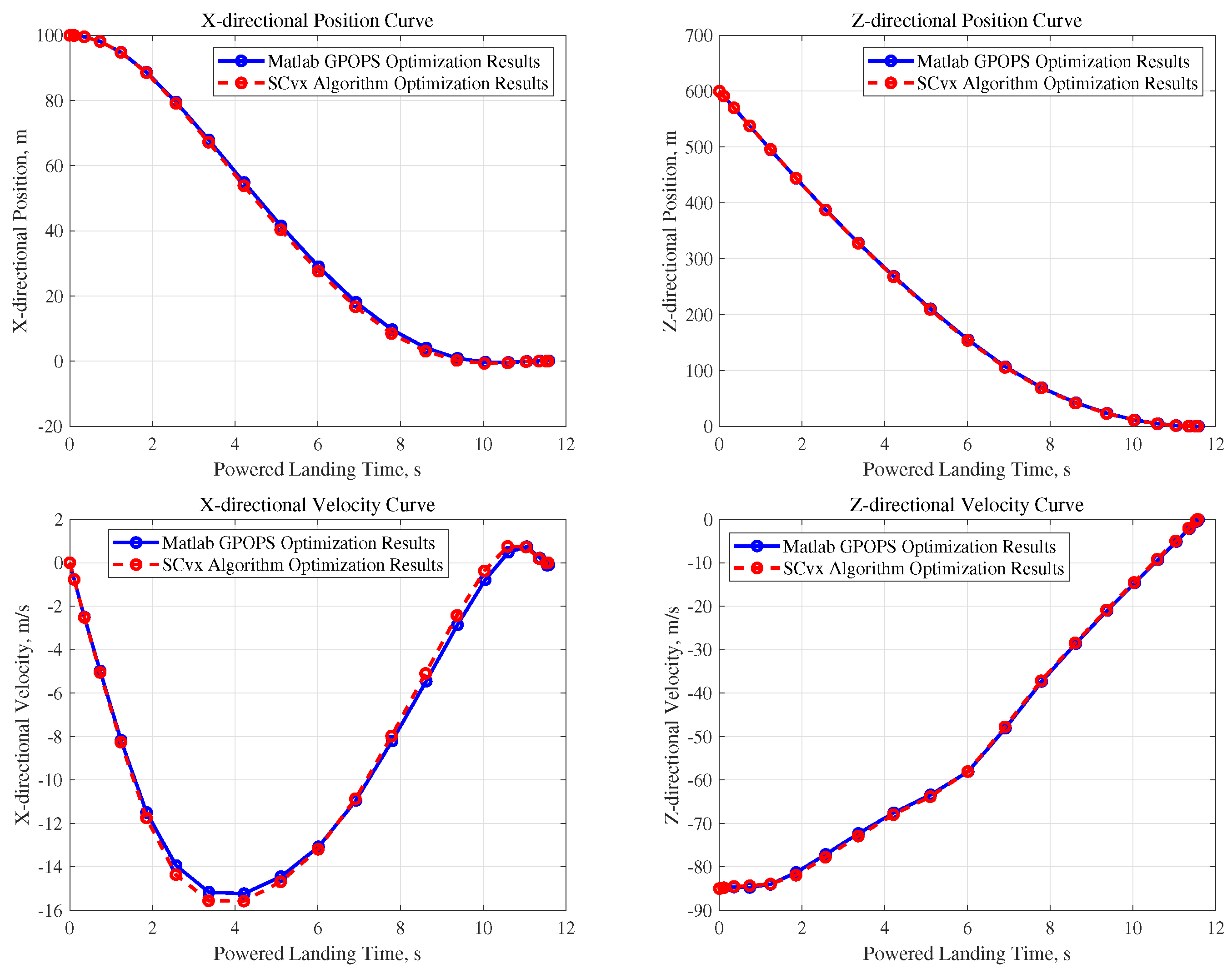
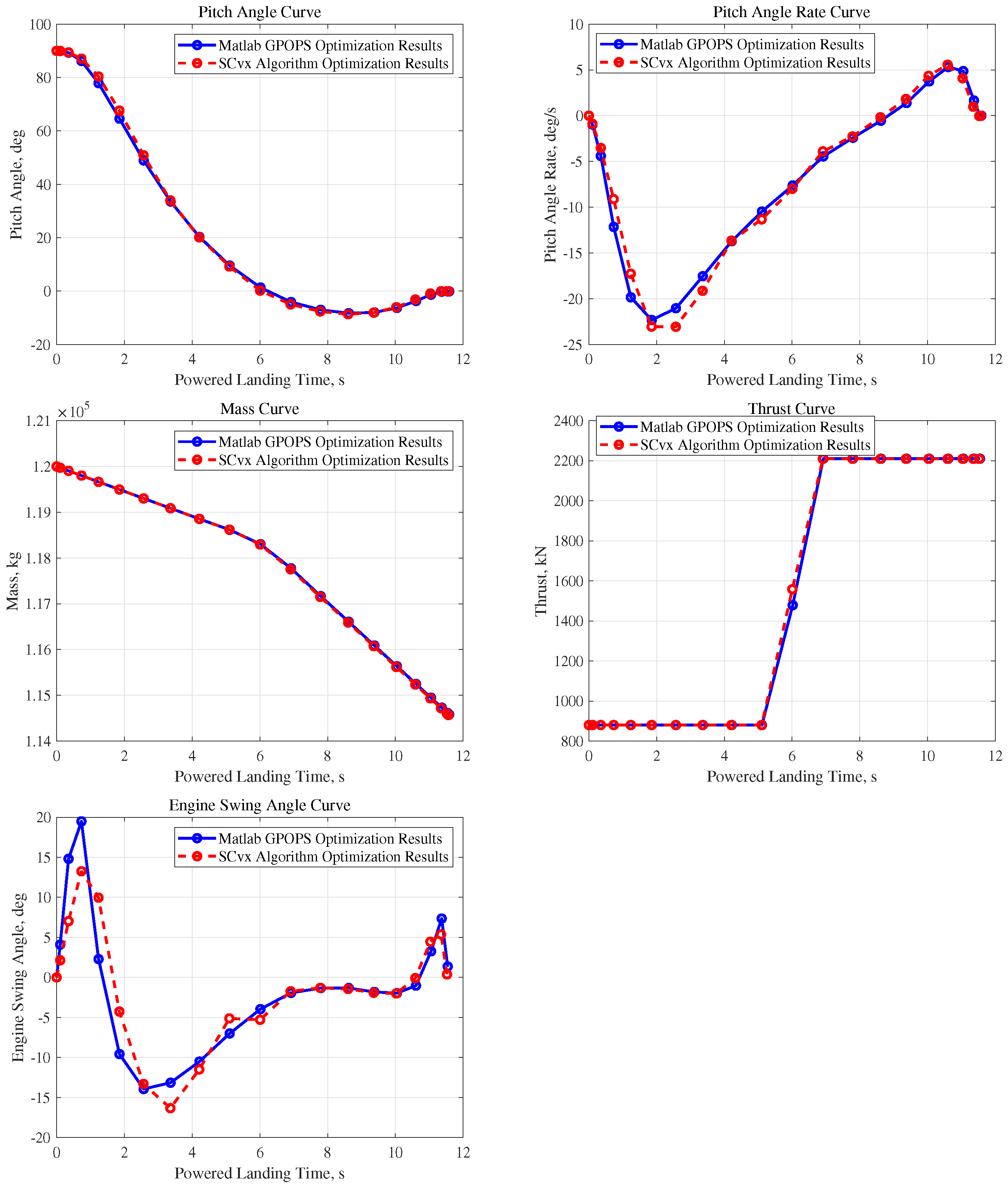
4.2. Hardware in the Loop Simulation Analysis

In this subsection, the performance of the proposed SCvx algorithm is verified by a hardware-in-the-loop simulation. The hardware-in-the-loop simulation system built based on the Speedgoat real-time target computer also includes the real-time simulation host computer, the onboard flight control computer, the simulated onboard guidance computer and the nozzle actuation simulator, and the main equipment components, etc, in which the GNC computers are analogous to those onboard the vehicle or at ground stations, the navigation computer collects the current vehicle status, the guidance computer runs the guidance algorithm and generates guidance commands based on the current vehicle status, and the control computer generates control commands based on the guidance information. The system architecture is shown in Figure 3. The test experiment uses a self-developed dedicated guidance and control computer, which is based on the NVIDIA Jetson Xavier NX motherboard as the core computing unit, the operating system is Ubuntu 18.04.5 LTS, the Visual Studio Code integrated development environment, using standard C programming language, the CPU is NVIDIA Carmel Arm v8.2 64-bit CPU with 1.4 GHz, 6 cores and 16 GB RAM.

This subsection compares the SCvx algorithm proposed in this paper with the Matlab GPOPS-II package, a RPM package that has been tested in a wide range of problem solving and is a typical representative of software based on pseudospectral method and nonlinear programming. Therefore, GPOPS-II is used in this paper to verify the correctness of the algorithm. In this calculation example, the number of collocation points are set to 20. The convex optimization procedure formed by the SCvx algorithm through C programming uses the trajectory generated by linear interpolation after concatenating the initial and terminal points as the initial trajectory, which is solved by the IPM solver ECOS.

From the results in Figure 4 and

Table 3. Optimization results.

Optimization Procedure	Terminal Moment	Terminal Mass	CPU Time Consumption
SCvx Algorithm	11.5666 s	114,568.6 kg	0.286 s
Matlab GPOPS	11.5666 s	114,580.7 kg	∕

, it can be seen that the results obtained from the optimization of the SCvx algorithm procedure are in basic agreement with Matlab GPOPS-II. In terms of computational speed, the computational time consumed by the SCvx algorithm procedure is 0.286 s, which satisfies the requirement of computational efficiency for online trajectory optimization for powered landing. The number of iterations at the end of the SCvx algorithm procedure is 5, which indicates that the proposed SCvx algorithm can obtain the optimal solution by iteration without exact initial values. The large attitude flip planar landing trajectory of the SLV is shown in Figure 5, which can more visually reflect the vertical landing process of the vehicle under the SCvx guidance algorithm.

The landing precision of the optimization results of the SCvx algorithm and Matlab GPOPS-II are shown in

Table 4. Comparison of SCvx algorithm and Matlab GPOPS-II integration precision.

Optimization Procedure	Positional Precision	Velocity Precision
SCvx Algorithm	0.77127 m	0.30135 m/s
Matlab GPOPS	0.62173 m	0.33001 m/s

. The two are comparable in magnitude, and the precision differs for different simulation conditions (e.g., number of discretization points, see

Table 5. Precision Comparison with Different Number of Collocation Points.

Optimization Procedure	Number of Collocation Points	Positional Precision	Velocity Precision
SCvx Algorithm	15	1.1597 m	0.29861 m/s
	20	0.77127 m	0.30135 m/s
	30	0.7097 m	0.23689m/s
Matlab GPOPS	15	1.1636m	0.39594 m/s
	20	0.62173 m	0.33001 m/s
	30	0.42617 m	0.1531 m/s

), i.e., the SCvx algorithm proposed in this paper achieves the precision of a general RPM-based nonlinear programming algorithm. When the number of discretization points increases, the landing precision also increases, but the computational efficiency decreases. By comparing the above optimization results, the correctness of the SCvx algorithm can be verified. Meanwhile, the advantage of the SCvx algorithm in computational efficiency makes it possible for onboard operation.

5. Conclusions

For the online trajectory optimization problem of LAFVL problem of SLV, a SCvx algorithm combining RPM and convex optimization techniques is proposed, which has high optimization precision and fast solving speed without exact initial values. The main research work and conclusions obtained in this paper are as follows. (1) The problem is discretized by the RPM with high precision, and the unique time-domain mapping of the RPM is used to transform the powered soft-landing terminal moments into special control variables, which is different from the fixed terminal moments method used in similar literature, and improves the optimization precision and optimality of the trajectory optimization results. (2) The nonconvex optimization model was convexified by combining LCvx and SCvx techniques to obtain a sequential convex optimization problem equivalent to the original problem. (3) The proposed SCvx algorithm is experimentally verified by a hardware-in-the-loop simulation platform to verify the correctness, high precision and fast convergence of the algorithm. In the future, we will further investigate the online guidance problem of the 6DOF dynamics model of SLV and design solution algorithms with faster computational efficiency in specific problems with more optimization variables and larger dimensionality.

References

1. Chen, S.Q.; Huang, H.; Shao, Y.T.; Huang, B. Study on the requirement trend and development suggestion for China space propulsion system. Astronaut. Syst. Eng. Technol. 2019, 3, 62–70. [Google Scholar]
2. Chen, S.Q.; Huang, H.; Zhang, Q.S.; Qin, X.D.; Rong, Y. Research on the development directions of Chinese launch vehicle liquid propulsion system. Astronaut. Syst. Eng. Technol. 2020, 4, 1–12. [Google Scholar]
3. Luo, M.; Chen, S.Q.; Li, D.P.; Pan, H. Characteristics of starship propulsion system and numerical simulation of propellant flow during reentry. J. Nanjing Univ. Aeronaut. Astronaut. 2021, 53, 9–16. [Google Scholar]
4. Song, Z.Y.; Wang, C. Development of online trajectory planning technology for launch vehicle return and landing. Astronaut. Syst. Eng. Technol. 2019, 3, 1–12. [Google Scholar]
5. Chen, Z.H.; Ning, L.; Wang, P. The development of launch vehicle booster recovery technology. Astronaut. Syst. Eng. Technol. 2021, 5, 66–74. [Google Scholar]
6. Hu, D.S.; Liu, N.; Liu, B.L.; Yan, N. Analysis on the development of reusable launch vehicles in the United States. Space Int. 2020, 12, 38–45. [Google Scholar]
7. Yang, K.; Mi, X. Analysis of the development of SpaceX’s reusable launch vehicle. Space Int. 2020, 9, 13–17. [Google Scholar]
8. Yan, N.; Hu, D.S.; Hao, Y.X. Analysis of SpaceX’s “Super HeavyStarship” transportation system scheme. Space Int. 2020, 11, 11–17. [Google Scholar]
9. Long, X.D. A brief analysis of the super-heavy-starship transport system and its future impact. Aerosp. Technol. 2021, 8, 32–35. [Google Scholar]
10. Cantou, T.; Merlinge, N.; Wuilbercq, R. 3DoF simulation model and specific aerodynamic control capabilities for a SpaceX’s Starship-like atmospheric reentry vehicle. In Proceedings of the 8nd European Conference for Aeronautics and Space Sciences, Madrid, Spain, 1–5 July 2019. [Google Scholar]
11. Palmer, C. SpaceX starship lands on Earth, But manned missions to Mars will require more. Engineering 2021, 7, 1345–1347. [Google Scholar] [CrossRef]
12. Liu, X. Autonomous Trajectory Planning by Convex Optimization; Iowa State University: Ames, IA, USA, 2013. [Google Scholar]
13. Liu, X.; Lu, P.; Pan, B. Survey of convex optimization for aerospace applications. Astrodynamics 2017, 1, 23–40. [Google Scholar] [CrossRef]
14. Açıkmeşe, B.; Blackmore, L. Lossless convexification of a class of optimal control problems with non-convex control constraints. Automatica 2011, 47, 341–347. [Google Scholar] [CrossRef]
15. Blackmore, L.; Açıkmeşe, B.; Carson, J.M. Lossless convexification of control constraints for a class of nonlinear optimal control problems. Syst. Control. Lett. 2012, 61, 863–870. [Google Scholar] [CrossRef]
16. Harris, M.W.; Açıkmeşe, B. Lossless convexification of non-convex optimal control problems for state constrained linear systems. Automatica 2014, 50, 2304–2311. [Google Scholar] [CrossRef]
17. Acikmese, B.; Ploen, S.R. Convex programming approach to powered descent guidance for mars landing. J. Guid. Control Dyn. 2007, 30, 1353–1366. [Google Scholar] [CrossRef]
18. Cheng, X.; Li, H.; Zhang, R. Efficient ascent trajectory optimization using convex models based on the Newton–Kantorovich/Pseudospectral approach. Aerosp. Sci. Technol. 2017, 66, 140–151. [Google Scholar] [CrossRef]
19. Zhang, K.; Yang, S.; Xiong, F. Rapid ascent trajectory optimization for guided rockets via sequential convex programming. Proc. Inst. Mech. Eng. Part G J. Aerosp. Eng. 2019, 233, 4800–4809. [Google Scholar] [CrossRef]
20. Zhang, Z.; Li, J.; Wang, J. Sequential convex programming for nonlinear optimal control problems in UAV path planning. Aerosp. Sci. Technol. 2018, 76, 280–290. [Google Scholar] [CrossRef]
21. Reynolds, T.P. Computational Guidance and Control for Aerospace Systems; University of Washington: Seattle, WA, USA, 2020. [Google Scholar]
22. Malyuta, D. Convex Optimization in a Nonconvex World: Applications for Aerospace Systems; University of Washington: Seattle, WA, USA, 2021. [Google Scholar]
23. Garg, D. Advances in Global Pseudospectral Methods for Optimal Control; Massachusetts Institute of Technology: Cambridge, MA, USA, 2011. [Google Scholar]
24. Darby, C.L. hp-Pseudospectral Method for Solving Continuous-Time Nonlinear Optimal Control Problems; University of Florida: Gainesville, FL, USA, 2011. [Google Scholar]
25. Wang, J.B.; Cui, N.G.; Guo, J.F.; Xu, D.F. High precision rapid trajectory optimization algorithm for launch vehicle landing. Control Theory Appl. 2018, 35, 389–398. [Google Scholar]
26. Wang, J.B.; Cui, N.G. A pseudospectral-convex optimization algorithm for rocket landing guidance. In Proceedings of the 2018 AIAA Guidance, Navigation, and Control Conference, Kissimmee, FL, USA, 8–12 January 2018; p. 1871. [Google Scholar]
27. Szmuk, M.; Pascucci, C.A.; Dueri, D. Convexification and real-time on-board optimization for agile quad-rotor maneuvering and obstacle avoidance. In Proceedings of the 2017 IEEE/RSJ International Conference on Intelligent Robots and Systems (IROS), Vancouver, BC, Canada, 24–28 September 2017; pp. 4862–4868. [Google Scholar]
28. Zhou, D.; Zhang, Y.; Li, S. Receding horizon guidance and control using sequential convex programming for spacecraft 6-DOF close proximity. Aerosp. Sci. Technol. 2019, 87, 459–477. [Google Scholar] [CrossRef]
29. Wang, Z.B. Optimal trajectories and normal load analysis of hypersonic glide vehicles via convex optimization. Aerosp. Sci. Technol. 2019, 87, 357–368. [Google Scholar] [CrossRef]
30. Wang, J.B.; Ma, H.J.; Li, H.X.; Chen, H.B. Real-time guidance for powered landing of reusable rockets via deep learning. Neural Comput. Appl. 2022, 1–22. [Google Scholar] [CrossRef]
31. Furfaro, R.; Scorsoglio, A.; Linares, R. Adaptive generalized ZEM-ZEV feedback guidance for planetary landing via a deep reinforcement learning approach. Acta Astronaut. 2020, 171, 156–171. [Google Scholar] [CrossRef]
32. Gaudet, B.; Linares, R.; Furfaro, R. Deep reinforcement learning for six degree-of-freedom planetary landing. Adv. Space Res. 2020, 65, 1723–1741. [Google Scholar] [CrossRef]
33. Xu, X.; Chen, Y.; Bai, C. Deep Reinforcement Learning-Based Accurate Control of Planetary Soft Landing. Sensors 2021, 21, 8161. [Google Scholar] [CrossRef]
34. Dueri, D.; Açıkmeşe, B.; Scharf, D.P.; Harris, M.W. Customized real-time interior-point methods for onboard powered-descent guidance. J. Guid. Control Dyn. 2017, 40, 197–212. [Google Scholar] [CrossRef]
35. Dueri, D.; Zhang, J.; Açikmese, B. Automated custom code generation for embedded, real-time second order cone programming. IFAC Proc. Vol. 2014, 47, 1605–1612. [Google Scholar] [CrossRef]
36. Ren, G.F.; Gao, A.; Cui, P.Y.; Luan, E.J. A rapid power descent phase trajectory optimization method with minimum fuel consumption for Mars pinpoint landing. J. Astronaut. 2014, 35, 1350–1358. [Google Scholar]
Figure 1. Planar landing model considering pitch attitude motion.
Mathematics 11 00288 g001
Figure 2. Comparison of optimization results for P 1 , P 2 and P 3 .
Mathematics 11 00288 g002
Figure 3. Hardware-in-the-loop simulation system framework.
Mathematics 11 00288 g003
Figure 4. Comparison of optimization trajectories.
Mathematics 11 00288 g004aMathematics 11 00288 g004b
Figure 5. Starship large attitude flip planar landing trajectory.
Mathematics 11 00288 g005