Zero-Dependent Bivariate Poisson Distribution with Applications

Abstract

The bivariate Poisson model is the most widely used model for bivariate counts, and in recent years, several bivariate Poisson regression models have been developed in order to analyse two response variables that are possibly correlated. In this paper, a particular class of bivariate Poisson model, developed from the bivariate Bernoulli model, will be presented and investigated. The proposed bivariate Poisson models use dependence parameters that can model positively and negatively correlated data, whereas more well-known models, such as Holgate’s bivariate Poisson model, can only be used for positively correlated data. As a result, the proposed model contributes to improving the properties of the more common bivariate Poisson regression models. Furthermore, some of the properties of the new bivariate Poisson model are outlined. The method of maximum likelihood and moment method were used to estimate the parameters of the proposed model. Additionally, real data from the healthcare utilization sector were used. As in the case of healthcare utilization, dependence between the two variables may be positive or negative in order to assess the performance of the proposed model, in comparison to traditional bivariate count models. All computations and graphs shown in this paper were produced using R programming language.

1. Introduction

Bivariate count models have received increasing scholarly attention in recent years, mainly because they offer flexibility for fitting across a wide variety of random phenomena. For instance, applications based on discrete bivariate models are often used in the fields of health sciences, traffic accidents, economics, actuarial science, social sciences, environmental studies, and so forth [1]. For more information about bivariate count models, the reader is directed to [2,3,4,5,6,7,8]. The most widely used model for bivariate counts is the bivariate Poisson model, which was developed by [9]. The bivariate Poisson model, which was developed by [9], is considered the limit of a bivariate contingency table model. The literature outlines the main contributions and applications of bivariate Poisson models. For instance, the bivariate Poisson model can be used in modelling data in sports [10,11], health [12,13,14], econometrics and insurance [15,16], and so forth. Furthermore, the use of the bivariate Poisson model is not unique in its different methodological applications. One of the methods is the trivariate reduction, which was studied by [17] and developed by [18]. Bivariate Poisson models have been developed based on the method of trivariate reduction using convolutions of independent Poisson random variables. These models allow for only non-negative correlation between variables. For a comprehensive review of the bivariate Poisson model and its applications, the reader is directed to references [4,19,20,21].

More recently, researchers have developed bivariate Poisson regression models. These models analyse two response variables that are possibly correlated, and they allow the two response variables to be affected by different predictive factors. This means that bivariate Poisson regression models can be used for inference and prediction purposes. Early studies of the use of bivariate count regression models to analyse correlated count events include those by [3], who use a bivariate Poisson regression in a labour mobility study. Furthermore, using a bivariate Poisson regression model, [22] study the relationship between types of health insurance and various responses that measure the demand for health care. Only recently have bivariate regression models been compared and their application in different fields analysed in depth. A study by [13] examines bivariate and zero-inflated bivariate Poisson regression models using the conditional method, as compared with the standard method, using a joint probability distribution (j.p.d). Therefore, bivariate Poisson regression models play a vital role in modeling, analyzing, and improving the fit results when two dependent variables in a data set are highly correlated [1,12,23].

Although the bivariate Poisson regression model offers useful properties for modeling paired count data that exhibits correlations, some models have major drawbacks. One drawback is that some models can only model data with positive correlations [24]. For instance, a bivariate Poisson model based on the trivariate reduction method studied by [17] lacks generality, because it shows a positive correlation only. A few previous studies have explored and developed bivariate Poisson regression models that allow for negative correlations, including bivariate Poisson distribution as a product of Poisson marginals with a multiplicative factor [5]. In addition, [25] have proposed a bivariate Poisson distribution that allows for negative correlations by using conditional probabilities. This current paper will consider a class of bivariate Poisson models generated from the bivariate Bernoulli model, which can model positively and negatively correlated data. This is a progression on from other bivariate Poisson models already proposed in previous research, including the well-known Holgate [17] bivariate Poisson model. One of the merits of the proposed model is that its structure is relatively simple. The proposed models seek to contribute to improving the properties of commonly used bivariate Poisson models. In this paper, the statistical properties of the new model are studied, and the parameters of the proposed model are estimated using the maximum likelihood and moment methods. In this respect, a simulation study was carried out to investigate the performance of the parameter estimation ability of the proposed model using the maximum likelihood and moment method. Finally, applications of the proposed model will be presented in the healthcare sector, and the model’s performance will be compared against well-known bivariate Poisson models.

This paper is organized into sections as follows: Section 2 will detail the proposed bivariate Poisson model and the relevant estimation methods used. Section 3 will present relevant application of this model, using data drawn from different fields and will compare the results with well-known models. Finally, a conclusion will be presented in Section 4.

2. Zero-Dependent Bivariate Poisson Model (ZDBP)

Different methods have been used to construct bivariate Poisson distributions, with specified marginal distributions. Most of the well-known bivariate Poisson models use the popular reduction method [4]. However, this method has two main drawbacks. Firstly, it does not support negative correlation values and secondly, it does not cover the entire range of feasible correlations. In the current study, the construction of a developed bivariate Poisson model is presented, without the aforementioned drawbacks as follows:

If we consider that $(B_1, B_2)$ has Bernoulli marginals, then it has only four possible values $\left(1, 1\right)$, $\left(1, 0\right)$, $\left(0, 1\right),$ and $\left(0, 0\right)$ with the probabilities $p_{11}$, $p_{10}$, $p_{01},$ and $p_{00,}$ which are $p_{ij}=P\left(B_1=i, B_2=j\right), i,j=0,1$. If the marginal probability discrete random variables are independent of $\left(B_1,B_2\right)$, and have a probability mass function of zero-truncated Poisson distribution with the parameters ${\theta }_1$ and ${\theta }_2,$ respectively, then the probability mass function can be defined as follows:

$$P(X_i=j)=\frac{e^{-{\theta }_i}}{1-e^{-{\theta }_i}}\frac{{\theta }_i{}^j}{j!}, j=1,2,\dots , i=1,2$$

.

Here, set $Y_i=B_i{X}_i, i=1,2,$ where $p_i=1-e^{-{\theta }_i}, i=1,2$. Then, $Y_i$ has a Poisson distribution with the parameter ${\theta }_i$. The j.d.f of the two random variables, $Y_1$ and $Y_2,$ can be expressed as follows:

$$P(Y_1=y_1, Y_2=y_2)={\displaystyle \sum }_{i,j=0}^{1}P(Y_1=y_1, Y_2=y_2|B_1=i, B_2=j)p_{ij}$$

Then:

$$\begin{array}{ll}P(Y_1=y_1, Y_2=y_2)& \\ =\frac{{\theta }_1{}^{y_1}}{y_1!}\frac{{\theta }_2{}^{y_2}}{y_2!}{\left(\frac{1-p_1}{p_1}\right)}^{1-\delta \left(y_1\right)}{\left(\frac{1-p_2}{p_2}\right)}^{1-\delta \left(y_2\right)} p_{00}{}^{\delta \left(y_1\right)\delta \left(y_2\right)}{p}_{10}{}^{\left(1-\delta \left(y_1\right)\right)\delta \left(y_2\right)}{p}_{01}{}^{\delta \left(y_1\right)\left(1-\delta \left(y_2\right)\right)}{p}_{11}{}^{\left(1-\delta \left(y_1\right)\right)\left(1-\delta \left(y_2\right)\right)}\end{array}$$

(1)

for $y_1,y_2=0,1,\dots$ where $\delta \left(x\right)=1$ if $x=0$ and $0$ is otherwise.

Generally, $Y_1$ and $Y_2$ are dependent and therefore (1) defines a new bivariate Poisson distribution, which will be called the zero-dependent Bivariate Poisson Model (ZDBP) model. Since bivariate Bernoulli distribution is completely determined by the three parameters $p_1, p_2$, and $p_{11},$ then, the above shows that the ZDBP model is completely determined by the three parameters ${\theta }_1,{\theta }_2$, and $p_{11}$. Therefore, the ZDBP (${\theta }_1,{\theta }_2, p_{11})$ model can be used whenever the parameters matter and as a result, (1) can be rewritten as follows:

$$\begin{array}{ll}P(Y_1=y_1, Y_2=y_2)& \\ & =\frac{{\theta }_1{}^{y_1}}{y_1!}\frac{{\theta }_2{}^{y_2}}{y_2!}{\left(\frac{e^{-{\theta }_1}}{1-e^{-{\theta }_1}}\right)}^{1-\delta \left(y_1\right)}{\left(\frac{e^{-{\theta }_2}}{1-e^{-{\theta }_2}}\right)}^{1-\delta \left(y_2\right)} {\left(e^{-{\theta }_1}+e^{-{\theta }_2}+p_{11}-1\right)}^{\delta \left(y_1\right)\delta \left(y_2\right)} (1-e^{-{\theta }_1}\\ & -p_{11}{)}^{\delta \left(y_2\right)\left(1-\delta \left(y_1\right)\right)} {\left(1-e^{-{\theta }_2}-p_{11}\right)}^{\delta \left(y_1\right)\left(1-\delta \left(y_2\right)\right)}{p}_{11}{}^{\left(1-\delta \left(y_1\right)\right)\left(1-\delta \left(y_2\right)\right)}\end{array}$$

(2)

To visualize the j.p.d for the ZDBP model in (2), the representative j.p.d plots for different parameter choices are shown in Figure 1, Figure 2 and Figure 3, where negative dependence is apparent in Figure 1 and Figure 3. The package “plot3D” in R is needed to represent the plots in Figure 1, Figure 2 and Figure 3.

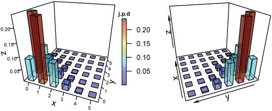
Figure 1. The j.p.d of the ZDBP model for ${\theta }_1=0.79,{\theta }_2=0.79$ and $p_{11}=0.19$ with $cor=-0.3$.

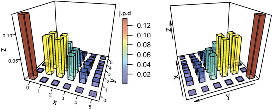
Figure 2. The j.p.d of the ZDBP model for ${\theta }_1=1.96,{\theta }_2=1.96$ and $p_{11}=0.85$ with $cor=0.3$.

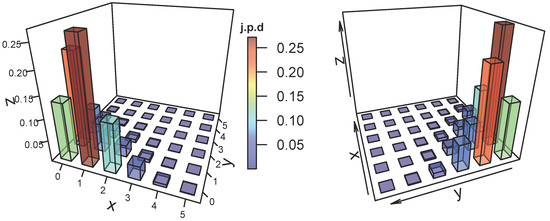
Figure 3. The j.p.d of the ZDBP model for ${\theta }_1=0.84,{\theta }_2=0.58$ and $p_{11}=0.15$ with $cor=-0.3$.

2.1. Statistical Properties

The ZDBP model has statistical properties that can be easily proven. These properties are shown as follows:

Theorem 1.

The conditional probability function of $Y_1$given$Y_2$is

$$P(Y_1=y_1| Y_2=y_2)=\left\{\begin{array}{c} P_0\left(y_2\right) y_1=0 \\ (1-P_0\left(y_2\right))\frac{{\theta }_1{}^{y_1}}{y_1!}\left(\frac{e^{-{\theta }_1}}{1-e^{-{\theta }_1}}\right) y_1=1,2,\dots \end{array}\right. ,$$

where,

$$P_0\left(y_2\right)=e^{{\theta }_2}{\left(\frac{e^{-{\theta }_2}}{1-e^{-{\theta }_2}}\right)}^{1-\delta \left(y_2\right)} {\left(e^{-{\theta }_1}+e^{-{\theta }_2}+p_{11}-1\right)}^{\delta \left(y_2\right)} {\left(1-e^{-{\theta }_2}-p_{11}\right)}^{\left(1-\delta \left(y_2\right)\right)}$$

Proof .

Dividing (2) by $\frac{{\theta }_2{}^{y_2}}{y_2!}{e}^{-{\theta }_2}$ one gets

$$P(Y_1=y_1| Y_2=y_2)=e^{{\theta }_2}\frac{{\theta }_1{}^{y_1}}{y_1!}{\left(\frac{e^{-{\theta }_1}}{1-e^{-{\theta }_1}}\right)}^{1-\delta \left(y_1\right)}{\left(\frac{e^{-{\theta }_2}}{1-e^{-{\theta }_2}}\right)}^{1-\delta \left(y_2\right)} {\left(e^{-{\theta }_1}+e^{-{\theta }_2}+p_{11}-1\right)}^{\delta \left(y_1\right)\delta \left(y_2\right)}$$

$${\left(1-e^{-{\theta }_1}-p_{11}\right)}^{\delta \left(y_2\right)\left(1-\delta \left(y_1\right)\right)} {\left(1-e^{-{\theta }_2}-p_{11}\right)}^{\delta \left(y_1\right)\left(1-\delta \left(y_2\right)\right)}{p}_{11}{}^{\left(1-\delta \left(y_1\right)\right)\left(1-\delta \left(y_2\right)\right)}.$$

Therefore, for $y_1=0,$ we have

$$P(Y_1=0| Y_2=y_2)=e^{{\theta }_2}{\left(\frac{e^{-{\theta }_2}}{1-e^{-{\theta }_2}}\right)}^{1-\delta \left(y_2\right)} {\left(e^{-{\theta }_1}+e^{-{\theta }_2}+p_{11}-1\right)}^{\delta \left(y_2\right)} {\left(1-e^{-{\theta }_2}-p_{11}\right)}^{\left(1-\delta \left(y_2\right)\right)}=P_0\left(y_2\right).$$

In addition, for $y_1\ne 0$, we have

$$P(Y_1=y_1| Y_2=y_2)=e^{{\theta }_2}\frac{{\theta }_1{}^{y_1}}{y_1!}\left(\frac{e^{-{\theta }_1}}{1-e^{-{\theta }_1}}\right){\left(\frac{e^{-{\theta }_2}}{1-e^{-{\theta }_2}}\right)}^{1-\delta \left(y_2\right)} {\left(1-e^{-{\theta }_1}-p_{11}\right)}^{\delta \left(y_2\right)}{p}_{11}{}^{\left(1-\delta \left(y_2\right)\right)}$$

From the two cases $y_2=0$ and $y_2\ne 0$, we conclude that

$$e^{{\theta }_2}{\left(\frac{e^{-{\theta }_2}}{1-e^{-{\theta }_2}}\right)}^{1-\delta \left(y_2\right)} \left[{\left(e^{-{\theta }_1}+e^{-{\theta }_2}+p_{11}-1\right)}^{\delta \left(y_2\right)} {\left(1-e^{-{\theta }_2}-p_{11}\right)}^{\left(1-\delta \left(y_2\right)\right)}+e^{{\theta }_2}\frac{{\theta }_1{}^{y_1}}{y_1!} {\left(1-e^{-{\theta }_1}-p_{11}\right)}^{\delta \left(y_2\right)}{p}_{11}{}^{\left(1-\delta \left(y_2\right)\right)}\right]=1,$$

As a result, we get

$$e^{{\theta }_2}{\left(\frac{e^{-{\theta }_2}}{1-e^{-{\theta }_2}}\right)}^{1-\delta \left(y_2\right)} {\left(1-e^{-{\theta }_1}-p_{11}\right)}^{\delta \left(y_2\right)}{p}_{11}{}^{\left(1-\delta \left(y_2\right)\right)}=1-P_0\left(y_2\right).$$

This completes the proof. □

From the above, it is clear that Theorem 1 implies that the conditional distribution of $Y_1$ given $Y_2$ is mixture of degenerated distribution at zero and zero-truncated Poisson distribution with mixing probabilities dependent on the value of $y_2$. In other words, we can write $Y_1|Y_2{=}^{d}I\left(Y_2\right)R,$ where $I\left(Y_2\right)$ is the Bernoulli random variable with failure probability as $P_0\left(Y_2\right)$ independent of the zero-truncated Poisson random variable $R$. Therefore, we have the following corollary.

Corollary 1.

$$E\left[Y_1|Y_2=y_2\right]=\frac{{\theta }_1}{1-e^{-{\theta }_1}}\left[1-P_0\left(y_2\right)\right]=\frac{{\theta }_1}{1-e^{-{\theta }_1}}\left\{\begin{array}{c}{e}^{{\theta }_2}\left(1-e^{-{\theta }_1}-p_{11}\right), y_2=0 \\ \frac{p_{11}}{1-e^{-{\theta }_2}} , y_2\ne 0\end{array}\right.$$

Theorem 2.

The covariance of$Y_1$and$Y_2$is$cov\left(Y_1,Y_2\right)=\frac{{\theta }_1{\theta }_2}{p_1{p}_2}\left(p_{11}-p_1{p}_2\right)$

Proof .

The covariance of $Y_1$ and $Y_2$ according to the assumption $Y_i=B_i{X}_i, i=1,2$ can be defined as follows:

$$cov\left(Y_1,Y_2\right)=cov\left(B_1{X}_1,B_2{X}_2\right)=E\left(B_1{X}_1{B}_2{X}_2\right)-E\left(B_1{X}_1\right)E\left(B_2{X}_2\right)$$

Since $X_1$ and $X_2$ are independent of $\left(B_1,B_2\right)$, then

$$\begin{gathered} cov\left(Y_1,Y_2\right)=E\left(X_1\right)E\left(X_2\right)E\left(B_1{B}_2\right)-E\left(X_1\right)E\left(X_2\right)E\left(B_1\right)E\left(B_2\right)= \mathrm{E}\left(X_1\right)\mathrm{E}\left(X_2\right)\left[\mathrm{E}\left(B_1{B}_2\right)- \mathrm{E}\left(B_1\right)\mathrm{E}\left(B_2\right)\right] \\ =\frac{{\theta }_1{\theta }_2}{\left(1-e^{-{\theta }_1}\right)\left(1-e^{-{\theta }_2}\right)}cov\left(B_1,B_2\right) \end{gathered}$$

Since $cov\left(B_1,B_2\right)=p_{11}-p_1{p}_2$ and $p_i=1-e^{-{\theta }_i},$ therefore we get the result

$$cov\left(Y_1,Y_2\right)=\frac{{\theta }_1{\theta }_2}{p_1{p}_2}\left(p_{11}-p_1{p}_2\right)$$

□

From Corollary 1, it is clear that $Y_1$ and $Y_2$ will be independent variables when $p_{11}=p_1{p}_2$.

Corollary 2.

The correlation of$Y_1$and$Y_2$is$cor\left(Y_1,Y_2\right)=\sqrt{\frac{{\theta }_1{\theta }_2\left(1-p_1\right)\left(1-p_2\right)}{p_1{p}_2}}cor\left(B_1,B_2\right) .$

Proof .

The correlation of $Y_1$ and $Y_2$ according to the assumption $Y_i=B_i{X}_i, i=1,2$ is defined as follows:

$$cor\left(Y_1,Y_2\right)=cor\left(B_1{X}_1,B_2{X}_2\right)=\frac{cov\left(Y_1,Y_2\right)}{\sigma \left(Y_1\right)\sigma \left(Y_2\right)}$$

From Corollary 1 and since $Y_i~Poisson\left({\theta }_i\right), i=1,2,$ then

$$cor\left(Y_1,Y_2\right)=\frac{\sqrt{{\theta }_1{\theta }_2}}{p_1{p}_2}\left(p_{11}-p_1{p}_2\right)$$

Since $cor\left(B_1,B_2\right)=\frac{p_{11}-p_1{p}_2}{\sqrt{p_1\left(1-p_1\right)p_2\left(1-p_2\right)}}$, then the equation above can be written as

$$cor\left(Y_1,Y_2\right)=\sqrt{\frac{{\theta }_1{\theta }_2\left(1-p_1\right)\left(1-p_2\right)}{p_1{p}_2}}cor\left(B_1,B_2\right)$$

□

From Corollary 2, we can conclude that the correlation of $Y_1$ and $Y_2$ allows the ZDBP model to be positively or negatively correlated since it depends on $cor\left(B_1,B_2\right),$ which can be a negative or a positive correlation.

2.2. Parameter Estimation

An estimation of the ZDBP model parameters was obtained using the maximum likelihood estimation (ML) and moment methods (MM). The ZDBP model has six parameters that can be estimated based on three parameters, which are ${\theta }_1,{\theta }_2,$ and $p_{11}.$ If we consider $n$ as the independent vectors $\left(y_{i1},y_{i2}\right)$, where the $i$-th vector is the ZDBP model shown in (2), then the estimators can be expressed as follows:

2.2.1. Maximum Likelihood Estimation (ML)

The likelihood function of (2) is shown below as

$$\begin{array}{lll}L({\theta }_1,{\theta }_2,p_{11},p_{00},& p_{10},p_{01},p_{11};y_{1i},y_{2i})& \\ & =\prod _{i=1}^n\frac{{{\theta }_1}^{y_{1i}}}{y_{1i}!}\frac{{{\theta }_2}^{y_{2i}}}{y_{2i}!}{\left(\frac{e^{-{\theta }_1}}{1-e^{-{\theta }_1}}\right)}^{1-\delta \left(y_{1i}\right)}{\left(\frac{e^{-{\theta }_2}}{1-e^{-{\theta }_2}}\right)}^{1-\delta \left(y_{2i}\right)}{(e^{-{\theta }_1}+e^{-{\theta }_2}+p_{11}-1)}^{\delta \left(y_{1i}\right)\delta \left(y_{2i}\right)}(1-e^{-{\theta }_1}\\ & -p_{11}{)}^{\delta \left(y_{2i}\right)\left(1-\delta \left(y_{1i}\right)\right)}{(1-e^{-{\theta }_2}-p_{11})}^{\delta \left(y_{1i}\right)\left(1-\delta \left(y_{2i}\right)\right)}{p_{11}}^{\left(1-\delta \left(y_{1i}\right)\right)\left(1-\delta \left(y_{2i}\right)\right)}\end{array}$$

It is worth mentioning that ${\theta }_1,{\theta }_2,$ and $p_{11}$ are sufficient to be used with ML method in order to estimate the other parameters. This is because of the dependent relationship between the parameters. The corresponding log likelihood can be given as follows:

$$\begin{array}{lll}\ell =logL({\theta }_1,{\theta }_2,& p_{11};y_{1i},y_{2i})& \\ & =\sum _{i=1}^n[y_{1i}\log \left({\theta }_1\right)-\log \left(y_{1i}!\right)+y_{2i}\log \left({\theta }_2\right)-\log \left(y_{2i}!\right)-\left(1-\delta \left(y_{1i}\right)\right)\left({\theta }_1+\log \left(1-e^{-{\theta }_1}\right)\right)\\ & -\left(1-\delta \left(y_{2i}\right)\right)\left({\theta }_2+\log \left(1-e^{-{\theta }_2}\right)\right)+\delta \left(y_{1i}\right)\delta \left(y_{2i}\right)\log (e^{-{\theta }_1}+e^{-{\theta }_2}+p_{11}-1)\\ & +\delta \left(y_{2i}\right)\left(1-\delta \left(y_{1i}\right)\right)log(1-e^{-{\theta }_1}-p_{11})+\delta \left(y_{1i}\right)\left(1-\delta \left(y_{2i}\right)\right)log(1-e^{-{\theta }_2}-p_{11})\\ & +\left(1-\delta \left(y_{1i}\right)\right)\left(1-\delta \left(y_{2i}\right)\right)\log \left(p_{11}\right)]\end{array}$$

Furthermore, the corresponding likelihood equations are shown below:

$$\frac{\partial \ell }{\partial {\widehat{\theta }}_1}=0,\frac{\partial \ell }{\partial {\widehat{\theta }}_2}=0 \mathrm{and} \frac{\partial \ell }{\partial {\widehat{p}}_{11}}=0$$

(3)

These equations can be solved numerically to estimate the parameters ${\theta }_1,{\theta }_2,$ and $p_{11}$. Following on from this, other parameters were estimated using the following equations:

$$\left.\begin{array}{c}{\widehat{p}}_1=1-e^{-{\widehat{\theta }}_1}\\ {\widehat{p}}_2=1-e^{-{\widehat{\theta }}_2}\\ {\widehat{p}}_{10}=1-e^{-{\widehat{\theta }}_1}-{\widehat{p}}_{11}\\ {\widehat{p}}_{01}=1-e^{-{\widehat{\theta }}_2}-{\widehat{p}}_{11}\\ {\widehat{p}}_{00}=e^{-{\widehat{\theta }}_1}+e^{-{\widehat{\theta }}_2}+{\widehat{p}}_{11}-1\end{array}\right\}$$

(4)

2.2.2. Moment Method Estimation (MM)

Using the MM, the following equations were considered in order to estimate the parameters ${\theta }_1,{\theta }_{2,}$ and $p_{11}$ as follows:

$$\left.\begin{array}{c}{\overline{y}}_1={\widehat{\theta }}_1\\ {\overline{y}}_2={\widehat{\theta }}_2\\ {\widehat{p}}_{11}=\left(1-e^{-{\widehat{\theta }}_1}\right)\left(1-e^{-{\widehat{\theta }}_2}\right)\left[\frac{\widehat{\gamma }}{{\widehat{\theta }}_1{\widehat{\theta }}_2}+1\right]\end{array}\right\}$$

Following on from this, other parameters were estimated using (4).

2.2.3. Simulation Study

A simulation study was conducted to assess the performance of the ML method and MM used for the estimation of ZDBP’s parameters. The simulation was executed according to the steps outlined below:

• A total of 1000 data sets with sizes of 20, 50, 200, and 1000, relating to each data set, were generated from the ZDBP model using four different theoretical parameters values, with varying positive and negative correlations as follows:

  (a)

  Case 1: Model ZDBP ($0.30,1.57, 0.05)$ with $cor=-$0.5;

  (b)

  Case 2: Model ZDBP ($0.54,0.89, 0.07)$ with $cor=-$0.5;

  (c)

  Case 3: Model ZDBP ($0.44,0.37, 0.19)$ with $cor=$ 0.3;

  (d)

  Case 4: Model ZDBP ($0.17,0.19, 0.13)$ with $cor=$ 0.7.

• Calculating the ML estimates of ${\theta }_1,{\theta }_2,$ and $p_{11}$ and considering that $1-e^{-{\widehat{\theta }}_1}-e^{-{\widehat{\theta }}_2}\le {\widehat{p}}_{11}\le \min \left\{1-e^{-{\widehat{\theta }}_1}, 1-e^{-{\widehat{\theta }}_2}\right\}$, the obtained estimates by step 1 were ignored.
• The bias and mean square error (MSE) were calculated for all considered models.

In Step 1, packages “mipfp”, “VGAM”, and “actuar” in R were used in order to generate data from the ZDBP model. In addition, in Step 2, Equation (3) is solved numerically using the function “optim” in R. The method “BFGS”, a quasi-Newton method, was chosen for the optimization problem among other methods in optim function because it is relatively quick. Table 1, Table 2, Table 3 and Table 4 below show the performance of the ML method and the MM used for estimation of the ZDBP’ parameters, taking into account the MSE and bias relating to the cases shown in Step 1 of the simulation study. In general, the results revealed the superiority of the ML method for the estimation of positive and negative correlations in comparison with the MM, taking into account the MSE. In addition, the ML results of ${\theta }_1,{\theta }_2,$ and $p_{11}$ were better than the MM results of these parameters based on the MSE for n = 20, except for the ML results of ${\theta }_1,{\theta }_2$, when ${\theta }_1>{\theta }_2,$ as shown in Table 1.

Table 1. MSE and bias between parentheses for the different simulated data sizes: n = 20, 50, 200, 1000 for the ZDBP ($0.30,1.57, 0.05)$ model with cor = −0.5.

n		20		50		200		1000
Method		ML	MM	ML	MM	ML	MM	ML	MM
${\widehat{\theta }}_1$	MSE	0.0038	0.0022	0.0101	0.0014	0.0002	0.0017	0.0002	0.0004
	bias	0.0467	0.0468	0.2867	0.0368	0.0092	0.0393	0.0087	0.0138
${\widehat{\theta }}_2$	MSE	0.1937	0.1092	0.0002	0.0271	0.0090	0.0096	0.0007	0.0004
	bias	−0.4347	−0.2630	−0.0138	0.1570	0.0948	0.0970	−0.0254	−0.0205
${\widehat{p}}_{11}$	MSE	0.0027	0.0047	0.0001	0.0001	0.0005	0.0006	0.0001	0.0001
	bias	−0.0329	−0.0600	0.0075	0.0010	0.0213	0.0204	0.0010	−0.0031
$\widehat{cor}$	MSE	0.0165	0.0682	0.0004	0.0088	0.0016	0.0010	0.0001	0.0007
	bias	−0.1118	−0.2447	0.0145	−0.0809	0.0397	−0.0034	−0.0032	−0.0257

Table 2. MSE and bias between parentheses for the different simulated data sizes: n = 20, 50, 200, 1000 for the ZDBP ($0.54,0.89, 0.07)$ model with cor = −0.5.

n		20		50		200		1000
Method		ML	MM	ML	MM	ML	MM	ML	MM
${\widehat{\theta }}_1$	MSE	0.0227	0.0251	0.0082	0.0097	0.0022	0.0027	0.0004	0.0005
	bias	−0.0048	0.0192	0.0026	0.0135	−0.0047	−0.0037	0.0001	0.0002
${\widehat{\theta }}_2$	MSE	0.0390	0.0415	0.0149	0.0162	0.0040	0.0043	0.0008	0.0009
	bias	−0.0061	0.0132	0.0012	0.0090	0.0006	0.0009	0.0005	0.0011
${\widehat{p}}_{11}$	MSE	0.0021	0.0040	0.0010	0.0017	0.0003	0.0005	0.0001	0.0001
	bias	−0.0155	−0.0163	0.0017	0.0018	−0.0003	0.0006	0.0005	0.0006
$\widehat{cor}$	MSE	0.0123	0.0290	0.0045	0.0100	0.0012	0.0027	0.0002	0.0005
	bias	−0.0600	−0.0900	−0.0048	−0.0164	0.0006	0.0021	0.0008	0.0007

Table 3. MSE and bias between parentheses for the different simulated data sizes: n = 20, 50, 200, 1000 for the ZDBP ($0.44,0.37, 0.19)$ model with cor = 0.3.

n		20		50		200		1000
Method		ML	MM	ML	MM	ML	MM	ML	MM
${\widehat{\theta }}_1$	MSE	0.0194	0.0200	0.0091	0.0093	0.0023	0.0023	0.0004	0.0004
	bias	0.0161	0.0125	−0.0026	−0.0036	−0.0013	−0.0016	−0.0001	−0.0003
${\widehat{\theta }}_2$	MSE	0.0175	0.0181	0.0073	0.0073	0.0019	0.0019	0.0004	0.0004
	bias	−0.0068	−0.0108	0.0020	0.0002	−0.0016	−0.0018	−0.0004	−0.0003
${\widehat{p}}_{11}$	MSE	0.0060	0.0070	0.0027	0.0032	0.00070	0.0008	0.0001	0.0001
	bias	0.0157	0.0178	0.0024	0.0006	−0.0007	−0.0008	0.0003	0.0003
$\widehat{cor}$	MSE	0.0275	0.0415	0.0131	0.0209	0.0031	0.0054	0.0007	0.0011
	bias	0.0375	0.0524	0.0010	−0.0031	−0.0012	−0.0015	0.0011	0.0012

Table 4. MSE and bias between parentheses for the different simulated data sizes: n = 20, 50, 200, 1000 from the ZDBP ($0.17,0.19, 0.13)$ model with cor = 0.7.

n		20		50		200		1000
Method		MLE	MM	MLE	MM	MLE	MM	MLE	MM
${\widehat{\theta }}_1$	MSE	0.0070	0.0081	0.0029	0.0033	0.0007	0.0007	0.0002	0.0002
	bias	−0.0356	−0.0403	−0.0069	−0.0100	−0.0002	−0.0007	0.0001	0.0001
${\widehat{\theta }}_2$	MSE	0.0072	0.0079	0.0035	0.0037	0.0008	0.0009	0.0002	0.0002
	bias	−0.0219	−0.0264	0.0014	−0.0006	0.0010	0.0005	0.0001	−0.0001
${\widehat{p}}_{11}$	MSE	0.0034	0.0035	0.0019	0.0020	0.0005	0.0005	0.0001	0.0001
	bias	0.0119	0.0099	0.0075	0.0070	0.0012	0.0008	0.00003	−0.00002
$\widehat{cor}$	MSE	0.0599	0.0662	0.0153	0.0191	0.0030	0.0047	0.0006	0.0010
	bias	0.2130	0.2143	0.0664	0.0736	0.0051	0.0048	−0.0006	−0.0008

It can be seen that the performance using the ML method for the estimation of the parameters ${\theta }_1,{\theta }_2,$ and $p_{11}$ is similar to that generated by the MM for 1000, especially for positive correlations. See Table 3.

The MSE of ML for ${\theta }_1$ and ${\theta }_2$ are the same as the MSE of MM estimates of these parameters when n = 50 for ${\theta }_2$ only, and when n = 200 for both parameters. Moreover, Table 4 shows that the MSE of ML for ${\theta }_1$ and $p_{11}$ are the same as the MSE of MM estimates of these parameters when n = 200. For n = 1000, the performance of ML in general is the same as MM for the estimation of ${\theta }_1,{\theta }_2,$ and $p_{11}$, according to the MSE when either the correlation is positive or negative. As a result, it can be concluded that the ML estimates of the ZDBP model’s parameters are useful for estimation, in comparison with the MM estimates, especially for small samples and for when ${\theta }_1,{\theta }_2<1$.

Figure 4 shows the MSE results using the ML of ${\theta }_1,{\theta }_2,$ where $cor$ related to the cases is shown in Step 1 of the simulation study. It is clear from Figure 4a–d that using the MLE, as the sample size increases, the MSE for ${\theta }_1,{\theta }_2$ and $cor$ decreases simultaneously. Using the ML method, the MSE for ${\theta }_1$ and ${\theta }_2$ is less than the MSE for $cor$ in relation to the positive correlation, as shown in Figure 4c,d. On the other hand, using the ML method, the MSE for $cor,$ as shown in Figure 4a,b, is less than the MSE for ${\theta }_1$ and ${\theta }_2$ for the large sample sizes and for the negative correlation.

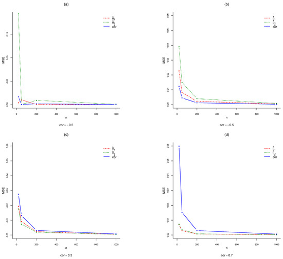
Figure 4. Summary of the results provided by lines of MSE of the estimates ${\widehat{\theta }}_1, {\widehat{\theta }}_2,$ and $\widehat{cor}$ for the different simulated data sizes n = 20, 50, 200, 1000 relating to the models (a) ZDBP ($0.30,1.57, 0.05),$ (b) ZDBP ($0.54,0.89, 0.07)$, (c) ZDBP ($0.44,0.37, 0.19),$ and (d) ZDBP ($0.17,0.19, 0.13)$.

2.2.4. Applications

Real data examples were studied to investigate the performance of the ZDBP model for fitting positively and negatively correlated bivariate data compared to other models.

Health and Retirement Study (HRS) Data

The first data set used to illustrate the application of the ZDBP model was drawn from the tenth wave of the Health and Retirement Study (HRS). A summary of the descriptive statistics of dependent variables for this data are provided by Islam and Chowdhury [26]. In the same study, bivariate Poisson-Poisson (BP-P) and bivariate right-truncated Poisson-Poisson (BRTP-P) models are fitted to the data from the Health and Retirement Study. The variables comprise the number of conditions a patient has ever had, as noted by doctors, X₁, and the utilization of healthcare services, where the services derive from hospitals, nursing homes, doctors, and home care assistants, X₂. The sample size is 5567 and the correlation between X₁ and X₂ is 0.06.

For the current study, the proposed ZDBP model was fitted to the same data and compared with the models in [26]. Table 5 summarises results for the fittings for the ZDBP model, the bivariate Poisson model with independent marginals (BP), and the BP-PR and the BRTP-P models. These results are shown in terms of the number of parameters used, and according to the Akaike Information Criteria (AIC), Bayesian Information Criteria (BIC), and loglikelihood estimate ($\ell )$. The results show the superiority of the ZDBP model for fitting the Health and Retirement Study (HRS) data in comparison with the other models, based on AIC and BIC, show the ability of the ZDBP model to fit positively correlated data. An analysis of the ML estimates derived for the ZDBP model is presented in Table 6.

Table 5. Comparison between models from the Health and Retirement Study data.

Model	AIC	BIC	$\mathit{\ell }$
ZDBP	31,727.26	31,747.14	−15,860.63
BP	32,707.61	32,720.86	−16,351.81
BP-P	33,419.33	33,432.58	−16,707.66
BRTP-P	33,196.42	33,209.67	−16,596.21

Table 6. Fitting Results for the ZDBP model from the Health and Retirement Study data.

Model	Parameter	Estimate	SE
Parameter	$p_{11}$	0.582	0.006
	${\theta }_1$	2.768	0.023
	${\theta }_2$	0.545	0.013
	cor	0.588

Australian Health Data (1977–1978)

The data discussed in this example comes from the Journal of Applied Econometrics 1997 Data Archive [27]. The data covers 5190 single-person households, and provides healthcare service utilization information from the 1977–1978 Australian Health Survey. A study by [28] uses this data in their analysis of various measures of health-care utilisation. A detailed summary of the statistics for the dependent and explanatory variables of this data is provided in [28]. We consider the number of consultations with doctors during the two-week period prior to the survey (Y₁) and the number of prescribed medicines used in the past 2 days (Y₂). The mean and the standard deviation of Y₁ are 0.302 and 0.798, respectively. The corresponding values for Y₂ are 0.863 and 1.415 and the correlation between Y₁ and Y₂ is 0.31.

The ZDBP model was fitted to the data and compared with the BP model. Table 7 presents a summary of results for the ZDBP and BP models, in terms of the number of parameters, AIC, BIC, and $\ell$. The results show the superiority of the ZDBP model compared with the BP model for fitting the Australian Health data, based on AIC and BIC. An analysis of the ML parameter estimates derived for the ZDBP model is shown in Table 8. In addition, we consider the dependent variables, Y₂, and the number of non-prescribed medications used in past two days, Y₃. The mean and the standard deviation of Y₂ are 0.863 and 1.42, the corresponding values for Y₃ are 0.356 and 0.71, and the correlation between Y₂ and Y₃ is −0.04. Table 9 presents a summary of the results for the ZDBP and BP models, in terms of the number of parameters, AIC, BIC, and $\ell$. The results show that the ZDBP model appears to be competitive with the BP model for fitting the Australian Health data in comparison with the other models, based on AIC and BIC. Therefore, this example emphasises the ability of the ZDBP model to fit positively and negatively correlated data. An analysis of the ML estimates derived for the ZDBP model is provided in Table 10.

Table 7. Comparison between the ZDBP and BP models from the Australian Health data.

Model	AIC	BIC	$\mathit{\ell }$
ZDBP	22,498.39	22,518.05	−11,246.19
BP	23,176.13	23,189.24	−11,586.07

Table 8. Fitting results for the ZDBP model from the Australian Health data.

Model	Parameter	Estimate	SE
Parameter	$p_{11}$	0.261	0.006
	${\theta }_1$	0.367	0.009
	${\theta }_2$	0.891	0.013
	cor	0.252

Table 9. Comparison between ZDBP and BP models from the Australian Health data.

Model	AIC	BIC	$\mathit{\ell }$
ZDBP	23,543.50	23,563.16	−11,768.75
BP	23,541.73	23,554.84	−11,768.86

Table 10. Fitting results for the ZDBP model from the Australian Health data.

Model	Parameter	Estimate	SE
Parameter	$p_{11}$	0.172	0.006
	${\theta }_1$	0.862	0.013
	${\theta }_2$	0.354	0.009
	cor	−0.01

3. Zero-Dependent Bivariate Poisson Regression Model (ZDBPR)

In this section, the Bivariate Bernoulli Poisson Regression Model will be considered. In this context, ${\alpha }_k=z_i^T{\beta }_{kl}$, $k=1,2,$ and 3 is where $z_i$ denotes a vector of explanatory variables of length l for the i-th observation related to the k-th parameter. This means that ${\beta }_{kl}$ is the corresponding vector of regression coefficients. In this respect, the ZDBPR model can take the following form:

$$\left.\begin{array}{c}\left(Y_{1i},Y_{2i}\right)~\mathrm{ZDBPR}\left({\theta }_{1i},{\theta }_{2i}, p_{11i}\right)\\ p_{11i}=\frac{e^{{\alpha }_{1i}}}{D}, p_{10i}=\frac{e^{{\alpha }_{2i}}}{D},p_{01i}=\frac{e^{{\alpha }_{3i}}}{D},p_{00i}=\frac{1}{D}\end{array}\right\}$$

(5)

where $D=1+e^{{\alpha }_{1i}}+e^{{\alpha }_{2i}}+e^{{\alpha }_{3i}}, P\left(B_j=0\right)=p_{01i}+p_{00i}=e^{-{\theta }_{ji}}, j=1,2$, and $i=1,2,\cdots ,n$ and $n$ denotes the observation number.

The ZDBPR model uses two response variables that are positively and negatively correlated. In addition, this model can be compared with other models to show that it has identical AIC, BIC, and parameter estimates.

3.1. Applications

3.1.1. Health and Retirement Study (HRS) Data

In this example, the same dependent variables used by [26] were considered, as outlined in “Health and Retirement Study (HRS) Data” Section. A study by [26] fit this data using bivariate right-truncated Poisson-Poisson regression (BRTP-PR), and bivariate Poisson-Poisson regression (BP-PR) models. They found that the BRTP-PR model appears to be significantly better than the BP-PR model for fitting the data.

For the purpose of this research, the ZDBPR model was used to fit the data, and was compared with the model used by [26]. Furthermore, the ZDBPR model was compared with the joint bivariate Poisson regression (JBPR) model used by [13], in which the covariates are gender (1 male, 0 female), age (in years), race (1 Hispanic, 0 others), and veteran status (1 yes, 0 no). Table 11 shows the results for the ZDBPR, JBPR, BPR, BP-PR, and BRTP-PR models in terms of the number of parameters, i.e., AIC, BIC, and $\ell$. The results show the superiority of the ZDBPR model for fitting the Health and Retirement Study data in comparison with the other models, based on AIC and BIC. This suggests that the ZDBPR model is able to fit positively correlated data. An analysis of the ML estimates derived for this model is provided in Table 12.

Table 11. Comparison between models for the Health and Retirement Study data.

	Number of Parameters	AIC	BIC	$\mathit{\ell }$
ZDBPR	15	31,982.88	32,082.25	−15,976.44
JBPR	15	32,524.53	32,623.90	−16,247.26
BPR	15	32,514.53	32,580.77	−16,247.26
BP-PR	15	33,192.13	33,258.38	−16,586.07
BRTP-PR	15	33,021.41	33,087.66	−16,500.71

Table 12. Fitting results for the ZDBPR model from the Health and Retirement Study data.

Parameter	Covariate	Coefficient	SE
${\alpha }_1$	constant	−0.471	0.591
	gender	0.014	0.063
	age	3.265	0.804
	Hispanic	−0.107	0.090
	Veteran	0.209	0.072
${\alpha }_2$	constant	−2.295	0.655
	gender	−0.528	0.072
	age	5.716	0.889
	Hispanic	0.201	0.093
	Veteran	−0.011	0.088
${\alpha }_3$	constant	−15.164	135.930
	gender	−2.239	706.157
	age	2.519	19.098
	Hispanic	−0.166	417.107
	Veteran	−1.296	1572.270

3.1.2. Australian Health Data (1977–1978)

In this example, the same dependent variables as used by [13] are used, namely Y₁ and Y₂. The covariates used are gender (1 female, 0 male), age in years divided by 100 (measured as midpoints of age groups), and the annual income in Australian dollars divided by 1000 (measured as midpoint of coded ranges). In the study by [13], model (A) was fitted as a JBPR model, where the covariates were gender, age, income, and age multiplied by gender, with gender as a covariate on the covariance scale. In addition, model (B) was fitted as a JBPR model, where the covariates were gender, age, and income, with a constant covariance term. A study by [13] concludes that the JBPR model performs better than the other models examined in their study. For the purposes of this current research, Model A and B have been fitted for the ZDBPR model. Table 13 shows the results for the ZDBPR and JBPR models, relating to the number of parameters, AIC, BIC, and $\ell$. These results show the superiority of the ZDBPR model for fitting the Health Care Australia data in comparison with the JBPR model, based on AIC and BIC. This suggests that the ZDBPR model can positively fit the correlated data. An analysis of the ML estimates derived for this model is provided in Table 14.

Table 13. Comparison between ZDBPR and JBPR models from the Health Care Australia data.

	Model	Number of Parameters	AIC	BIC	$\mathit{\ell }$
ZDBPR	A	15	19,856.41	19,954.73	−9913.21
JBPR		12	19,912.90	19,991.55	−9944.45
ZDBPR	B	12	19,910.80	19,989.45	−9943.40
JBPR		11	19,942.16	20,014.26	−9960.08

Table 14. Fitting results for the ZDBPR model from the Health Care Australia data using Model A.1 and B.1.

Model		A		B
Parameter	Covariate	Coefficient	SE	Coefficient	SE
	constant	−3.161	0.170	−2.670	0.127
	gender	5.980	0.298	4.780	0.177
	age	1.621	0.184	0.762	0.073
	income	−0.531	0.110	−0.509	0.106
	Age∗gender	−1.963	0.361
${\alpha }_2$	constant	−2.302	0.212	−2.202	0.188
	gender	0.894	0.491	0.430	0.324
	age	0.547	0.263	0.254	0.123
	income	−0.133	0.167	−0.105	0.167
	Age∗gender	−0.974	0.657
${\alpha }_3$	constant	−3.371	0.158	−2.798	0.116
	gender	6.031	0.286	4.589	0.162
	age	2.065	0.167	1.139	0.069
	income	−0.101	0.089	−0.076	0.091
	Age∗gender	−2.196	0.341

This current study also considered the same dependent variables used by Zamani et.al. [29], which are Y₂ and Y₃. Furthermore, [29] fit their data using a bivariate Poisson regression model, whereby the j.p.d is proposed by [5]. The bivariate Poisson model developed by [5] is defined from the product of two Poisson marginals with a multiplicative factor parameter. For ease of notation, the current study will refer to the Zamani et al. model as BPR [29]. Table 15 shows that the ZDBPR model performs better than the BPR [29] model in terms of AIC and BIC. This suggests that the ZDBPR model can fit negatively correlated data. Table 16 provides an analysis of the ML estimates derived for this model.

Table 15. Comparison between ZDBPR and BPR [29] models from the Health Care Australia data.

	Number of Parameters	AIC	BIC	$\mathit{\ell }$
ZDBPR	39	19,025.4	19,281.03	−9473.70
BPR [29]	26	19,097.2	19,267.60	−9522.59

Table 16. Results from fitting the ZDBPR model to the Health Care Australia data.

Parameter	Covariate	Coefficient	SE
${\alpha }_1$	constant	−5.791	0.349
	gender	1.383	0.110
	age	6.083	1.785
	agesq	−4.448	1.970
	income	0.323	0.152
	levyplus	0.442	0.126
	freepoor	−0.036	0.293
	freerepa	0.243	0.173
	illness	0.695	0.032
	actdays	0.097	0.014
	hscore	0.080	0.020
	chcond1	1.217	0.118
	chcond2	1.569	0.155
${\alpha }_2$	constant	−3.278	0.251
	gender	0.949	0.071
	age	1.737	1.343
	agesq	1.674	1.481
	income	0.052	0.110
	levyplus	0.225	0.089
	freepoor	−0.165	0.205
	freerepa	0.277	0.122
	illness	0.463	0.032
	actdays	0.077	0.014
	hscore	0.056	0.017
	chcond1	1.098	0.077
	chcond2	1.541	0.114
${\alpha }_3$	constant	−2.422	0.283
	gender	0.348	0.084
	age	5.403	1.671
	agesq	−6.079	1.946
	income	0.083	0.122
	levyplus	−0.145	0.089
	freepoor	−0.083	0.179
	freerepa	−0.449	0.167
	illness	0.344	0.032
	actdays	−0.010	0.020
	hscore	0.054	0.020
	chcond1	0.312	0.089
	chcond2	0.067	0.164

4. Conclusions

This paper has presented new bivariate Poisson models that can be fitted to bivariate and correlated count data with and without covariates. The main advantage of the ZDBP model and the ZDBPR model is their ability to fit positively and negatively correlated count data. This advantage is valuable for fitting different kinds of data in the healthcare field, as in the case of healthcare data, dependence between the two variables may be positive or negative. The statistical properties of the ZDBP model were discussed, and some properties of this model were proven, which shows that the pair of ZDBP variables can be positively or negatively correlated. Estimation for the ZDBP model was achieved using the ML and the MM methods, with different parameters, and with positive and negative correlations. In the simulation, the ML method showed good performance for estimation in comparison with the MM. Real data were used to examine the performance of the ZDBP model and the ZDBPR model for fitting positive and negative correlated count data, in comparison with other models. The applications for both models show the superiorities of these models in comparison with other models. This suggests that the ZDBP model and the ZDBPR model can allow the correlation structure to be positive or negative. Finally, although the proposed model was applied in two healthcare data sets, the model can be generalized and utilized in the other areas of research as well.

References

- Islam, M.A.; Chowdhury, R.I. Models for bivariate count data: Bivariate poisson distribution. In Analysis of Repeated Measures Data; Springer: Berlin/Heidelberg, Germany, 2017; pp. 97–124. [Google Scholar]
- Ghosh, I.; Marques, F.; Chakraborty, S. A new bivariate poisson distribution via conditional specification: Properties and applications. J. Appl. Stat. 2021, 48, 3025–3047. [Google Scholar] [CrossRef] [PubMed]
- Jung, R.C.; Winkelmann, R. Two aspects of labor mobility: A bivariate poisson regression approach. Empir. Econ. 1993, 18, 543–556. [Google Scholar] [CrossRef]
- Kocherlakota, S.; Kocherlakota, K. Bivariate Discrete Distributions; CRC Press: Boca Raton, FL, USA, 2017. [Google Scholar]
- Lakshminarayana, J.; Pandit, S.N.; Srinivasa Rao, K. On a bivariate poisson distribution. Commun. Stat.-Theory Methods 1999, 28, 267–276. [Google Scholar] [CrossRef]
- Marshall, A.W.; Olkin, I. A family of bivariate distributions generated by the bivariate bernoulli distribution. J. Am. Stat. Assoc. 1985, 80, 332–338. [Google Scholar] [CrossRef]
- Ma, Z.; Hanson, T.E.; Ho, Y.Y. Flexible bivariate correlated count data regression. Stat. Med. 2020, 39, 3476–3490. [Google Scholar] [CrossRef]
- Lee, H.; Cha, J.H.; Pulcini, G. Modeling discrete bivariate data with applications to failure and count data. Qual. Reliab. Eng. Int. 2017, 33, 1455–1473. [Google Scholar] [CrossRef]
- Campbell, J. The poisson correlation function. Proc. Edinb. Math. Soc. 1934, 4, 18–26. [Google Scholar] [CrossRef]
- Benz, L.S.; Lopez, M.J. Estimating the change in soccer’s home advantage during the COVID-19 pandemic using bivariate poisson regression. Adv. Stat. Anal. 2021, 1–28. [Google Scholar] [CrossRef]
- Koopman, S.J.; Lit, R. A dynamic bivariate poisson model for analysing and forecasting match results in the english premier league. J. R. Stat. Soc. Ser. A 2015, 178, 167–186. [Google Scholar] [CrossRef]
- Chou, N.-T.; Steenhard, D. Bivariate count data regression models—A sas® macro program. Stat. Data Anal. Pap. 2011, 355, 1–10. [Google Scholar]
- AlMuhayfith, F.E.; Alzaid, A.A.; Omair, M.A. On bivariate poisson regression models. J. King Saud Univ.-Sci. 2016, 28, 178–189. [Google Scholar] [CrossRef]
- Su, P.-F.; Mau, Y.-L.; Guo, Y.; Li, C.-I.; Liu, Q.; Boice, J.D.; Shyr, Y. Bivariate poisson models with varying offsets: An application to the paired mitochondrial DNA dataset. Stat. Appl. Genet. Mol. Biol. 2017, 16, 47–58. [Google Scholar] [CrossRef]
- Bermúdez, L.; Karlis, D. A posteriori ratemaking using bivariate poisson models. Scand. Actuar. J. 2015, 2017, 148–158. [Google Scholar] [CrossRef]
- I Morata, L.B. A priori ratemaking using bivariate poisson regression models. Insur. Math. Econ. 2009, 44, 135–141. [Google Scholar] [CrossRef]
- Holgate, P. Estimation for the bivariate poisson distribution. Biometrika 1964, 51, 241–287. [Google Scholar] [CrossRef]
- Mardia, K.V. Families of Bivariate Distributions; Lubrecht & Cramer Limited: Port Jervis, NY, USA, 1970. [Google Scholar]
- Johnson, N.L.; Kotz, S.; Balakrishnan, N. Discrete Multivariate Distributions; Wiley: New York, NY, USA, 1997. [Google Scholar]
- Inouye, D.I.; Yang, E.; Allen, G.I.; Ravikumar, P. A review of multivariate distributions for count data derived from the poisson distribution. Wiley Interdiscip. Rev. Comput. Stat. 2017, 9, e1398. [Google Scholar] [CrossRef]
- Weems, K.S.; Sellers, K.F.; Li, T. A flexible bivariate distribution for count data expressing data dispersion. Commun. Stat.-Theory Methods 2021, 1–27. [Google Scholar] [CrossRef]
- Cameron, A.C.; Trivedi, P.K. Regression Analysis of Count Data; Cambridge University Press: Cambridge, UK, 2013. [Google Scholar]
- Hofer, V.; Leitner, J. A bivariate sarmanov regression model for count data with generalised poisson marginals. J. Appl. Stat. 2012, 39, 2599–2617. [Google Scholar] [CrossRef]
- Famoye, F.; Consul, P. Bivariate generalized poisson distribution with some applications. Metrika 1995, 42, 127–138. [Google Scholar] [CrossRef]
- Berkhout, P.; Plug, E. A bivariate poisson count data model using conditional probabilities. Stat. Neerl. 2004, 58, 349–364. [Google Scholar] [CrossRef]
- Islam, M.A.; Chowdhury, R.I. A generalized right truncated bivariate poisson regression model with applications to health data. PLoS ONE 2017, 12, e0178153. [Google Scholar] [CrossRef] [PubMed]
- Australian Bureau of Statistics. Australian Health Survey 1977–78: Outline of Concepta; Methodology and Procedures Used (Cat. No. 4323.0); Australian Bureau of Statistics: Sydney, Australia, 1982. [Google Scholar]
- Cameron, A.C.; Trivedi, P.K.; Milne, F.; Piggott, J. A microeconometric model of the demand for health care and health insurance in Australia. Rev. Econ. Stud. 1988, 55, 85–106. [Google Scholar] [CrossRef]
- Zamani, H.; Faroughi, P.; Ismail, N. Bivariate generalized poisson regression model: Applications on health care data. Empir. Econ. 2016, 51, 1607–1621. [Google Scholar] [CrossRef]
Disclaimer/Publisher’s Note: The statements, opinions and data contained in all publications are solely those of the individual author(s) and contributor(s) and not of MDPI and/or the editor(s). MDPI and/or the editor(s) disclaim responsibility for any injury to people or property resulting from any ideas, methods, instructions or products referred to in the content. |
© 2023 by the authors. Licensee MDPI, Basel, Switzerland. This article is an open access article distributed under the terms and conditions of the Creative Commons Attribution (CC BY) license (https://creativecommons.org/licenses/by/4.0/).