Abstract
Low-temperature plasma is a new agricultural green technology, which can improve the yield and quality of rice. How to identify the harvest rice grown by plasma seed treatment plays an important role in the popularization and application of low-temperature plasma in agriculture. This study collected hyperspectral data of harvest rice, including plasma seed treated rice, and constructed a recognition model based on the hyperspectral image (HSI) by 3D ResNet (HSI-3DResNet), which extracts spatial spectral features of HSI data cubes through 3D convolution. In addition, a spectral channels 3D attention module (C3DAM) is proposed, which can extract key features of spectra. Experiments showed that the proposed C3DAM can improve the recognition accuracy of the model to 4.2%, while the size and parameters of the model only increase by 4.1% and 3.8%, respectively. The HSI-3DResNet proposed in this study is superior to other methods with the overall accuracy of 97.47%. At the same time, the algorithm proposed in this paper was also verified on a public dataset.
MSC:
68T07
1. Introduction
With the continuous increase of population, the contradiction between population and food production is increasingly prominent, especially in developing countries. Although global food security has been improved in recent years, many countries still suffer from serious food security problems [1]. Especially since the outbreak of COVID-19, food production has been greatly impacted, causing humanity to realize the importance of ensuring food security once again [2]. So far, pesticides and fertilizers have become important means to increase agricultural output. However, they also have harmful impacts on ecosystems, food safety and human health. As one of the world’s three major food crops, rice can provide complex carbohydrates, fiber, minerals, and vitamins. At present, most rice was planted through the use of pesticides and fertilizers to ensure the yield, which leads to the decline of rice quality. Therefore, a novel approach is needed to increase the productivity and quality of rice.
Plasma is the fourth state of matter [3], consisting of electrons, ions, radicals, ground state and excited atoms and molecules [4,5]. Low-temperature plasma (LTP), which can be obtained at room temperature and atmospheric pressure, has been widely used in agricultural application researches including treating seeds to promote germination and plant growth. For plasma seed treatment [6,7,8], the atmospheric pressure plasma, which contains large amounts of active components such as ozone, hydroxyl radical, nitric oxide, nitrogen dioxide, nitrous acid and so on, can positively affect the surface properties of seeds in a short treatment time, including etching the seed coat, and improving seed surface wettability and the entry of water and oxygen, which are essential factors for seed germination. In addition, in the process of plasma generation, the activity of some enzymes in seeds can be enhanced. Thus, seed germination, plant growth and nutrients can be accordingly improved [9]. For rice planting, the use of LTP technology can produce higher-quality rice. However, there is great lack of a relevant model for the effective identification of plasma-treated rice. The combination of computer vision and spectroscopy can be used in rice identification. Hyperspectral imaging (HSI) shows the spectral and spatial image information at the same time, which is a fast, efficient, accurate and nondestructive detection method. In this paper, the model based on HSI and 3D deep residual network was developed for the effective identification of rice grown by plasma seed treatment.
Although HSI was originally developed for remote sensing, with the development of technology, it has been applied to the detection of food including wheat grain hardness [10], water content [11] and protein content [12], as well as other quality traits. In addition, HSI has also been used for germination detection [13], and the prediction of alpha amylase activity [14] and parasitic contamination [15]. Gao Z. et al. [16] used HSI to detect grape leaf roll disease and showed that HSI technology has great potential in the non-destructive detection of virus infection in grape plants during the asymptomatic period. In the study of Wang H. et al. [17], HSI was used to detect tomatoes with early decay, showing that 100% of rotten tomatoes and 97.5% of healthy tomatoes could be identified by HSI. The study of Hu N. et al. [18] showed that HSI could well predict the trace element content of wheat including Ca, Mg, Mo and Zn. Khamsopha D. et al. [19] determined the content and adulteration of cassava starch by HSI.
In recent years, the use of hyperspectral detection in rice classification has also been studied. Combining the spectral and image spatial features, the seed data of six types of rice are classified and the classification accuracy can reach up to 84% [20]. Kong et al. [21] classified the HSI of four types of rice with the accuracy 90.67% using 12 selected characteristic wavelengths by the K-nearest neighbor (KNN) method. Wang et al. [22] used HSI to identify three types of rice seeds. The chalkiness, shape and spectral characteristics of rice were considered, and the classification accuracy reached 94.45%. Liu et al. [23] classified the HSI of three types of rice from the spectral information of a single seed using a support vector machine model, and the classification accuracy of the model reached 95.78%. In the study [24], a method of combining an artificial fish swarm algorithm and feature fusion was proposed, and then support vector machine was used to classify five kinds of rice seeds with the fused features. The classification accuracy of this method was as high as 99.44%. In the study [21], the author used HSI and random forest classifier to classify four kinds of rice seeds, and the classification accuracy could reach 100%. Recently, researchers have studied the classification of rice by different combinations of spectrum, texture, and morphological features [20,25].
Due to the complex data structure of hyperspectral images, the traditional feature extraction method (for example, [20,21,22,23,24,25]) requires high professional knowledge or experience and the high cost of feature extraction. Deep learning provides a good solution for the feature extraction of hyperspectral images. In 2012, Krizhevsky et al. [26] used GPU to train a CNN model for the classification task of the ImageNet dataset, and the model achieved the classification accuracy of 62.5%, which was higher than other methods at that time. This research had a huge impact in the field of image classification and target detection. With the development of deep learning, CNN [26], deep belief network (DFN) [27], stacked auto encoder (SAE) [28,29], deep residual network (ResNet) [30] and other deep learning network models are constantly being proposed. The deep learning methods have been gradually introduced into the field of hyperspectral image classification and achieved breakthrough progress. Ghamisi et al. [31] and Chen et al. [32] proposed a model for processing spectral data based on standard 1D CNN. Zhao and Du [33] used 2D CNN to extract spatially related features and proposed a classification method based on HSI spectral–spatial features. Zhang et al. [34] and Yang et al. [35] combined the spectral features extracted by 1D CNN and the spatial correlation features extracted by 2D CNN, and then used the softmax classifier for the final classification. In some studies, the DensNet model has been used to handle some HSI-related tasks. For example, Paoletti et al. [36] implemented a deep dense CNN model, which can be used to classify the spectral–spatial features of HSI data. Wang et al. [37] used DensNet to analyze the spectral, spatial, and spectral–spatial features of HSI data to achieve the classification. Fang et al. [38] proposed an end-to-end 3D DenseNet to extract the spectral–spatial features of HSI to enhance the classification effect.
The growth and quality of plasma-treated rice are different from that of ordinary rice, and there is a lack of dataset and classification model for plasma-treated rice. Therefore, this article is dedicated to solving these problems. The main novelties and contributions of this paper are as follows.
- (1)
- A hyperspectral image dataset of three kinds of rice was constructed. The dataset contains a total of 21,708 samples of three groups.
- (2)
- A spectral channels 3D attention module (C3DAM) is proposed, which can extract key features more effectively and improve the recognition accuracy.
- (3)
- The proposed model (HSI-3DResNet) can effectively identify the three groups of rice with the average accuracy of 97.46%.
2. Dataset Description
The construction of a plasma rice dataset met the following challenges. First, we conducted the treatment experiment of plasma on rice seeds and completed the field planting of the entire growth cycle of rice. Second, after harvesting, the original hyperspectral images of the threshed rice were obtained. Third, HSI images had to be preprocessed, including deleting useless background information and data correction.
2.1. Data Collection
The rice variety used for data collection was Nanjing 9108 (japonica), which was planted in Taizhou City, Jiangsu Province, China with the longitude and latitude of E119.97 and N32.64. The planting period of this kind of rice is from May to November. The experimental data were divided into three groups, namely group CK for local farms with traditional planting methods (using pesticides and chemical fertilizers), group C with only organic carbon fertilizer during planting, and group P (or plasma group) only with plasma treatment. In the rice planting experiment, rice seeds were treated by arc discharge with 455 W and using air as the reaction gas with the gas flow rate of 1.5 L/min and the treatment time of 1.2 s. All the rice groups grew to natural maturity for harvest. The seed treatment and rice planting process are shown in Figure 1. First, LTP technology was used to treat rice seeds, and the growth process included several stages of seedling breeding, transplanting, field management and rice harvest.
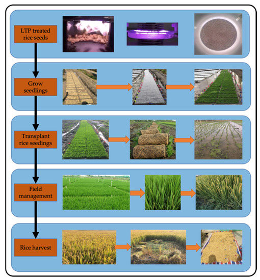
Figure 1.
Flow chart of rice treatment and planting.
A total of 1 kg harvested rice samples were randomly selected in each group for hyperspectral detections. HSIs of rice samples were collected using a visible-near-infrared reflectance hyperspectral imaging system, as shown in Figure 2. The GaiaSorter HSI system used in this study includes a uniform light source, spectral camera, electronically controlled mobile platform, computer and control software, etc. The system is available in three standard spectral bands, 400–1000, 900–1700 and 1000–2500 nm, and is equipped with small conveyor belts for continuous small-batch measurements. The system uses a bromine tungsten lamp as its light source, which emits uniform light through thermal radiation. The light source adopts the trapezoidal structure design of four bulbs, and the light intensity of the upper and lower bulbs is controlled and adjusted the with knobs, so that the light uniformity is higher than 90% in the volume of 300 × 20 × 100 mm3. Figure 2a shows the physical diagram of the GaiaSorter system. Figure 2b shows the structure diagram including (1) the hyperspectral imager, (2) diffuse light source, (3) working distance regulator, (4) electric mobile platform, (5) electric lifting platform and (6) computer position.
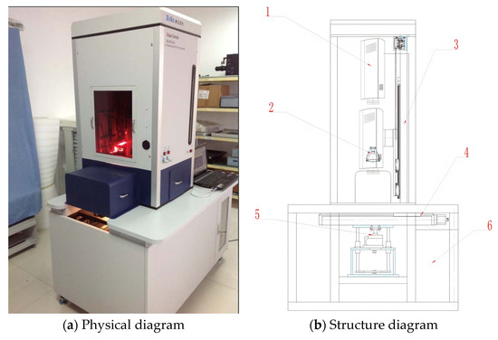
Figure 2.
Near infrared hyperspectral imaging data collection system: (a) the physical diagram of the GaiaSorter system; (b) the structure diagram, including 1—hyperspectral imager; 2—diffuse light source; 3—working distance regulator; 4—electric mobile platform; 5—electric lifting platform; and 6—computer position.
In this study, we selected the standard spectral band of 400–1000 nm, with a total of 176 wavelength data. During the collection of rice hyperspectral image data, every 250 g of rice was evenly placed on the blackboard, which was put into the HSI system for data collection. The resolution of the HSI data collected in the experiment was 960 × 1440 × 176. In the experiment, 15 pieces of original rice HSI data were collected, including 5 pieces of CK, C and P data each. Figure 3(a1–c1) show the HIS data for group CK (a1), group C (b1) and group P (c1). Here, the 1024 curves with different colors in each of Figure 3(a3–c3) show the spectral curves in a area (i.e., each pixel has its individual spectral curve marked by one color).
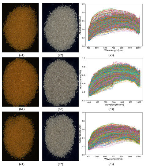
Figure 3.
Data of rice: the original calibrated image data and rice spectra of group CK (a1–a3), group C (b1–b3) and group P (c1–c3). The original image data collection was illuminated with halogen lamps.
Three-dimensional hyperspectral images of rice were obtained by linear scanning. It can be represented by , where and represent space dimensions and spectral dimensions. Five HSI images were collected for each type of rice. In order to reduce the influence of noise and illumination instability, it is necessary to correct the black and white plates of hyperspectral images. The correction method is shown in Equation (1).
where and are the spectral strength of images before and after correction, respectively, and and are the spectral strength of the black and white board images, respectively. Figure 3(a2–c2) show the calibrated HSI images of groups CK(a2), C(b2) and P(c2). In this paper, we used the calibrated data as experimental data. Figure 3(a3–c3) show the spectra of the three types of rice with 1024 spectral curves in each group. From Figure 3(a3–c3), it can be seen that the spectral curve of the plasma group is obviously more compact than groups CK and C. In group CK, more spectral curves distribute in the region of less than 700 nm, while those of group C mainly distribute in the region of larger than 700 nm. The differences between these spectra indicates that the identification and classification of different groups of rice can be achieved by the different features of hyperspectral data.
2.2. Data Preprocessing
Figure 4 shows the three main steps of dataset construction in this study, which are data collection, data selection and data augmentation. Step 1 is data collection, including sample selection and hyperspectral image data collection, as described in Section 2.1. Step 2 is data selection. The rice image are concentrated in the range of 896 × 1280 pixels in the middle of the HSI. The effective HSI data are selected for clipping and then divided into segments with the size of 128 × 128 pixels. Therefore, each original hyperspectral image of rice can be divided into 70 segments with 128 × 128 pixels. Step 3 is data augmentation. Since the neural network model is prone to overfitting, it is necessary to perform some data augmentation operations in the training phase in order to obtain a high-precision CNN-based model [39]. Due to the high dimension of HSI data, it has high requirements for computer equipment. Meanwhile, in order to increase the number of data samples, the data cube needs to be cropped. Random cropping is one of the most effective data augmentation methods. A slice randomly cut from the original training image was input to the model during training, which enriched the diversity of the model’s training data. Together with random flipping, random cropping and its variants were intensively applied to the current research on HSI classification and recognition algorithms [40]. Through data crop, the hyperspectral image data were randomly cropped into 25 hyperspectral images of 32 × 32 pixels and the unusable data (whose rice pixels do not account for more than a quarter of the data cube) were removed. Through the above three steps, a usable rice HSI dataset with 21,708 data samples was constructed, including 7540 pieces of group CK, 7216 pieces of group C and 6952 pieces of group P, as shown in Table 1. The data is stored in mat format with the shape of 32 × 32 × 176.
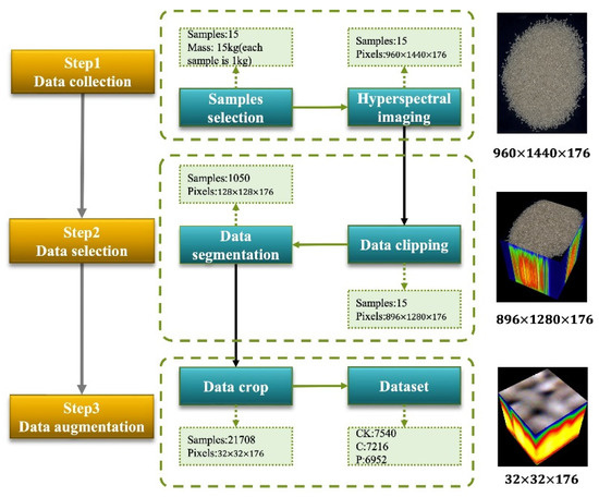
Figure 4.
Data processing flow chart.

Table 1.
The number and proportion of each rice class in the dataset.
3. HSI Recognition Model Based on 3DResNet (HSI-3DResNet)
3.1. Spectral Channels 3D Attention Module (C3DAM)
Since the attention model was proposed, it has been widely used in deep learning. The structure of the spectral channels 3D attention module (C3DAM) proposed in this paper is shown in Figure 5, and it can be embedded into other backbone networks such as ResNet, DenseNet, and the latest ConvNext to enhance the ability of extracting key features and accordingly enhance the classification accuracy of the models. C3DAM is a computational unit that can be built upon a transformation mapping an input to feature maps , as shown in Equation (2). In the map, there are convolution, batch normalization (BN), sigmoid and max pool operations.
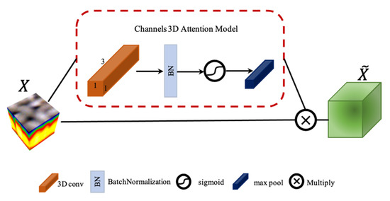
Figure 5.
C3DAM structure. The red dotted box is the attention mechanism model proposed in this paper.
In the study of this paper, rice image features (color, contour, shape, background and so on) can be well extracted by 3D convolution. Due to different substances exhibiting different spectra, the spectral characteristics of HSI data of rice are complex due to the different groups of rice and the diversity of rice components. It is necessary to improve the spectral feature extraction ability. In this study, a 3D convolution kernel was used to extract spatial features of HSI. denotes the output of the convolution operation and denotes the learning set of the filter kernel. Then, can be expressed as Equation (3), where represents the convolution calculation.
Through the convolution calculation, the data features on the channel are extracted so as to enhance the sensitivity of features in the subsequent process. In this study, the convolution kernel was used. Through the batch normalization, sigmoid and max pool operations, the normalized features were enhanced to obtain the weights maps, as shown in Equation (4), where is the weights maps, σ is the sigmoid function and δ is the BN function.
After the weights maps were used to redistribute the weights of input, the feature maps with sensitive information enhancement were obtained, as shown in Equation (5), where is the multiplication.
3.2. Structure of HSI-3DResNet
The hyperspectral image includes two-dimensional spatial information and one-dimensional spectral information, which form a 3D data cube. In order to better obtain the spatial features and spectral features from HSI, 3D convolution, 3D batch normalization, 3D pooling operation and the Relu function are used in the proposed HSI-3DResNet.
The use of 3D convolution in the hyperspectral image data cube can perform 3D convolution calculations in the spatial domain and the spectral domain at the same time, so as to extract the spatial–spectral features of the data cube. The output of the convolution calculation for the input and the 3D convolution kernel () is defined as:
where represents the value of the element of output , the position of is , corresponds to the of HSI data in this paper, represents the bias, and () represents the size of stride in the 3D convolution. denotes the size of output , which is defined as:
where denotes the round-to-zero process. In general, stack multiple (maybe dozens or hundreds) of 3D convolution kernels on the same layer to discover various types of spectral–spatial features, and at the same time generate the same number of feature matrices.
In order to reduce the number of parameters of the neural network in the training process and improve the generalization ability of the model, a pooling layer is usually added to the network model. The 3D max pooling layer can be used for feature learning in tasks such as action recognition and target detection in video, and it can also be used for data feature learning in HSIs. The batch normalization is used after the convolution layer, where it adjusts the distribution of data and normalizes the output of each layer to a distribution with the mean of 0 and the variance of 1. This ensures the effectiveness of the gradient. Suppose is an input of a mini batch, where represents a piece of sample data, is the batch size, and is the output of 3D batch normalization; then, is defined as:
where and are learning ability parameters, ε is set to 1 × 10⁻⁵, is the mean value of the mini batch and is the variance of the mini batch, with the calculation formula shown in Equations (9) and (10).
In the convolutional neural network, as the number of layers of the network keeps increasing, the problem of network degradation will occur in the process of training. In order to solve this problem, He K. et al. proposed the ResNet network in 2015 [36]. ResNet introduced the residual learning framework into the network to establish the shortcut connections between layers so as to improve the backpropagation ability of the gradient during training, solve the problem of gradient disappearance, and thus improve the performance of the model. The formulation F(X) = F(X) + X is the mapping relationship of residual learning, as shown in Figure 6.
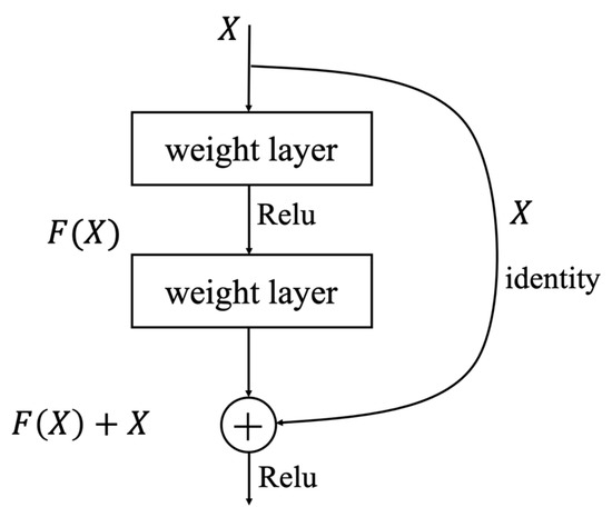
Figure 6.
Residual learning: a building block [30].
The basic block structure of HSI-3DResNet is shown in Figure 7. It includes two 3 × 3 × 3 convolutional layers and a C3DAM layer as well as two BNs and Relu operations. In this study, the 3D convolution kernel, 3D pooling and 3D BN were used to replace the original 2D parts, which enables the model to learn the spatial features and spectral features at the same time and is more suitable for the 3D data cubes of HSIs. In addition, the proposed C3DAM module based on an attention mechanism was added into the model, allowing key features to be learned by the model to obtain a higher accuracy.
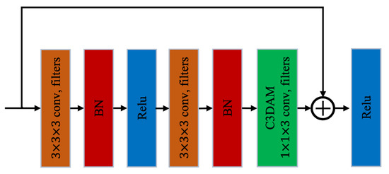
Figure 7.
A basic block of HSI-3DResNet.
The structure of HSI-3DResNet and ResNet is similar. Figure 8 shows the structure of HSI-3DResNet with different layers, where (a) shows HSI-3DResNet-18 and (b) shows HSI-3DResNet-34. The input of HSI-3DResNet is a 32 × 32 × 176 HSI data cube. Different from ResNet, the input data of HSI-3DResNet first undergoes C3DAM to redistribute the weights, and is then input into a convolution kernel size 5 × 5 × 5, filter 64, and stride 2 convolution layer. After that, the structure of HSI-3DResNet is similar to that of ResNet. In HSI-3DResNet, we used 3D max pooling and 3D average pooling to replace the 2D max pooling and 2D average pooling in ResNet, and replaced the ResNet Basic block structure with the HIS-3DResNet Basic block structure (shown in Figure 7).
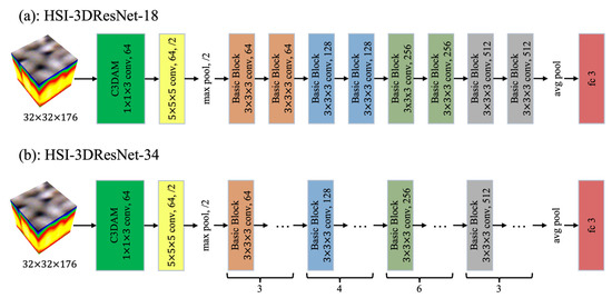
Figure 8.
HSI-3DResNet structure: (a) HSI-3DResNet-18 and (b) HSI-3DResNet-34.
4. Results and Discussion
4.1. Run Environment
Because the deep neural network training process has many iterations and a large number of matrix operations, which requires a large amount of computing resources, a high-performance graphics processing unit (GPU) is indispensable. In this experiment, NVIDIA GeForce RTX 3090 is used for model training, and its graphics memory is 24 GB. The CPU model is an Intel(R) Core (TM) i9-10900K (3.70 GHz) and the memory size is 128 GB. The operating system was Ubuntu18.04 and the model was implemented using Tensorflow2.4. The CUDA Toolkit 11.1 and CUDNN V8.0.4 were used for computation acceleration. Anaconda3.6 and Python3.8 are respectively the development environment and programming language for the model.
4.2. Evaluation Indicators
In this study, the following indicators were considered to evaluate the model. First of all, overall accuracy (OA) and average accuracy (AA) are widely used in the classification and identification tasks of HSI data [36]. However, they do not fully explain the performance of the model. Ka is a common index used for consistency checking (i.e., the prediction results of all classes are better) for HIS data and can be used for evaluating the classification effects of HSI data. The closer Ka is to 1, the better the consistency of classification. A confusion matrix, also known as an error matrix, is widely used in classification. It can clearly describe the actual category and predict the categories of each row and column. OA, AA and Ka are all calculated based on the confusion matrix.
where represents the classification quantity of the test sample, and , , and represent the true positive (TP), false positive (FP), false negative (FN) and true negative (TN) sample of the th class, respectively. The calculation formula of is shown in Equation (14).
where represents the number of samples in the test sample, represents the actual number of samples of the th class in the test sample, and denotes the number of prediction samples of the th class in the test sample.
4.3. Public Datasets
To verify the validity of the model, not only the constructed rice dataset was used, but also the public HSI dataset named Indian Pines (IP) was used. The IP images were captured by the AVIRIS sensor at the IP agricultural test site in northwest Indiana. The spatial resolution of the spectral image is 145 × 145. The available ground truths are divided into 16 categories. Table 2 shows the number of available samples for the IP HSI dataset.
Table 2.
Number of available samples in the Indian Pines (IP) dataset.
4.4. Experiments’ Results
Before the model training started, 80% of the data in the dataset were randomly selected as the training set and the remaining 20% of the data were used as the validation set. The hyperparameter settings in the training process are shown in Table 3. Due to the Adam optimizer having a strong optimization ability with adaptive moment estimation, it allows a small learning rate. In addition, the proposed attention module C3DAM can enhance the extraction ability of key features and find the gradient direction more accurately during training, which also allows a small learning rate. Thus, the learning rate was set as the fixed low value of 1 × 10⁻⁴.
Table 3.
Hyperparameter table.
In the model training process, standard cross-entropy [41] is used as the loss function and it is defined as in Equation (15).
where y and denote the expected and actual outputs, respectively.
The difference between HSI-3DResNet and 3DResNet is that C3DAM is added to HSI-3DResNet to better learn the important features in the HSI data cube. The experiment compared the recognition result of the four models of 3DResNet-18, HSI-3DResNet-18, 3DResNet-34 and HSI-3DResNet-34 on different datasets.
Table 4 shows the recognition results of the four models on the rice dataset and IP dataset. By comparing OA, AA and Ka of different models, we found that HSI-3DResNet-34 obtained the best recognition effect for the two datasets. The OA of HSI-3DResNet-34 on the rice dataset and IP dataset was the highest, reaching 97.46% and 99.95%, respectively. At the same time, by comparing the recognition results of the models between HSI-3DResNet-34 and 3DResNet-34 (or the models between HSI-3DResNet-18 and 3DResNet-18) on different datasets, we found that adding the C3DAM module to the model can improve the recognition performance of the model. The improvement was more prominent on the rice dataset constructed in this paper. For example, after adding the C3DAM module, the overall accuracy of HSI-3DResNet-34 on the rice dataset was 4.24% higher than that of the model 3DResNet-34, and the overall accuracy of HSI-3DResNet-18 was 2.33% higher than that of the model 3DResNet-18.
Table 4.
The recognition results of 3DResNet-18, HSI-3DResNet-18, 3DResNet-34 and HSI-3DResNet-34 on the rice dataset and IP dataset.
In the model training, the model size and parameter quantities of the four models were also compared, as shown in Figure 9. For example, the impacts of adding and not adding the proposed C3DAM module on the model size and parameter quantities of 3DResNet with 34 and 18 layers was compared, which were 440.1, 422.8, 231.1 and 220.6, respectively. Their parameter quantities were 10.9, 10.5, 5.7 and 5.5 million in order. This shows that the adding of the C3DAM module to 3DResNet-34 and 3DResNet-18 causes an increase of model size by 4.1% and 4.8%, respectively, and an increase of parameter quantities by 3.8% and 3.6%, respectively, and accordingly the accuracy improved by 4.24% and 2.33%, respectively. Without considering the C3DAM module, the model size and parameter quantities of 3DResNet-34 were 2.0 and 1.9 times those of 3DResNet-18, respectively, while when adding the C3DAM module, the model size and parameter quantities of 3DResNet-18 were only about half of 3DResNet-34 (without adding C3DAM module), but the accuracy was 1.007 times that of 3DResNet-34, which shows the significant role of the proposed C3DAM module.
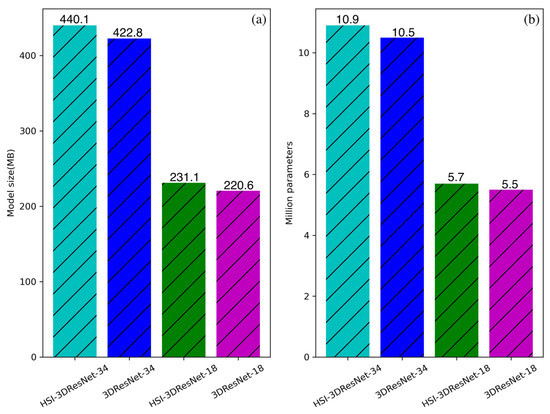
Figure 9.
Comparison of model size (a) and parameters amount (b).
In the model testing, we randomly selected 4342 samples (80%) from the original dataset as the test set including 1508 for group CK, 1443 for group C and 1391 for group P. In Figure 10, the confusion matrix of the four models is calculated. The real category (ordinate) is compared with the predicted category (abscissa) to describe the recognition accuracy of the models. From Figure 10a, it can be seen that HSI-3DResNet-34 had the highest individual recognition accuracy, with the accuracy of 96.883% for CK, 98.406% for C and 97.124% for P. The individual accuracy of three groups of rice by HSI-3DResNet-34 was higher than that by 3DResNet-34. For plasma rice recognition, the accuracy of HSI-3DResNet-18 was higher than 3DResNet-34, showing the accuracy improvement of the C3DAM module.
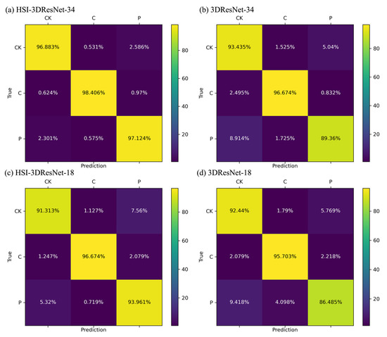
Figure 10.
Confusion matrix of the testing results. (a) HSI-3DResNet-34; (b) 3DResNet-34; (c) HSI-3DResNet-18; (d) 3DResNet-18.
In the experiment, in addition to the above four models, the recognition results by the 11 models were also compared, including the original ResNet-34, ResNet-18 and 1D CNN, and some traditional machine learning methods such as XGBoost, support vector machine (SVM), multiple linear regression (MLR) and random forest (RF). Table 5 shows the recognition results of the 11 models on the public IP dataset and the rice dataset. It can be seen that the proposed model had the best recognition effects (marked in bold) on both the IP and the rice datasets, showing that our model has the highest OA, AA and Ka. At the same time, it can also be found that compared with traditional machine learning, deep learning has obvious advantages in the recognition task of HSI data.
Table 5.
Classification results of different models in the IP dataset and the rice dataset.
Figure 11 shows the recognition results of the IP dataset by different methods, where (a) is the ground reference map and (b)–(l) are the recognition results of the 11 methods. It is seen that the proposed method has the best recognition image, which is the closest to the original ground reference map with the accuracy of 99.95%.
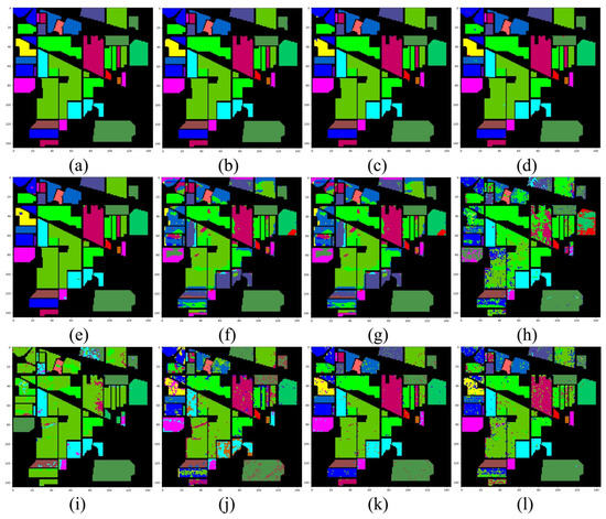
Figure 11.
Comparison of classification results on the Indian Pines (IP) dataset. (a) Ground-truth map; (b) HSI-3DResNet-34 (99.95%); (c) HSI-3DResNet-18 (99.85%); (d) 3DResNet-34 (99.71%); (e) 3DResNet-18 (99.61%); (f) ResNet-34 (70.39%); (g) ResNet-18 (56.41%); (h) CNN1D (73.36%); (i) SVM (99.71%); (j) RF (81.50%); (k) XGBoost (83.61%); (l) MLR (77.62%).
Figure 12 shows the classification results of the 11 models in the rice dataset. From Figure 12 and Table 5, it can be seen that the OA, AA and Ka of HSI-3DResNet-34 were the highest among all these models, with the OA of 97.46%, AA of 97.47% and Ka of 94.19%. MLR had the worst classification effect, less than 50%, indicating that MLR could not learn many useful features in the dataset. Due to the 3D convolution kernel’s ability to extract spatial and spectral features, it has a better learning ability for HSI data cubes. In addition, by comparing HSI-3DResNet and 3DResNet, it can be seen that adding the proposed C3DAM module can make the model learn more key features, so as to improve the accuracy of the model but not cause the obvious increase in the model size and parameters, which has been shown in Figure 9.
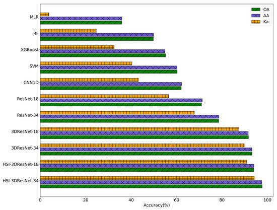
Figure 12.
Recognition results of different models in the rice dataset.
5. Conclusions
In this paper, plasma technology was used to treat rice seeds and a field plant experiment on the treated rice seeds was conducted. Hyperspectral images of three kinds of rice after harvest including plasma rice were collected and a HSI dataset of rice was constructed. A ResNet-based HSI data classification model, HSI-3DResNet, was constructed, and 3D convolution was used to extract spatial–spectral features. At the same time, a C3DAM attention module suitable for HSI data cubes was proposed, so that the model can learn more key spectral features, but the size of the model and the parameters will not increase significantly. The model established in this paper has achieved a good classification effect with the average accuracies of 97.47% on the rice dataset and 99.97% on the public IP dataset. These results indicate that the identification and classification of plasma rice can be effectively solved by constructing the HSI-3DResNet model. The model was also effectively applied to a public HSI dataset. This study is of great significance to the identification of LTP technology in agriculture.
Author Contributions
Conceptualization, X.T. and F.H.; methodology, X.T.; software, X.T., W.Z. and B.L.; validation, X.T., J.G. and Y.W.; formal analysis, X.L.; investigation, X.L.; resources, F.H.; data curation, X.T. and X.L.; writing—original draft preparation, X.T., F.H.; writing—review and editing, F.H.; visualization, Y.W.; supervision, F.H.; project administration, F.H.; funding acquisition, F.H. All authors have read and agreed to the published version of the manuscript.
Funding
This research was funded by the National Natural Science Foundation of China (No. 11675261 and 12075315) and the horizontal projects of China Agricultural University (No. 202105511011054 and 202005511011203).
Data Availability Statement
This study used the public datasets from http://www.ehu.eus/ccwintco/index.php/Hyperspectral_Remote_Sensing_Scenes (accessed on 10 November 2022) and rice dataset from the corresponding author.
Conflicts of Interest
The authors declare no conflict of interest.
References
- Food Security Information Network (FSIN). Global Report on Food Crises 2018, Executive Summary; Food Security Information Network (FSIN): Rome, Italy, 2018; ISBN 9788578110796. [Google Scholar]
- Guoqiang, C.; Mande, Z. COVID-19 pandemic is affecting food security: Trends, impacts and recommendations. China’s Rural. Econ. 2020, 5, 13–20. [Google Scholar]
- Crookes, W. Experiments on the dark space in vacuum tubes. Proc. R. Soc. A Math. Phys. Eng. Sci. 1907, 79, 98–117. [Google Scholar] [CrossRef]
- Tendero, C.; Tixier, C.; Tristant, P.; Desmaison, J.; Leprince, P. Atmospheric pressure plasmas: A review. Spectrochim. Acta Part B. At. Spectrosc. 2006, 61, 2–30. [Google Scholar] [CrossRef]
- Randeniya, L.K.; De Groot, G.J.J.B. Non-Thermal plasma treatment of agricultural seeds for stimulation of germination, removal of surface contamination and other benefits. A Review. Plasma Process. Polym. 2015, 12, 608–623. [Google Scholar] [CrossRef]
- Šerá, B.; Šerý, M.; Zahoranová, A.; Tomeková, J. Germination improvement of three pine species (Pinus) after diffuse coplanar surface barrier discharge plasma treatment. Plasma Chem. Plasma Process. 2020, 41, 211–226. [Google Scholar] [CrossRef]
- Mazandarani, A.; Goudarzi, S.; Ghafoorifard, H.; Eskandari, A. Evaluation of DBD plasma effects on barley seed germination and seedling growth. IEEE Trans. Plasma Sci. 2020, 48, 3115–3121. [Google Scholar] [CrossRef]
- Bormashenko, E.; Grynyov, R.; Bormashenko, Y.; Drori, E. Cold radiofrequency plasma treatment modifies wettability and germination speed of plant seeds. Sci. Rep. 2012, 2, 741. [Google Scholar] [CrossRef]
- Starič, P.; Vogel-Mikuš, K.; Mozetič, M.; Junkar, I. Effects of nonthermal plasma on morphology, genetics and physiology of seeds. A Review. Plants 2020, 9, 1736. [Google Scholar] [CrossRef] [PubMed]
- Mahesh, S.; Jayas, D.S.; Paliwal, J.; White, N.D.G. Comparison of partial least squares regression (PLSR) and principal components regression (PCR) methods for protein and hardness predictions using the Near-Infrared (NIR) hyperspectral images of bulk samples of canadian wheat. Food Bioprocess Technol. 2014, 8, 31–40. [Google Scholar] [CrossRef]
- Non-Destructive Prediction of Moisture of Wheat Seed Kernel by Using VIS/NIR Hyperspectral Technology; American Society of Agricultural and Biological Engineers: St. Joseph, MI, USA, 2016. [CrossRef]
- Caporaso, N.; Whitworth, M.B.; Fisk, I.D. Protein content prediction in single wheat kernels using hyperspectral imaging. Food Chem. 2018, 240, 32–42. [Google Scholar] [CrossRef] [PubMed]
- Alisaac, E.; Behmann, J.; Rathgeb, A.; Karlovsky, P.; Dehne, H.W.; Mahlein, A.K. Assessment of fusarium infection and mycotoxin contamination of wheat kernels and flour using hyperspectral imaging. Toxins 2019, 11, 556. [Google Scholar] [CrossRef]
- Xing, J.; Van Hung, P.; Symons, S.; Shahin, M.; Hatcher, D. Using a short wavelength infrared (SWIR) hyperspectral imaging system to predict alpha amylase activity in individual Canadian western wheat kernels. Sens. Instrum. Food Qual. Saf. 2009, 3, 211–218. [Google Scholar] [CrossRef]
- Singh, C.; Jayas, D.; Paliwal, J.; White, N. Detection of insect-damaged wheat kernels using near-infrared hyperspectral imaging. J. Stored Prod. Res. 2009, 45, 151–158. [Google Scholar] [CrossRef]
- Gao, Z.; Khot, L.R.; Naidu, R.A.; Zhang, Q. Early detection of grapevine leafroll disease in a red-berried wine grape cultivar using hyperspectral imaging. Comput. Electron. Agric. 2020, 179, 105807. [Google Scholar] [CrossRef]
- Wang, H.; Hu, R.; Zhang, M.; Zhai, Z.; Zhang, R. Identification of tomatoes with early decay using visible and near infrared hyperspectral imaging and image-Spectrum merging technique. J. Food Process. Eng. 2021, 44, e13654. [Google Scholar] [CrossRef]
- Hu, N.; Li, W.; Du, C.; Zhang, Z.; Gao, Y.; Sun, Z.; Yang, L.; Yu, K.; Zhang, Y.; Wang, Z. Predicting micronutrients of wheat using hyperspectral imaging. Food Chem. 2020, 343, 128473. [Google Scholar] [CrossRef] [PubMed]
- Khamsopha, D.; Woranitta, S.; Teerachaichayut, S. Utilizing near infrared hyperspectral imaging for quantitatively predicting adulteration in tapioca starch. Food Control. 2020, 123, 107781. [Google Scholar] [CrossRef]
- Vu, H.; Tachtatzis, C.; Murray, P.; Harle, D.; Dao, T.K.; Le, T.L.; Andonovic, I.; Marshall, S. Spatial and spectral features utilization on a hyperspectral imaging system for rice seed varietal purity inspection. In Proceedings of the 2016 IEEE RIVF International Conference on Computing & Communication Technologies, Research, Innovation, and Vision for the Future (RIVF), Hanoi, Vietnam, 7–9 November 2016; pp. 169–174. [Google Scholar] [CrossRef]
- Kong, W.; Zhang, C.; Liu, F.; Nie, P.; He, Y. Rice seed cultivar identification using near-Infrared hyperspectral imaging and multivariate data analysis. Sensors 2013, 13, 8916–8927. [Google Scholar] [CrossRef] [PubMed]
- Wang, L.; Liu, D.; Pu, H.; Sun, D.-W.; Gao, W.; Xiong, Z. Use of hyperspectral imaging to discriminate the variety and quality of rice. Food Anal. Methods 2014, 8, 515–523. [Google Scholar] [CrossRef]
- Liu, X.; Feng, X.; Liu, F.; He, Y. Identification of hybrid rice strain based on near-infrared hyperspectral imaging technology. Trans. Chin. Soc. Agric. Eng. 2017, 33, 189–194. [Google Scholar] [CrossRef]
- Sun, J.; Zhang, L.; Zhou, X.; Yao, K.; Tian, Y.; Nirere, A. A method of information fusion for identification of rice seed varieties based on hyperspectral imaging technology. J. Food Process. Eng. 2021, 44, e13797. [Google Scholar] [CrossRef]
- Sun, J.; Lu, X.; Mao, H.; Jin, X.; Wu, X. A method for rapid identification of rice origin by hyperspectral imaging technology. J. Food Process. Eng. 2015, 40, e12297. [Google Scholar] [CrossRef]
- Krizhevsky, A.; Sutskever, I.; Hinton, G.E. Imagenet classification with deep convolutional neural networks. Adv. Neural Inf. Process. Syst. 2012, 25, 1097–1105. [Google Scholar] [CrossRef]
- Hinton, G.E.; Osindero, S.; Teh, Y.-W. A fast learning algorithm for deep belief nets. Neural Comput. 2006, 18, 1527–1554. [Google Scholar] [CrossRef]
- Zhou, P.; Han, J.; Cheng, G.; Zhang, B. Learning compact and discriminative stacked autoencoder for hyperspectral image classification. IEEE Trans. Geosci. Remote Sens. 2019, 57, 4823–4833. [Google Scholar] [CrossRef]
- Zhou, S.; Xue, Z.; Du, P. Semisupervised stacked autoencoder with cotraining for hyperspectral image classification. IEEE Trans. Geosci. Remote Sens. 2019, 57, 3813–3826. [Google Scholar] [CrossRef]
- He, K.; Zhang, X.; Ren, S.; Sun, J. Deep residual learning for image recognition. In Proceedings of the IEEE Computer Society Conference on Computer Vision and Pattern Recognition (CVPR), Las Vegas, NV, USA, 27–30 June 2016; pp. 770–778. [Google Scholar] [CrossRef]
- Ghamisi, P.; Plaza, J.; Chen, Y.; Li, J.; Plaza, A.J. Advanced spectral classifiers for hyperspectral images: A review. IEEE Geosci. Remote Sens. Mag. 2017, 5, 8–32. [Google Scholar] [CrossRef]
- Wang, L.; Peng, J.; Sun, W. Spatial–spectral squeeze-and-excitation residual network for hyperspectral image classification. Remote Sens. 2019, 11, 884. [Google Scholar] [CrossRef]
- Zhao, W.; Du, S. Spectral–spatial feature extraction for hyperspectral image classification: A dimension reduction and deep learning approach. IEEE Trans. Geosci. Remote Sens. 2016, 54, 4544–4554. [Google Scholar] [CrossRef]
- Zhang, H.; Li, Y.; Zhang, Y.; Shen, Q. Spectral-spatial classification of hyperspectral imagery using a dual-channel convolutional neural network. Remote. Sens. Lett. 2017, 8, 438–447. [Google Scholar] [CrossRef]
- Yang, J.; Zhao, Y.; Cheung, J.; Chan, W.; Yi, C.; Brussel, V.U. Hyperspectral image classification using two-channel deep convolutional neural network. In Proceedings of the IEEE International Geoscience and Remote Sensing Symposium (IGARSS), Beijing, China, 10-15 July 2016; pp. 5079–5082. [Google Scholar]
- Paoletti, M.E.; Haut, J.M.; Plaza, J.; Plaza, A. Deep & Dense convolutional neural network for hyperspectral image classification. Remote Sens. 2018, 10, 1454. [Google Scholar] [CrossRef]
- Wang, W.; Dou, S.; Jiang, Z.; Sun, L. A fast dense spectral–spatial convolution network framework for hyperspectral images classification. Remote Sens. 2018, 10, 1068. [Google Scholar] [CrossRef]
- Fang, B.; Li, Y.; Zhang, H.; Chan, J.C.W. Hyperspectral images classification based on dense convolutional networks with spectral-Wise attention mechanism. Remote Sens. 2019, 11, 159. [Google Scholar] [CrossRef]
- Wu, X.; Sahoo, D.; Hoi, S.C.H. Recent advances in deep learning for object detection. Neurocomputing 2020, 396, 39–64. [Google Scholar] [CrossRef]
- Li, W.; Chen, C.; Zhang, M.; Li, H.; Du, Q. Data augmentation for hyperspectral image classification with deep CNN. IEEE Geosci. Remote Sens. Lett. 2018, 16, 593–597. [Google Scholar] [CrossRef]
- De Boer, P.T.; Kroese, D.P.; Mannor, S.; Rubinstein, R.Y. A tutorial on the cross-entropy method. Ann. Oper. Res. 2005, 134, 19–67. [Google Scholar] [CrossRef]


Disclaimer/Publisher’s Note: The statements, opinions and data contained in all publications are solely those of the individual author(s) and contributor(s) and not of MDPI and/or the editor(s). MDPI and/or the editor(s) disclaim responsibility for any injury to people or property resulting from any ideas, methods, instructions or products referred to in the content. |
© 2023 by the authors. Licensee MDPI, Basel, Switzerland. This article is an open access article distributed under the terms and conditions of the Creative Commons Attribution (CC BY) license (https://creativecommons.org/licenses/by/4.0/).