Design and Comparison of Fractional-Order Controllers in Flotation Cell Banks and Flotation Columns Used in Copper Extraction Processes

Abstract

This work explores efficiency improvements in the copper flotation stage, a complex nonlinear, multivariable process subject to numerous perturbations. The primary objective is to design a fractional-order PID (FOPID) control strategy and a fractional-order model reference adaptive control (FOMRAC) system. The parameters for these controllers are optimized using the particle swarm optimization (PSO) algorithm with an objective function tailored to the control goals. This study employs models of both a bank series of five flotation cells and a flotation column. Their performance results are compared against traditional controllers, such as an integer-order PID and MRAC. The findings reveal that fractional-order controllers offer notable advantages over their integer-order counterparts, showing improved performance metrics with minimal changes to the existing control framework. This research highlights the effectiveness of fractional control in enhancing flotation processes and introduces a novel application of fractional control techniques in this area.

1. Introduction

The first mention of fractional calculus dates back to 1695, where, in a conversation between Leibniz and L’Hopital, who was looking for the meaning of Leibniz’s notation ${\displaystyle \frac{d^{n}y}{d{x}^n}}$ (quite popular at the time) for the derivative of order $n\in {\mathbf{N}}_0:=\{0,1,2,\dots \}$ when: $n=1/2$ (what if $n=1/2$?), Leibniz replied “This is an apparent paradox from which, one day, useful consequences will be drawn”. Later mentions of fractional derivatives were made by Euler in 1730, Lagrange in 1772, Laplace in 1812, Lacroix in 1819, Fourier in 1822, Liouville in 1868, Sonin in 1869, Laurent in 1884, Nekrassov in 1888, Krug in 1890 and Weyl in 1917. The first text devoted to fractional calculus was by Oldham and Spanier [1] in 1974. Fractional calculus is a prominent area of research, as demonstrated in [2], where a new fractional dimensional reproduction kernel space (RKS) based on Caputo’s fractional derivative is introduced. Fractional calculus extends traditional calculus to non-integer orders, providing a mathematical foundation for fractional controllers [3,4]. Due to their unique advantages in managing complex and dynamic systems, fractional controllers are particularly compelling for applications in industries with intricate processes, such as mining.

The main incomes of countries such as Australia, Bolivia, Chile and Peru come from the mining industry. A critical component of mineral processing within the mining industry is the flotation stage, which plays a pivotal role in separating valuable minerals from mine tailings [5]. This process is especially crucial in the extraction of copper, where flotation is used to concentrate the copper ore, allowing for the recovery of high-purity material.

Given the importance of this stage, improving the control of flotation, particularly the level control, is of great significance. Enhanced control over the flotation process directly contributes to the production of purer material, which not only boosts the quality of the extracted minerals but also leads to economic benefits for the industry. By optimizing flotation control, mining operations can achieve higher efficiency, reduce waste, and ultimately increase profitability, making this a key area for technological advancements and research in mineral processing. There are different ways flotation can be carried out, such as by using a flotation cell bank or flotation column; this process has variable and very dynamic behavior, as it depends on changes in the characteristics of the mineral or the natural variation of a liquid when subjected to flow changes. The topics of flotation control, modeling, and related issues have been the focus of active research in recent years [6,7,8,9,10,11,12,13,14,15,16,17,18,19,20,21,22,23].

Despite the application of advanced control techniques in many industries, PID controllers are not commonly used in the mineral processing industry due to the difficulty in their implementation and the lack of a comprehensive performance comparison between different control strategies, leading to low motivation for their use in industry [24]. In the academic literature, there are many works that have applied model predictive control (MPC) and its variants, with promising results [7,11,16,17,22,25,26,27,28,29,30,31,32,33,34].

In the study presented in [25], an MPC problem was formulated to minimize the tracking error of the gas holdup and bias rate while ensuring that the gas flow rate, wash-water flow rate and bias rate remained within their operational limits. This work specifically focuses on the error in the tracking of the gas holdup. The work in [26] explores the design of an MPC system for a mineral column flotation process, which is modeled by a set of nonlinear coupled heterodirectional hyperbolic partial differential equations and ordinary differential equations. The results are demonstrated through simulations, with a complex mathematical model utilized to capture the dynamics of the process. The research in [27] presents a flotation column control system using an MPC applied to a three-phase system (air–water–ore) with data sourced from an industrial environment. The validation results showed a maximum accuracy of 75%, but the study did not include real-time optimization. The investigation in [28] developed a model based on an Artificial Neural Network (ANN) that uses two past values and one present value of the tailing valve opening, along with the interface level, as inputs to predict the future interface level. This model was utilized to design an MPC for controlling the interface level. The controller was tested on both liquid–gas and liquid–gas–solid systems. However, this work does not address a MIMO system, and the ANN requires a substantial amount of training data. The study in [35] aims to regulate the bubble size distribution (BSD) to a desired set point. The BSD was measured in real time using an image analysis method, and a dynamic nonlinear model (Wiener) based on a log-normal distribution was built for estimating the BSD. A constrained model predictive controller was then designed to control the BSD. This work was developed in an experimental laboratory setting, and further implementation is needed in terms of its image analysis component. The works in [30,34] design an MPC system using data extracted from real industries in Peru and Chile. These studies developed models that achieved a minimum accuracy of 70% for a cell bank flotation process and 83% for a flotation column process. The results demonstrated that the MPC models outperformed those obtained using PI controllers. The work in [16] is Part I and presents an exhaustive study on modeling a flotation cell, while Part II in [17] proposes an MPC strategy based on the previously developed model. The study in [22] conducted experimental laboratory tests to validate the findings of the previous simulated studies presented in [11,36]. This experimental approach provided a crucial step in the verification of the theoretical models and simulation results, offering practical insights and confirming the applicability of the proposed methods under controlled conditions.

On the other hand, MPC strategies (and different variants of these) for flotation cell banks were applied in [7,31,32,33,34]. Their simulation results were presented in [7,31,32,34] and they were then applied to a real industry. MPC controllers have a high cost and complexity to their implementation. Finally, in [37,38,39,40], other controllers (PI, steady-state control) were applied to simulation cases.

However, controllers such as PI, output regulation and Adaptive Decoupling (among others), have shown interesting results in [14,24,37,38,39,40]. Previous works have also dealt with flotation columns [14,19,24,25,26,27,28,29,30,37] and flotation cell banks [7,16,17,18,22,31,32,34,38,39,40].

Since an MPC relies heavily on the accuracy of a mathematical model for effective performance, even slight changes in the model, such as those with an ANN model, can lead to suboptimal results. An alternative, and more robust, approach to handling model variations is an adaptive control, such as an MRAC. This control has been used to control a flotation column [24] and compared with MPC and PI controllers; this study involves the design of an Adaptive Decoupling Controller (ADC) and compares its control performance with that of MPC and SISO PID controllers. The results indicated that, due to the weak coupling of variables in the studied case (as also reported by other researchers), the ADC achieved satisfactory control of the column, even outperforming the MPC in terms of various indices. This work was conducted on a pilot flotation column. In [24,25,26] an MPC (and different variants) was used to control the gas holdup, bias rate and concentration in a simulated flotation column. The development, implementation and evaluation of an MPC for the control applied to a flotation column was presented in [24,27,28,29,30], while a pilot flotation column was used in [24,27,28,29,30] before these were applied to a real industry.

All the mentioned works utilize mathematical models, except for [27,30,34], and present results from simulations or laboratory experiments. However, they fall short in bridging the gap to their real-world implementation. Furthermore, none of these studies specifically focus on fractional controllers for this particular process.

Finally, this paper has the following novelties:

• To optimize the process for both a series-connected flotation cell bank and a flotation column, mathematical models have been derived from real operating plants [30,34]. The primary approach of this work is to utilize this relevant information to design fractional controllers based on data from actual industrial processes.
• The design of FOPID and FOMRAC controllers is proposed for both a flotation cell bank and a flotation column. Unlike previous research, which has primarily focused on traditional or model-based controllers, this work explores the application of fractional controllers to these processes. The novelty of this approach lies in its application of fractional-order control techniques to flotation systems, a domain where such methods have not been previously implemented. By leveraging fractional calculus, this research aims to enhance the control performance and robustness of flotation processes, providing a new perspective on optimizing these complex systems.
• A comparison of our fractional controllers, a FOPID controller and a FOMRAC, was carried out, determining the gains of both controllers via particle swarm optimization (PSO) and comparing these with that of their integer counterparts.

Therefore, after analyzing the results of comparisons based on the performance indexes of two plants, it can be concluded that the fractional controllers generally offer significant advantages over integer controllers. Notably, the fractional reference model controller demonstrates exceptional performance in the flotation cell bank, showcasing a substantial improvement over the other controllers. This advantage is reflected in various performance metrics, highlighting the efficacy of fractional controllers in achieving better control and stability in these processes.

We recommend several avenues for future research, including the real-world implementation or laboratory testing of fractional calculus and controllers. Additionally, exploring the discretization of fractional calculus and controllers will be essential for their practical application. Furthermore, we suggest investigating alternative optimization techniques beyond PSO to enhance the design and performance of fractional controllers.

This paper begins with Section 2, which introduces the fundamental concepts of fractional control, including fractional-order PID control and fractional-order model reference adaptive control, and provides an overview of the flotation process. Section 3 details the modeling of both the flotation cell bank and flotation column, outlining the methodologies and parameters used. Section 4 presents a comparative analysis of different controllers, including their tuning with PSO and the results from simulations using cell bank flotation and column flotation. Finally, Section 5 summarizes the conclusions drawn from the study, reflecting on the performance of fractional controllers and suggesting directions for future research.

2. Preliminaries

This section presents the basic concepts of the fractional-order calculus which will be used in this study. Following the main basic definitions of FO operators (FOOs), the fractional-order PID (FOPID) and the fractional-order MRAC (FOMRAC) control strategies are described.

2.1. Fractional Control Concepts

We will first review the basic definitions associated with fractional calculus. An extensive review of the basic theoretical concepts of fractional calculus can be found in [41,42,43,44]. Fractional calculus is a generalization of classical calculus that extends the concept of derivatives and integrals to non-integer (fractional) orders. It provides tools for describing and analyzing processes that exhibit memory and hereditary properties which are not adequately captured by traditional integer-order models [41].

The fundamental operators representing fractional-order differentiation (FOD) and fractional-order integration (FOI) are denoted by $D^{\alpha }$, where $\alpha \in \mathrm{R}$ is the order of differentiation or integration. Thus, the FO derivative and integral operators are denoted as

$$D^{\alpha }=\left\{\begin{array}{cc}{\displaystyle \frac{d^{\alpha }}{d{t}^{\alpha }}},\hfill & \alpha >0,\hfill \\ 1,\hfill & \alpha =1,\hfill \\ \int {\left(d\tau \right)}^{\alpha },\hfill & \alpha <0.\hfill \end{array}\right.$$

(1)

There exist several alternative definitions of FOD, such as those given by Weyl, Fourier, Cauchy, Abel, and Nishimoto, among others. However, the three most used definitions of FOD are the Grunwald–Letnikov (GL), the Riemann–Liouville (RL), and the Caputo (C) FO derivatives [44]. These last three definitions are equivalents under some conditions for a large class of functions [41]. In this study we will make use the FO derivative according to Caputo, since it is the most used in engineering applications.

A Caputo derivative of order $\alpha$ of a function $f\left(t\right)$ with respect to time is defined by

$${\hspace{0.17em}}_a{D}_t^{\alpha }f\left(t\right)={\displaystyle \frac{1}{\Gamma (n-\alpha )}}{\int }_{\alpha }^t{\displaystyle \frac{f^{\left(n\right)}\left(\tau \right)}{{(t-\tau )}^{\alpha -n+1}}}d\tau ,$$

(2)

with $n-1\le \alpha <n$.

Caputo’s definition has the advantage of adequately dealing with the initial conditions (ICs), since they are given in terms of IO derivatives of the function. This is one of the reasons to use Caputo’s derivative in this study. In the following sections, we present the main properties of the fractional-order PID (FOPID) control and its fractional order.

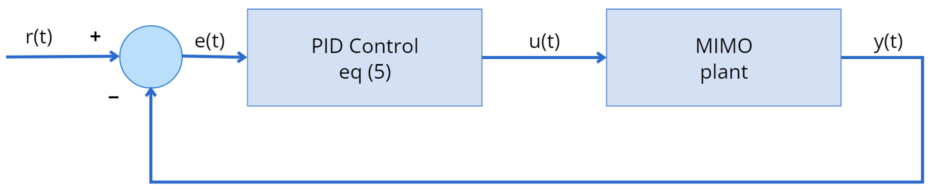
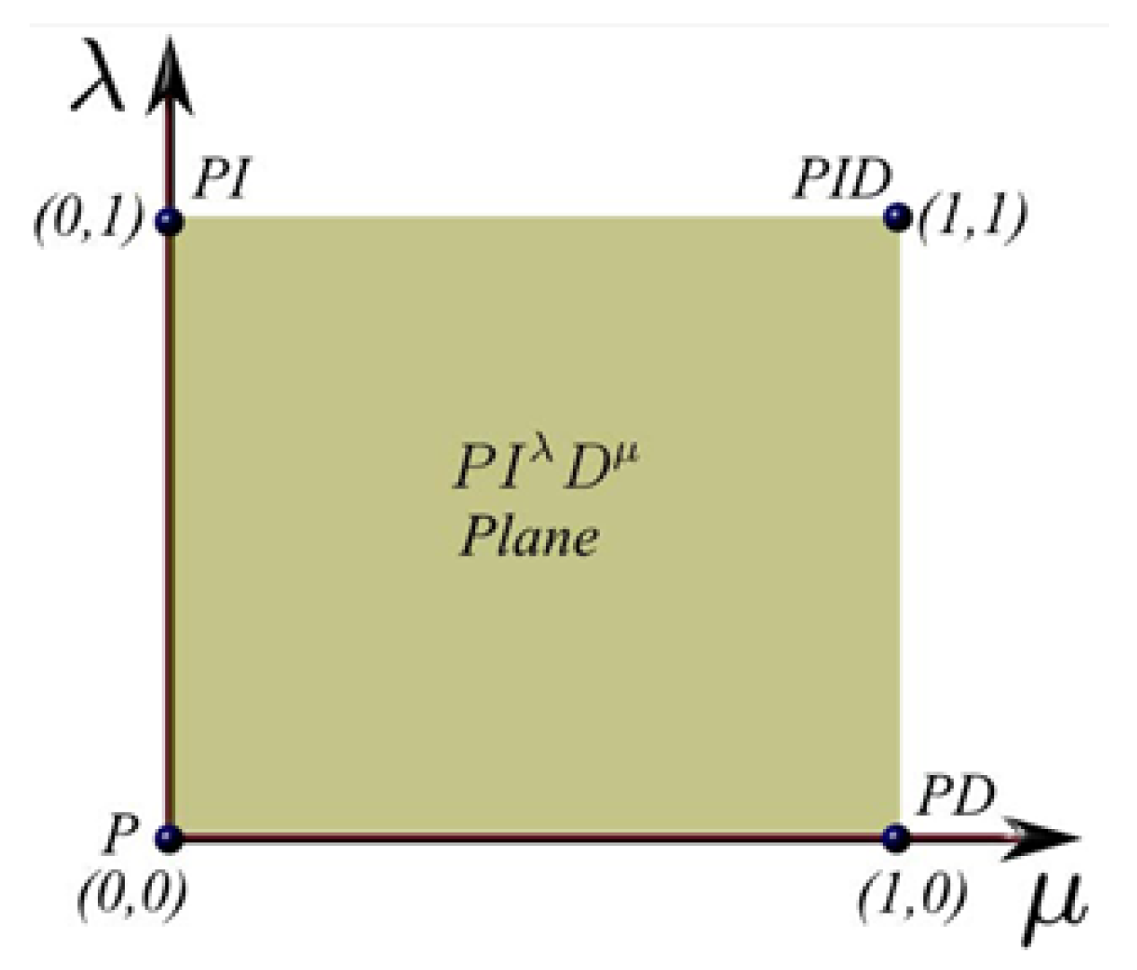
2.2. Fractional-Order PID Control

This section first describes the basis of the classical IOPID [44,45] and then states the theory of FOPID controllers, the foundation of which was developed in [6,44]. Next, we present a controller design based on [46] and its corresponding stability analysis [47,48]. Discrete FOPID controllers [49] and the latest advances in FO control [35] are then presented. Figure 1 presents a block diagram of the PID controller used in the system.

The transfer function of the IOPID controller is given by

$$C_1\left(s\right)=K_p+{\displaystyle \frac{K_i}{s}}+K_{d}s,$$

(3)

where $\{K_p,K_i,K_d\}$ are the controller’s gains.

The generalization that corresponds to the FOPID associated with the FO derivative of order $\mu$ and the FO integral of order $\lambda$ is given by

$$C_2\left(s\right)=K_p+{\displaystyle \frac{K_i}{s^{\lambda }}}+K_d{s}^{\mu },$$

(4)

where $\{\lambda ,\mu \}$ are positive real numbers, typically in the interval (0,2). For $\lambda =1$ and $\mu =1$, the FOPID controller’s structure reduces to that of the classic IOPID controller. Other controller variants like FOPI or FOPD can also be obtained by making $\lambda =0$ or $\mu =0$.

Thus, the control action in the time domain would be [41,44]

$$u\left(t\right)=K_{p}e\left(t\right)+K_i{D}^{-\lambda }e\left(t\right)+K_d{D}^{\mu }e\left(t\right).$$

(5)

Figure 2 ([44], pag. 50) shows the regions in the $\{\lambda ,\mu \}$ plane associated with all possible combinations of $\lambda \in [0,1]$ and $\mu \in [0,1]$ for the IOPID and FOPID controllers. It is evident that the IOP, IOPI, IOPD and IOPID controllers are only four points in the $\{\lambda ,\mu \}$ plane and that FOPID controllers can use any values inside the plane, offering more alternatives for them to control the system than the standard IOPID controllers, i.e., the FOPID controller can be seen as a generalization of the classic IOPID controller. Therefore, with this approach the designer has infinite degrees of freedom to choose the parameters of the controller. Note that classical IOPID controllers can only reach the four corners of the square in Figure 1. This FO approach has been applied to model ultracapacitors in the frequency domain [50], in the level control of conical tank [36] and in the control of a position servo with a time delay [8], among other applications.

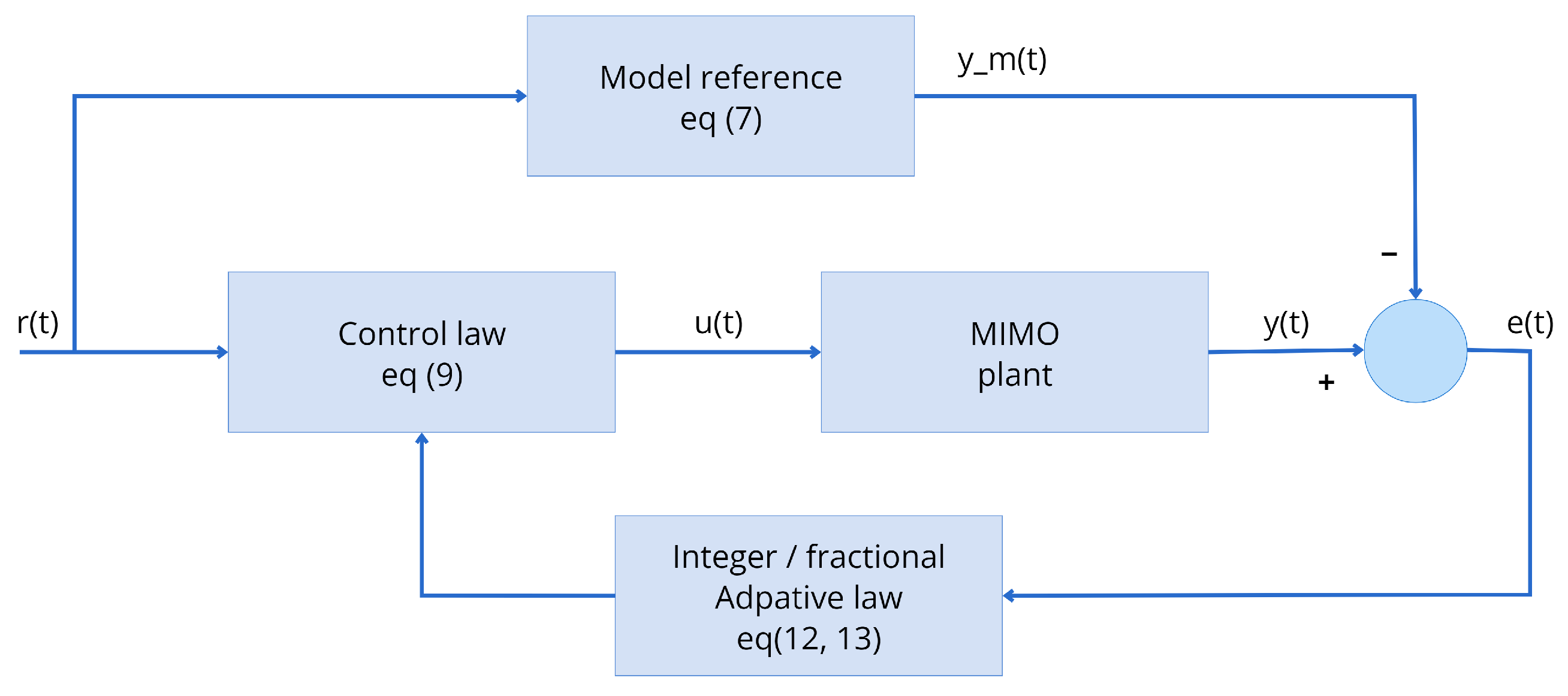
2.3. Fractional-Order Model Reference Adaptive Control

This section briefly describes the FOMRAC technique that will be used to control a copper flotation cell bank and a copper column flotation, due to the characteristics and importance of these mining processes. The MRAC technique has been widely developed and applied in MIMO systems [10,45,51], multivariable plants with delays [52], plants with the partial feedback of their states or little information given [52,53], autoregressive models [9], nonlinear systems [54], discrete multivariables [55], a multivariate MRAC designed using generalized passivation [56], and second-order systems [57].

Let us consider a linear MIMO time-invariant plant (TI) with m inputs and m outputs, defined as

$$y\left(t\right)=G_0\left(s\right)u\left(t\right),$$

(6)

where $G_0\left(s\right)$ is an unknown rational transfer matrix and $y\left(t\right)\in R^m$ and $u\left(t\right)\in R^m$ are the vectors of the outputs and inputs of the plant, respectively.

The objective of the MRAC is to find a feedback control vector $u\left(t\right)$ for a continuous-time plant (6) with unknown plant parameters such that $y\left(t\right)$ tracks a given reference signal $y_m\left(t\right)$ as closely as possible and the resulting closed-loop system is globally stable in the sense that all signals in the system are uniformly bounded for any bounded initial conditions. The reference model is given by

$$y_m\left(t\right)=W_m\left(s\right)r\left(t\right),$$

(7)

where $W_m\left(s\right)$ is a known given mxm strictly proper and stable transfer matrix and $r\left(t\right)\in R^m$ is any piecewise, continuous uniformly bounded known signal.

To achieve such an objective, the following standard assumptions are made about the plant transfer function $G_0\left(s\right)$:

• $G_0\left(s\right)$ is any transfer function of a full-rank, stable and minimum phase (i.e., all zeros of $G_0\left(s\right)$ are in the left half of the complex plane).
• The upper bound $\overline{v}$ on the observability index v of $G_0\left(s\right)$ is known.
• The high-frequency gain matrix $K_p$ of $G_0\left(s\right)$ is such that $S{K}_p$ is a symmetric and positive definite matrix for some known matrix S.
• The modified left interactor matrix of $G_0\left(s\right)$ is a lower triangle polynomial matrix denoted as $\xi \left(s\right)$.

Figure 3 presents a block diagram of the MRAC controller.

The MRAC controller depicted in Figure 2 utilizes a reference model matrix, which is selected as follows:

$$W_m\left(s\right)={\xi }_m^{-1}\left(s\right)$$

(8)

Considering that $\xi \left(s\right)$ is not unique and $r\left(t\right)$ can be realized through input dynamics, there is a lot of flexibility in choosing the model’s dynamics.

The controller structure is chosen to be

$$u\left(t\right)={\theta }_1^T{\omega }_1\left(t\right)+{\theta }_2^T{\omega }_2\left(t\right)+{\theta }_{20}^{T}y\left(t\right)+{\theta }_3^{T}r\left(t\right)$$

(9)

where ${\omega }_1\left(t\right)={\displaystyle \frac{A\left(s\right)}{n\left(s\right)}}\left[u\right]\left(t\right)$ and ${\omega }_2\left(t\right)={\displaystyle \frac{A\left(s\right)}{n\left(s\right)}}\left[y\right]\left(t\right)$.

Some auxiliary equations are given by

$$\zeta \left(t\right)=h\left(s\right)I\left[\omega \right]\left(t\right)$$

(10)

$$\epsilon \left(t\right)=\tilde{K}\left(t\right)\xi \left(t\right)+K^{*}{\tilde{\theta }}^T\left(t\right)\zeta \left(t\right)$$

(11)

such that the fractional-order adjustment laws are given by

$${\dot{\Theta }}^{\alpha }\left(t\right)={\displaystyle \frac{-S^T\epsilon \left(t\right){\zeta }^T\left(t\right)}{1+{\zeta }^T\left(t\right)\zeta \left(t\right)+{\xi }^T\left(t\right)\xi \left(t\right)}}$$

(12)

$${\dot{K}}^{\alpha }\left(t\right)={\displaystyle \frac{-\Gamma \epsilon \left(t\right){\xi }^T\left(t\right)}{1+{\zeta }^T\left(t\right)\zeta \left(t\right)+{\xi }^T\left(t\right)\xi \left(t\right)}}$$

(13)

In a fractional MRAC system in a plant (6) subject to the previously described assumptions, the model (7), the controller (9) with the fractional adaptive laws (12) and (13), all uniformly bounded signals and the tracking error $e\left(t\right)=y\left(t\right)-y_m\left(t\right)$ go to zero asymptotically with time.

The stability of the FOMRAC system, specifically in relation to the Caputo derivative, has been rigorously demonstrated and proven in prior works [3,4,58]. These studies present comprehensive theorems that establish the uniform stability of fractional-order systems within the Lyapunov framework. The proofs provided in these references reinforce the robustness of the FOMRAC, ensuring that the system maintains stability under the influence of fractional dynamics, which is critical for the effective control of such systems during their practical application.

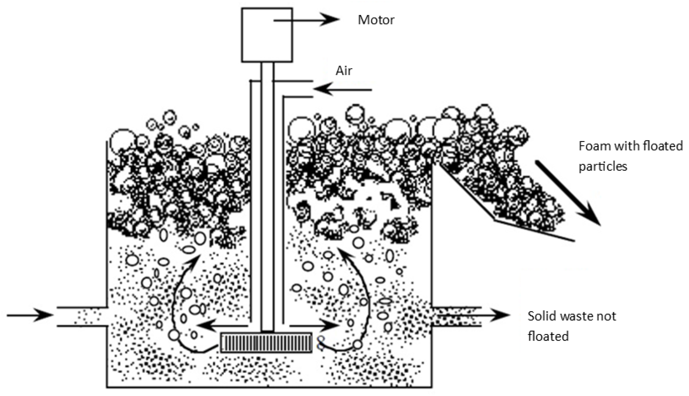
2.4. Flotation Process

Copper mineral processing can be divided in two sectors; the mine and the concentrator plant. Inside the concentrator plant, the processes can vary, but they can be summarized into the following steps [34]: primary crushing, grinding, flotation, thickness filters and concentration.

The flotation stage is quite important since allows us to separate the copper from the rock using its so-called aerophilic property [59]. This property allows some materials to adhere more easily to air bubbles than others, so that the valuable material floats and unusable materials remain at the bottom of the cell [60].

The basic unit used for this process is called a flotation cell or flotation column. This is a tank or vessel of different dimensions depending on the amount of material that needs to be processed. The so-called “pulp material”, which comes from the previous stage of the process where the rock is ground and mixed with water, enters into this tank, cell or column, which has two outputs; the first one is where the concentrate of the valuable material (in this case, copper) comes out and the other one is where the remaining material (poor-in-value material) is extracted.

To carry out this process, some chemicals (foaming agents and collectors) are added. These greatly facilitate this process. In the units (tank or column), there is a scraper connected to a motor that drives air and generates movement to generate bubbles. Thus, the valuable material can rise and be removed due to overflow.

The objective is to control the pulp level so that the froth overflows the cell border in a controlled way. This material moves to the next stage and the remaining material can be passed to another cell or tank. Figure 4 presents the cell flotation process.

3. Model Description

The methodology employed in this study utilizes data from a real process referenced in previous research to design fractional-order controllers specifically tailored to operating around the process’s operational point. The key advantage of this approach is that it enables the development of controllers that are directly applicable to real-world scenarios, enhancing their practical relevance. However, one of the main challenges of this method is the difficulty in experimentally validating the proposed controllers.

The two controllers described in Section 2.2 and Section 2.3 will be developed to carry out this process in both a flotation cell bank and flotation column. Notably, the information used for modeling was sourced from prior studies. The model of the flotation cells, based on data from a real industrial process in Chile, was obtained from [34], while the model of an industrial process in Peru was derived from [30].

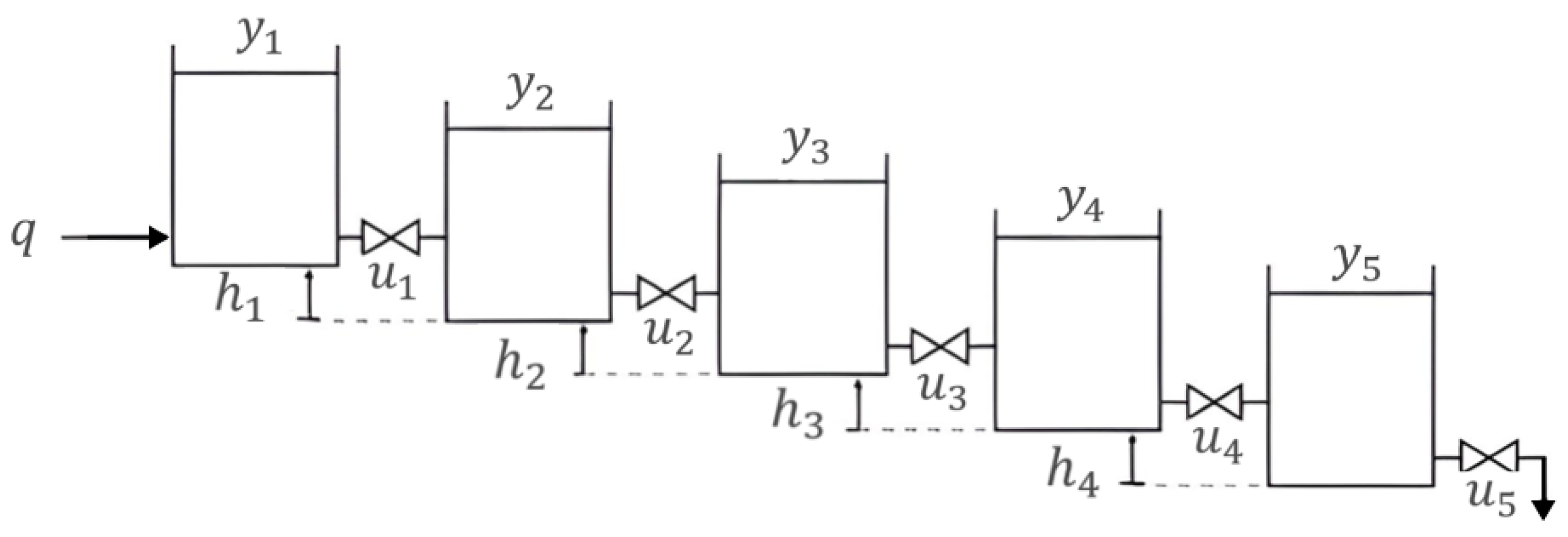
3.1. Flotation Cell Bank Modeling

In this section, a linear mathematical model obtained from the identification system in [34] is employed. The data were extracted from an operational mine, so this mathematical model is a very useful approximation of real behavior. Although the mentioned project works with two lines in parallel, in this work only line 1 will be considered. The simulated plant has five flotation cells in series, each one of 3000 [ft3] capacity, as shown in Figure 5.

For each cell, we determined the transfer functions and ended up with five linearized SISO systems in series, which were expressed in the state space, forming a MIMO system.

The representation of the five cells using state variables is given below:

$$\begin{array}{c}\hfill A_{a1}=\left[\begin{array}{cccc}0& 0& 0& 0\\ 1& 0& 0& 0\\ 0& 1& 0.959& 0\\ 0& 0& 0& 1\end{array}\right],B_{a1}=\left[\begin{array}{cc}-0.3413& 0\\ -0.1122& 0\\ 0.4876& 0.063\\ 0& 0\end{array}\right],\\ \hfill \left[\begin{array}{cccc}{C}_{a1}=0& 0& 1& 1\end{array}\right],U_{m1}\left(t\right)=\left[\begin{array}{c}{y}_2\left(t\right)\\ u_1\left(t\right)\end{array}\right],X_{ma1}=\left[\begin{array}{c}{x}_{11}\left(t\right)\\ x_{12}\left(t\right)\\ x_{13}\left(t\right)\\ d_1\left(t\right)\end{array}\right].\end{array}$$

(14)

$$\begin{array}{c}\hfill A_{a2}=\left[\begin{array}{ccc}0& -0.7433& 0\\ 1& 1.7069& 0\\ 0& 0& 1\end{array}\right],\\ \hfill B_{a2}=\left[\begin{array}{cccc}0& -0.1812& 0& 0.0288\\ 0.0339& 0.2175& -0.0309& 0.0292\\ 0& 0& 0& 0\end{array}\right],\\ \hfill C_{a2}=\left[\begin{array}{ccc}0& 0.5& 1\end{array}\right],U_{m2}\left(t\right)=\left[\begin{array}{c}{y}_1\left(t\right)\\ y_3\left(t\right)\\ u_1\left(t\right)\\ u_2\left(t\right)\end{array}\right],X_{ma2}=\left[\begin{array}{c}{x}_{21}\left(t\right)\\ x_{22}\left(t\right)\\ d_2\left(t\right)\end{array}\right].\end{array}$$

(15)

$$\begin{array}{c}\hfill A_{a3}=\left[\begin{array}{cccc}0& 0& 0.3316& 0\\ 0.5& 0& -0.6909& 0\\ 0& 2& 2.0189& 0\\ 0& 0& 0& 1\end{array}\right],\\ \hfill B_{a3}=\left[\begin{array}{cccc}0& 0& 0& 0\\ 0& -0.0366& 0& 0.0308\\ 0.0677& 0.1119& -0.0721& 0.0578\\ 0& 0& 0& 0\end{array}\right],\\ \hfill C_{a3}=\left[\begin{array}{cccc}0& 0& 0.25& 1\end{array}\right],U_{m3}\left(t\right)=\left[\begin{array}{c}{y}_2\left(t\right)\\ y_4\left(t\right)\\ u_2\left(t\right)\\ u_3\left(t\right)\end{array}\right],X_{ma3}=\left[\begin{array}{c}{x}_{31}\left(t\right)\\ x_{32}\left(t\right)\\ x_{33}\left(t\right)\\ d_3\left(t\right)\end{array}\right].\end{array}$$

(16)

$$\begin{array}{c}\hfill A_{a4}=\left[\begin{array}{ccc}0& -0.5686& 0\\ 1& 1.5151& 0\\ 0& 0& 1\end{array}\right],\\ \hfill B_{a4}=\left[\begin{array}{cccc}-0.2458& -0.091& 0& 0\\ 0.3045& 0.1243& -0.14& 0.1662\\ 0& 0& 0& 0\end{array}\right],\\ \hfill C_{a4}=\left[\begin{array}{ccc}0& 0.5& 1\end{array}\right],U_{m4}\left(t\right)=\left[\begin{array}{c}{y}_3\left(t\right)\\ y_5\left(t\right)\\ u_3\left(t\right)\\ u_4\left(t\right)\end{array}\right],X_{ma4}=\left[\begin{array}{c}{x}_{41}\left(t\right)\\ x_{42}\left(t\right)\\ d_4\left(t\right)\end{array}\right].\end{array}$$

(17)

$$\begin{array}{c}\hfill A_{a5}=\left[\begin{array}{cccc}0& 0& 0& 0\\ 1& 0& -0.6925& 0\\ 0& 1& 1.6697& 0\\ 0& 0& 0& 1\end{array}\right],\\ \hfill B_{a5}=\left[\begin{array}{ccc}0& 0& 0.0052\\ 0& -0.1836& 0.0711\\ 0.0547& 0.0072& 0.0188\\ 0& 0& 0\end{array}\right],\\ \hfill C_{a5}=\left[\begin{array}{cccc}0& 0& 0.25& 1\end{array}\right],U_{m5}\left(t\right)=\left[\begin{array}{c}{y}_4\left(t\right)\\ u_4\left(t\right)\\ u_5\left(t\right)\end{array}\right],X_{ma5}=\left[\begin{array}{c}{x}_{51}\left(t\right)\\ x_{52}\left(t\right)\\ x_{53}\left(t\right)\\ d_4\left(t\right)\end{array}\right].\end{array}$$

(18)

To identify the parameters of the system in [34], six experiments were performed. In five of these experiments, five inputs were manipulated at a time and used to estimate the linearized model of the level of each of the cells around the operating point.

The operating point at which the cells work in this plant corresponds to that of the “Rougher” circuit, which is around 20 [cm]. In some cases, this operating point must be modified to compensate for flow changes in the process’s input, which corresponds to a practice allowed when identifying the system, as long as these changes are smaller than the changes applied by the control signal. Disturbances are inevitable, since this information was extracted from a real process that is carried out during production.

In this identification process, the mathematical models of each cell have an acceptable degree of confidence, which is as follows: Cell 1 = 70%, Cell 2 = 90%, Cell 3 = 82%, Cell 4 = 65% and Cell 5 = 55%.

As a consequence, we have obtained a reliable mathematical model for performing tests and designing the parameters of the corresponding controllers that will be simulated in MATLAB-Simulink.

The objective is to keep the level of the five flotation cells around their pre-specified levels using the percentage of valve opening at the output of each tank as the manipulated variable.

It is important to mention that all simulations were performed on the same simulation platform MATLAB Version 9.9.0.1467703 (R2020b). Moreover, a continuous-time simulation was conducted in MATLAB, where the software internally manages discretization, allowing all proposed controllers and fractional calculus components to be treated as part of a continuous system.

3.2. Flotation Column Modeling

In this section, a linear mathematical model and an identification system based on information extracted from an operating mine [30] are studied. In this case, a flotation column model was first obtained, which is a multivariable system with four inputs and two outputs, as observed in

Table 1. Flotation column transfer functions.

Variable	Interface Level (H)
Washing water ($Q_w$)	$G_{11}\left(z\right)={\displaystyle \frac{0.002564z^{-4}+0.001215z^{-5}}{1-0.3068z^{-1}-0.6871z^{-2}}}$
Tailings ($Q_c$)	$G_{12}\left(z\right)={\displaystyle \frac{-0.006483z^{-4}}{1-0.9962z^{-1}}}$
Pulp feeding ($Q_a$)	$G_{13}\left(z\right)={\displaystyle \frac{0.002875z^{-2}}{1-0.9989z^{-1}}}$
Air flux ($Q_g$)	$G_{14}\left(z\right)={\displaystyle \frac{0.002204z^{-2}}{1-0.9925z^{-1}}}$
	Air holdup ($\mathbf{\epsilon }$)
Washing water ($Q_w$)	$G_{21}\left(z\right)={\displaystyle \frac{-0.03902z^{-7}+0.03806z^{-8}}{1-1.199z^{-1}+0.2439z^{-2}}}$
Tailings ($Q_c$)	$G_{22}\left(z\right)={\displaystyle \frac{0.004358z^{-9}-0.005267z^{-10}+0.003042z^{-11}+0.0007577}{1-0.8276z^{-1}+0.6438z^{-2}-0.7666z^{-3}}}$
Pulp feeding ($Q_a$)	$G_{23}\left(z\right)={\displaystyle \frac{-0.0000614z^{-6}}{1-0.9989z^{-1}}}$
Air flux ($Q_g$)	$G_{24}\left(z\right)={\displaystyle \frac{0.0004991z^{-8}}{1-0.9965z^{-1}}}$

. A schematic diagram of the experimental set-up is shown in Figure 6 and the meaning of the variables and their transfer functions are given in Table 1.

These were transformed into state variables so that both models were managed similarly.

In [30], the identification procedure of a real flotation column was developed, as previously mentioned, using the input and output data, obtained in real time, of different variables subject to natural perturbations of the system, which are complicated to eliminate in real systems.

As a result, a multivariable dynamic behavior model with two outputs and four inputs was obtained.

The validation results of the mathematical model are as follows: $G_{11}$ = 85%, $G_{21}$ = 83%, $G_{12}$ = 89%, $G_{22}$ = 84%, $G_{13}$ = 85%, $G_{23}$ = 87%, $G_{14}$ = 90%, $G_{24}$ = 90%.

The acceptance grades exceed, in all cases, 80%, which is even better than those obtained for the flotation cell bank. Therefore, this flotation column model can be used for the design of controllers.

According to [30,61], this model can be reduced through its controllers, and they are reduced in the following ways:

• When controlling the interface level (H), the main reference is the flow of the queues.
• When controlling the air holdup ($\epsilon$), the main reference is the airflow.
• The other inputs can be kept constant.
• This system is still considered MIMO, because the constants and other signals still act, although with a smaller impact than that of the main variable, according to the output.

According to these points, the model can be reduced to a MIMO one with two inputs and two outputs using these reductions.

4. Case Studies and Comparative Analysis

The PID controller and the MRAC were applied to both a flotation column and flotation cell bank. The IOPID controller (5), with $\lambda =\mu =1$; the FOPID controller (5); the IOMRAC (9) to (13) controller, with $\alpha =1$; and the FOMRAC (9) to (13) controller were analyzed and compared. In the next section, we explain how the gains of the IOPID, FOPID, IOMRAC and FOMRAC controllers were adjusted.

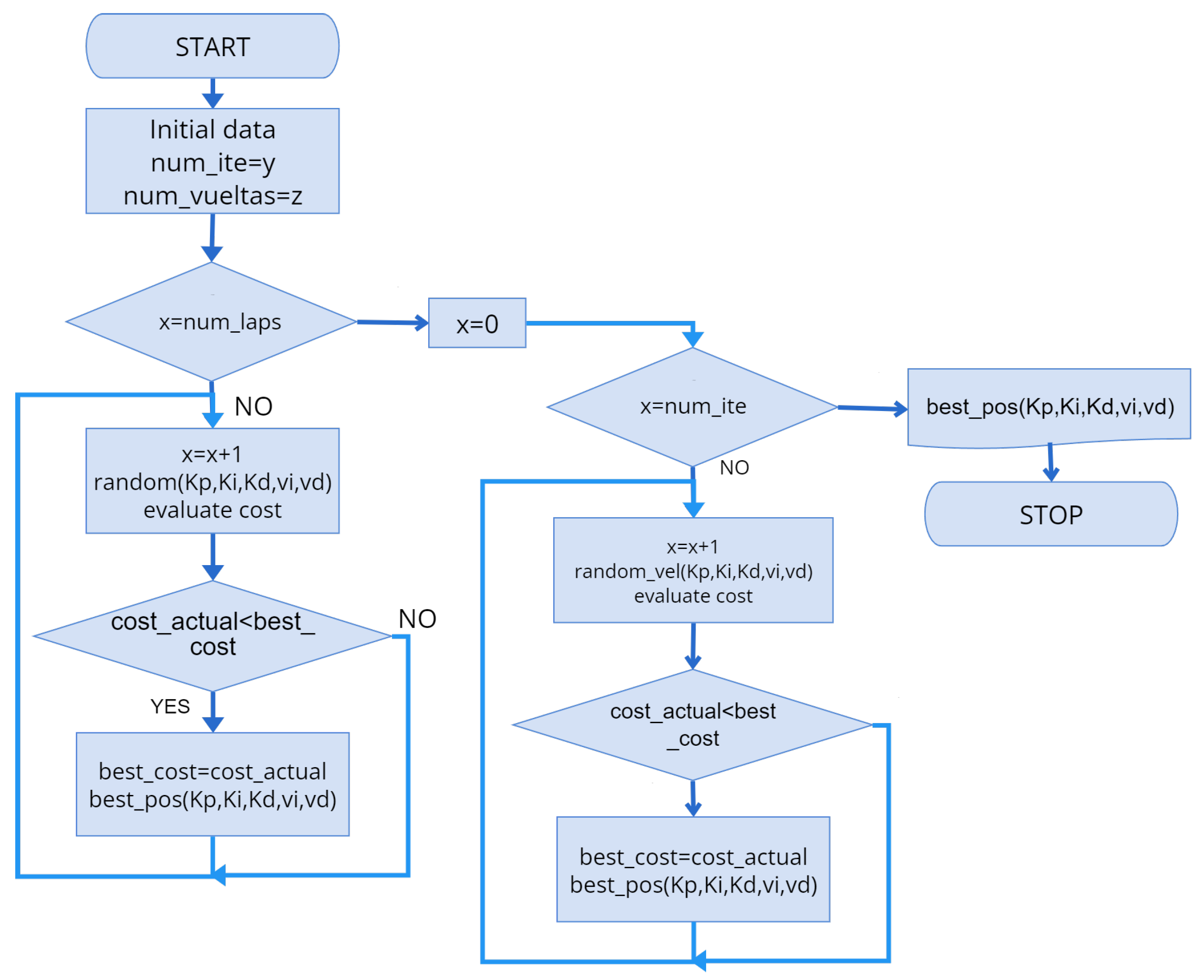
4.1. Controller Tuning

The particle swarm optimization (PSO) algorithm is briefly described in the theoretical framework shown in Figure 7. This procedure determines the best values of the gains of the different controllers.

Cost functions are widely used in the literature because they consider, in their structure, the different parameters or indexes that are to be minimized or maximized, as the case may be. In addition, they account for restrictions regarding the $\lambda$-dimensional search space. In order to quantify the best controller performance based on [62,63], among others, the objective function used in this work is given by

$$\begin{array}{c}\hfill OF=w_1{\int }_0^t\left|e\left(t\right)\right|dt+w_2{\int }_0^{t}t*\left|e\left(t\right)\right|dt\\ \hfill +w_3{\int }_0^{t}e{\left(t\right)}^{2}dt+w_4{\int }_0^{t}t*e{\left(t\right)}^{2}dt,\end{array}$$

(19)

where $e\left(t\right)=y\left(t\right)-r\left(t\right)$ is the control error. The elements in Equation (19) are derived from [62]. The first term, ${\int }_0^t\left|e\left(t\right)\right|dt$, represents the Integral Absolute Error. The second term, ${\int }_0^{t}t*\left|e\left(t\right)\right|dt$, corresponds to the Integral Time Absolute Error. The third term, ${\int }_0^{t}e{\left(t\right)}^{2}dt$, is the Integral Square Error, and the fourth term, ${\int }_0^{t}t*e{\left(t\right)}^{2}dt$, represents the Integral Time Square Error. The weights $w_1,w_2,w_3$ and $w_4$ assigned to these terms are based on the method described in [63], where a simplified version of PSO is employed, with maximum and minimum limits set for the weights. The weight factors $w_i$ establish the weighting of each index, depending on the scales or which one is given the greatest importance; for this function, the overpass or the stabilization time is not considered, because the problem in both cell banks and flotation columns lies in their oscillations and around the reference point more than how long it takes them to reach a stable state or the size of their overshoot.

When the gains of the integer and fractional PID controllers, $K_p$, $K_i$ and $K_d$, and the gains of the integer and fractional MRAC controller are within a range of $-100,100$ and the values of the fractional orders $\lambda$ and $\mu$ are within the range of $0,2$, simulation times will vary for both the flotation cell bank and the flotation column.

In particular, for the PSO method, the specific parameter values utilized in this study align with those defined in [64,65]:

• The initial population cannot be the same as the one chosen as in the literature, since up to three times as many parameters are optimized in our study. As the number of initial individuals is specific to each problem, in this study 150 particles were defined for the search process.
• The variable inertia factor was chosen to be $w_{max}=1.9$ and $w_{min}=0.4$.
• The acceleration constants were chosen to be $c_1=2$ and $c_2=2$.
• The maximum number of interactions was set as $ite{r}_{max}=1000$.

With these parameters and some variations for specific cases, and with $w_i=1$, the gains and fractional orders of the controllers were determined. Their corresponding simulation tests and an analysis of the results will be performed in the following section.

Therefore, it can be concluded that there are models of both the flotation cell bank and flotation column that are quite close to reality and ready for the development of controllers, with corresponding limitations. After this, the objective function was determined to determine the gains of the controllers in both plants.

The resultant parameters for the IOPI, FOPID, IOMRAC and FOMRAC controllers applied to the flotation cell bank and to the flotation column when there is a step change in the reference signal are shown in the table below.

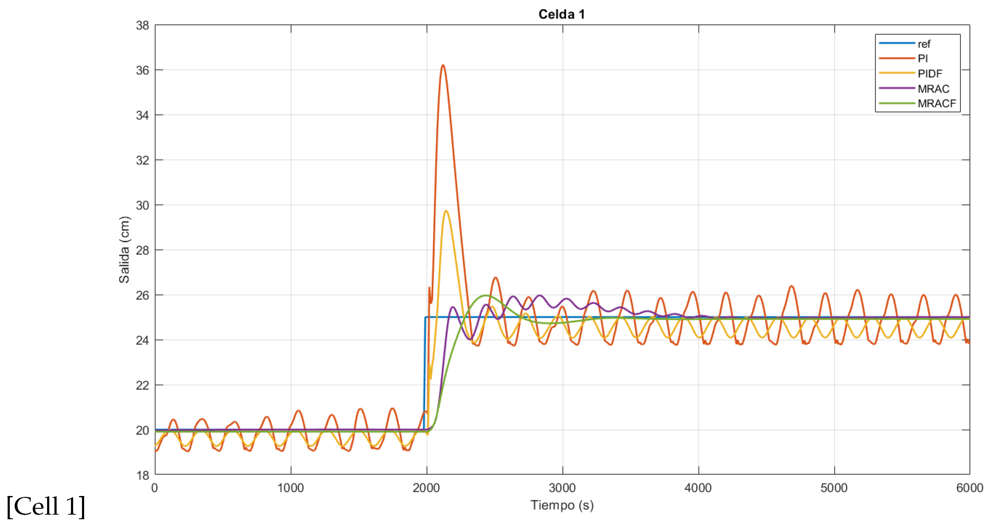
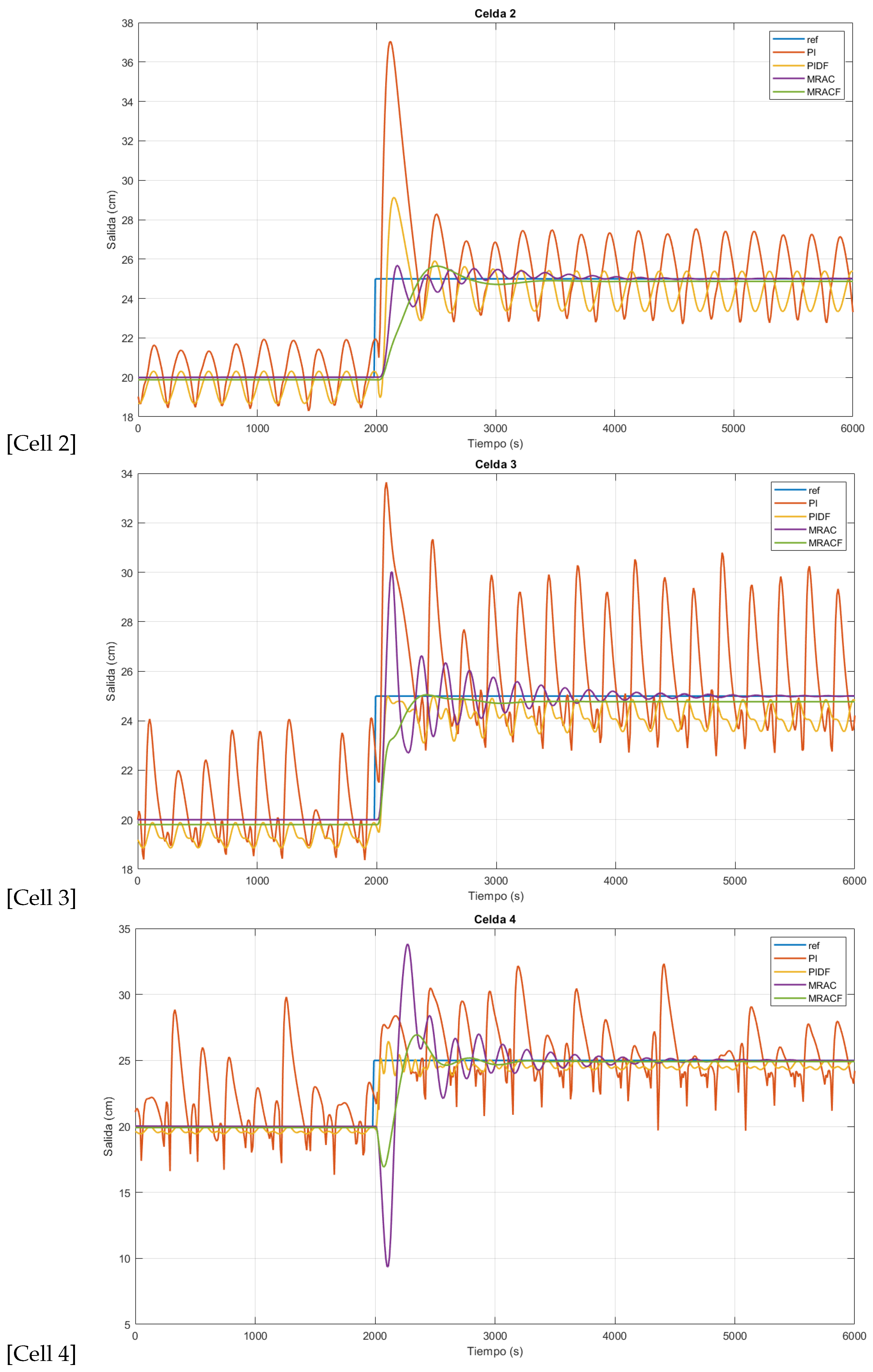
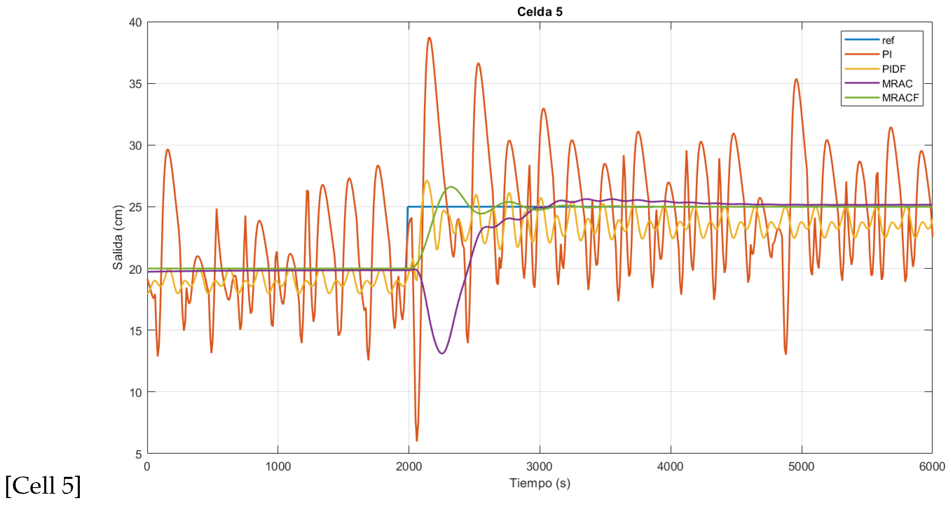
4.2. Flotation Cell Bank Behavior under Reference-Based Variations

For the flotation cell bank, a reference-based change from 20 to 25 cm was applied; these values are within the operating range and align with the point around which the mathematical model was identified. The simulation ran for 6000 s, with the reference’s change applied at 2000 s, similar to the tests performed in [34]. These reference-based changes are external inputs or adjustments made by technical supervisors, representing the real changes and values extracted from [34]. Physically, these changes correspond to maintaining a level close to the optimal extraction point of the valuable material. The control system regulates this level to ensure the efficient extraction of the target material during the flotation process. These reference-based changes are illustrated in Figure 8.

Table 2. Values and performance indexes with reference-based change from 20 to 25 cm.

	Controller	Gains	Mp (%)	${\mathit{t}}_{\mathit{r}}$ (s)	${\mathit{t}}_{\mathit{s}}$ (s)	ISE	ITSE	IAE	ITAE
Cell 1	IOPI	$K_p=24.99$	44.87	2020	∞	1.83 × 104	4.33 × 107	5599	1.62 × 107
		$K_i=0.0033$
	FOPID	$K_p=1.99$	18.93	2080	∞	4032	1.04 × 107	3090	9.06 × 106
		$K_i=2.17$
		$K_d=2.2$
		$\lambda =0.12$
		$\mu =0.26$
	IOMRAC	$\Gamma =0.0066$	3.86	2170	3270	2677	5.81 × 106	1327	3.43 × 106
	FOMRAC	$\Gamma =0.123$	3.84	2290	2580	2949	6.21 × 106	1488	3.67 × 106
		$\alpha =0.8$
Cell 2	IOPI	$K_p=24.99$	48.17	2040	∞	2.96 × 104	7.74 × 107	8858	2.65 × 107
		$K_i=0.0033$
	FOPID	$K_p=1.02$	16.5	2090	∞	8311	2.32 × 107	5137	1.54 × 107
		$K_i=0.9$
		$K_d=0.5$
		$\lambda =0.2$
		$\mu =0.04$
	IOMRAC	$\Gamma =6.35\times {10}^{-5}$	2.68	2150	2840	2289	4.81 × 106	1030	2.54 × 106
	FOMRAC	$\Gamma =0.104$	2.58	2370	2600	3619	7.68 × 106	1799	4.59 × 106
		$\alpha =0.543$
Cell 3	IOPI	$K_p=39.99$	34.56	2040	∞	3.28 × 104	1.04 × 108	1.03 × 104	3.24 × 107
		$K_i=0.0033$
	FOPID	$K_p=1.178$	0.032	2090	∞	5649	1.71 × 107	4784	1.48 × 107
		$K_i=1.9$
		$K_d=1.33$
		$\lambda =0.1$
		$\mu =0.08$
	IOMRAC	$\Gamma =0.757$	20.04	2080	3290	3356	7.44 × 106	1663	4.31 × 106
	FOMRAC	$\Gamma =0.742$	0.19	2370	2270	1921	4.25 × 106	1736	4.9 × 106
		$\alpha =0.318$
Cell 4	IOPI	$K_p=39.99$	29.29	2050	∞	4.3 × 104	1.03 × 108	1.2 × 104	3.23 × 107
		$K_i=0.0033$
	FOPID	$K_p=1.07$	5.84	2050	∞	1834	5.25 × 106	2565	7.86 × 106
		$K_i=2.4$
		$K_d=2.87$
		$\lambda =0.37$
		$\mu =0.1$
	IOMRAC	$\Gamma =0.04$	35.31	2190	3590	2.91 × 104	6.34 × 107	4181	1.02 × 107
	FOMRAC	$\Gamma =0.032$	7.75	2250	2480	8011	1.68 × 107	2075	4.93 × 106
		$\alpha =1.142$
Cell 5	IOPI	$K_p=39.99$	54.86	2110	∞	1.42 × 105	4 × 108	2.35 × 104	6.95 × 107
		$K_i=0.01533$
	FOPID	$K_p=1.6$	8.55	2100	∞	1.56 × 104	4.85 × 107	8191	2.54 × 107
		$K_i=2.07$
		$K_d=2.58$
		$\lambda =0.4$
		$\mu =0.29$
	IOMRAC	$\Gamma =4.06\times {10}^{-4}$	2.49	3060	3790	3.58 × 104	8.13 × 107	5704	1.42 × 107
	FOMRAC	$\Gamma =0.172$	6.47	2220	2590	2963	6.22 × 106	1105	2.51 × 106
		$\alpha =1.152$

Where $M_p$ is the maximum (percentage) overshoot; $t_r$ is the rise time, which is the time required for the response to go from $0\%$ to $100\%$ of its final value; and $t_s$ is the settling time, which is the time required for the response curve to reach its final value range (usually 2 or $5\%$), in this case $2\%$ was considered the final value. All this information was extracted from [66], and this applies to both the flotation cell bank and flotation column.

shows the gains from the PSO algorithm and the performance indexes according to the cells’ step response. The table details the control gains for each cell, including those using the IOPI, FOPID, IOMRAC, and FOMRAC. Specifically, it includes information on the proportional and integral gains of the IOPI, the fractional order and the gains of the FOPID, the adaptive law gains of the IOMRAC, and the fractional order of the FOMRAC.

It was observed that several controllers do not stabilize if their response is ∞; this is due to the constant oscillations maintained by their response that, being punctual, does not reach a stabilization time with the $2\%$ criterion.

In general and in most of the results, fractional controllers have an advantage over their integer counterparts, but, in general, in most performance indexes, the FOMRAC controller has an advantage over the others.

Figure 8 shows the behavior of cells when the reference is changed.

The most striking thing about the response in the first cell in Figure 8 is the 44.87% overshoot of the entire PI controller; it can be seen that both the IOPI and FOPID maintain constant oscillations, something that is solved by both the IOMRAC and FOMRAC.

In Figure 8, similarly to PI, cell 2 has a significant overshoot, in this case of 48.17%. Its oscillations are increased with respect to those of cell 1, which is true for both the IOPI and FOPID, and something totally solved by the IOMRAC and FOMRAC, in spite of the time the oscillations persist for, and this is not something that is attenuated.

It is observed that in cell 3 in Figure 8, the PI’s oscillations are similar to its overshoot and the IOMRAC shows oscillations that move closer to the reference point, while the FOPID reduces the amplitude of its oscillations with respect to cell 2 and both the IOMRAC and FOMRAC do not present oscillations after some simulation time.

In cell 4 in Figure 8, the PI’s results are very similar to those in the previous cell, where the oscillations are equal to or greater than the overshoot; in this case the FOPID reduces the oscillations even more, the IOMRAC presents a considerable negative overshoot, and only the FOMRAC eliminates the oscillations after a period of settling.

In cell 5, in Figure 8, oscillations equal to or greater than the previous cells are observed for the PI controller, while the FOPID manages to decrease the oscillations, the IOMRAC has a notable negative overshoot and the IOMRAC and FOMRAC both eliminate the oscillations.

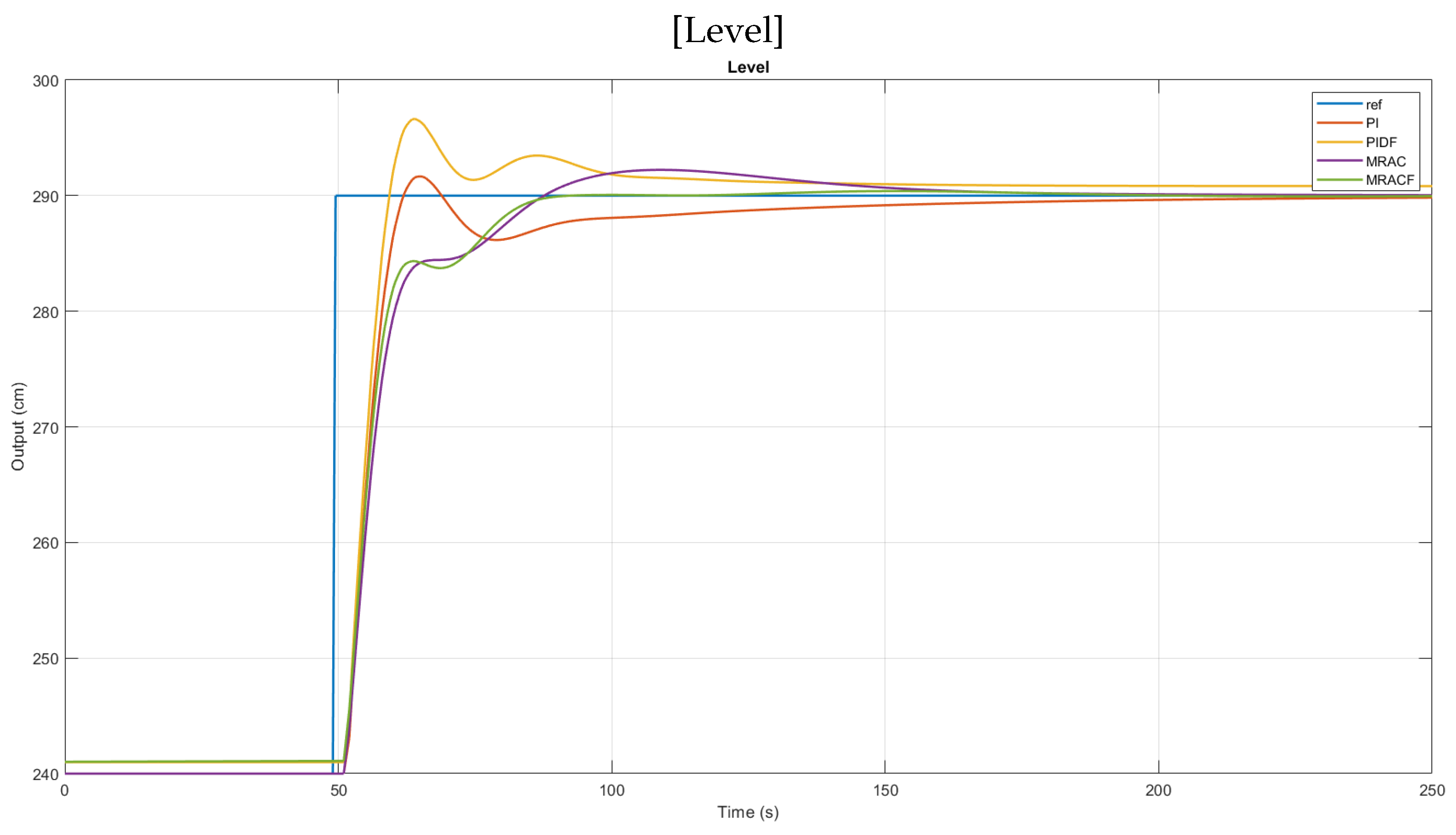
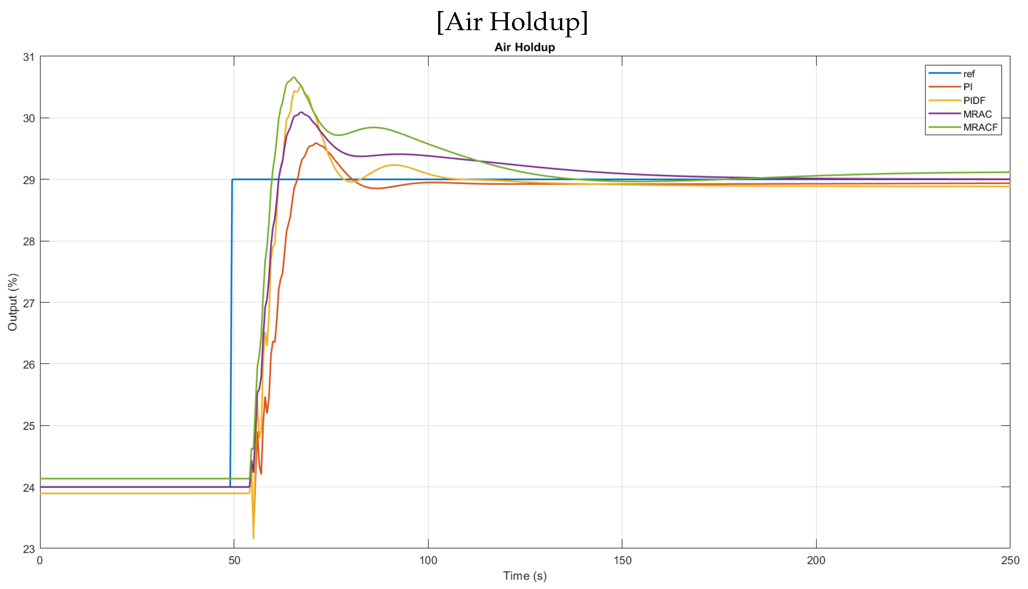
4.3. Flotation Column Behavior against Reference-Based Variations

For the flotation column, different reference-based changes were applied: a step change in the level (H) from 240 to 290 cm and a step change in the air holdup from 24% to 29%. The simulation lasted 250 s, with the referenced changes applied at 50 s, similar to the tests carried out in [30]. Since the column has a greater height, the values for its level are naturally higher. The specific process of column flotation allows for the control of additional variables; in this case, air holdup is considered, while other variables are kept constant. As with the flotation cell, the level changes are external references set by other programs or technical supervisors to ensure the optimal extraction of valuable material. The control of air holdup pertains to managing the air content within the column to maintain a stable flotation process performance, as in [30]. These reference-based changes are illustrated in Figure 9.

Table 3. Values and performance indexes with reference-based level change from 240 to 290 cm and air holdup change from 24 to 29%.

	Controller	Gains	${\mathit{M}}_{\mathit{p}}$ (%)	${\mathit{t}}_{\mathit{r}}$ (s)	${\mathit{t}}_{\mathit{s}}$ (s)	ISE	ITSE	IAE	ITAE
Level	IOPI	$K_p=-6.79$	0.75	62	139.5	1101	5.85 × 104	144.9	9797
		$K_i=-0.05$
	FOPID	$K_p=-8.98$	2.29	59.5	148.5	1046	5.75 × 104	190.8	16,530
		$K_i=-0.92$
		$K_d=4.118$
		$\lambda =0.726$
		$\mu =0.15$
	IOMRAC	${\Gamma }_1=0.09$	0.76	88	141	1328	7.25 × 104	180.4	13,180
		${\Gamma }_2=2.14$
	FOMRAC	${\Gamma }_1=0.32$	0.13	92.5	83	1169	6.24 × 104	156.6	9302
		${\Gamma }_2=2.9$
		${\alpha }_1=1.25$
		${\alpha }_2=0.94$
Air Holdup	IOPI	$K_p=-140.41$	2.04	67	78	2721	1.53 × 105	288	2.48 × 104
		$K_i=0.52$
	FOPID	$K_p=160.55$	5.2	54.5	99.5	2367	1.32 × 105	261.3	2.07 × 104
		$K_i=6.73$
		$K_d=15.92$
		$\lambda =0.873$
		$\mu =0.13$
	IOMRAC	${\Gamma }_1=3.72$	3.77	61.5	148.5	2068	1.16 × 105	248.7	1.87 × 104
		${\Gamma }_2=0.46$
	FOMRAC	${\Gamma }_1=0.32$	5.74	60	126	2113	1.24 × 105	312.7	2.43 × 104
		${\Gamma }_2=0.16$
		${\alpha }_1=0.54$
		${\alpha }_2=1.43$

shows the gains from the PSO algorithm and the performance indexes of the controllers according to the step response of the flotation column. The table details the control gains for column flotation, including when using the IOPI, FOPID, IOMRAC and FOMRAC. Specifically, it provides information on the proportional and integral gains of the IOPI, the fractional order and associated gains of the FOPID, the adaptive law gains of the IOMRAC, and the fractional order of the FOMRAC.

It can be seen that, in terms of level control, the FOMRAC controller has an advantage in terms of overshoot; in terms of rise time ($t_r$), the FOPID controller responds best; in terms of settling time ($t_s$), the FOMRAC controller has a clear advantage, as shown in Figure 9.

While in Figure 9 it can be observed that there is no marked difference in the controllers in the case of the flotation cell bank, Table 3 quantitatively details the advantages of fractional controllers over integer-based ones. Although small in proportion, this advantage can be highlighted in the output curve corresponding to the FOMRAC controller, which arrives smoothly at the control level.

In Table 3, in terms of air holdup control, it can be observed that, in terms of the percentage of overpass, the PI controller has better results, while, for the rise time, the FOPID controller has an advantage and, in terms of other indicators, the FOPID controller has better results. This is graphically evidenced in Figure 9.

It is observed that all the controllers reach a steady state, with the FOPID controller having a slight advantage over the others here and in its rise time. Generally, in most performance indexes, fractional controllers have an advantage, with a few exceptions.

In conclusion, after designing IOPI, FOPID, IOMRAC and FOMRAC controllers for a flotation cell bank and a flotation column, their simulation show adequate results; in all cases the error is eliminated asymptotically, except for in the flotation cell bank with a PI controller, which is the same problem exhibited in [34].

Comparative evaluations of the controllers were carried out in both plants, in different scenarios and with the proposed performance indexes; the results are quantitatively presented in Table 2 and Table 3, with different controllers having advantages in different indexes, but, in general, the fractional controllers having the advantage.

5. Conclusions

Starting with our motivation to study the topic presented, the application of fractional calculus concepts to control systems was proposed as our objective. In this sense, this work allows us to conceptualize the fact that fractional calculus presents viable and interesting alternatives that can be applied to engineering processes, particularly in automation, through the extension of control schemes that traditionally use integer-order integration and derivation to the those of fractional orders, whether in terms of integration, derivation or both.

It is concluded that these mathematical models respond in a way that is very similar to a real flotation cell bank and a real flotation column. Therefore, it is inferred that the results of these simulations could be considered suitable for direct implementation, with the corresponding adaptation of both sensors and actuators.

The level and air holdup variables affecting the efficiency of the process were selected as control targets. In this research, the other variables were considered constant. IOPID, IOMRAC, FOPID and FOMRAC controllers were designed using the PSO algorithm and simulated. Regarding the interaction between system variables, the performance of the IOPID control loop was not desirable, especially in the flotation cell bank. In the flotation cells, the FOMRAC controller in particular exhibited almost no oscillations, while all other controllers showed characteristic process oscillations. Comparing the IOPID with the FOPID, the fractional controller significantly reduced these oscillations. Considering level control in the flotation column, the IOPID and FOPID exhibited notable overshoot, with the FOPID showing a lower overshoot. However, the FOMRAC did not exhibit this overshoot, indicating its superior performance. The performance of the FOPID and FOMRAC were better in terms of the ISE, ITSE, IAE and ITAE indices.

This suggests that the integer controllers used for some industrial flotation processes could be replaced by fractional controllers, which are of low cost and low implementation complexity compared to MPC controllers and result in a better performance than integer controllers.

A significant limitation of this work lies in its simulation aspect, even though the models used are based on real processes. Another limitation is that fractional calculus requires more processing capacity. It is important to address the discretization of fractional calculus and controllers for their implementation outside of MATLAB, such as in microcontrollers or systems with only discrete programming, which could be a direction for future work.

Our future work will include real-world experimentation with fractional controllers, either through their practical implementation in industrial settings or through controlled laboratory experiments. Additionally, efforts will be made to explore a discretization design for fractional calculus, enhancing the applicability of these controllers in digital systems. Other optimization techniques beyond PSO will be investigated for adaptive controllers, with a particular focus on methods that do not rely on specific models, leveraging the inherent flexibility of adaptive control strategies. Comparisons will be made between various fractional controllers and different adaptive configurations to assess their relative performances. Furthermore, future research will address the process as a nonlinear system, moving beyond the viewpoint of operation around a single point. It is also essential to explore alternative methods for calculating fractional calculus, such as fractional dimensional reproducing kernel spaces [2], to fully capitalize on the benefits of these advanced techniques.

In brief, fractional controllers demonstrate superior behavior compared to integer controllers, requiring minimal changes in their design or implementation but necessitating greater computational processing.

References

1. Oldham, K.; Spanier, J. The Fractional Calculus Theory and Applications of Differentiation and Integration to Arbitrary Order; Elsevier Science: Amsterdam, The Netherlands, 1974; pp. 1–322. [Google Scholar]
2. Li, Z.; Chen, Q.; Wang, Y.; Li, X. Solving Two-Sided Fractional Super-Diffusive Partial Differential Equations with Variable Coefficients in a Class of New Reproducing Kernel Spaces. Fractal Fract. 2022, 6, 492. [Google Scholar] [CrossRef]
3. Duarte-Mermoud, M.A.; Aguila-Camacho, N.; Gallegos, J.A.; Travieso-Torres, J.C. Fractional-order model reference adaptive controllers for first-order integer plants. In New Perspectives and Applications of Modern Control Theory: In Honor of Alexander S. Poznyak; Springer: Cham, Switzerland, 2018; pp. 121–151. [Google Scholar]
4. Aguila-Camacho, N.; García-Bustos, J.E.; Castillo-López, E.I.; Gallegos, J.A.; Travieso-Torres, J.C. Switched Fractional Order Model Reference Adaptive Control for First Order Plants: A Simulation-Based Study. J. Dyn. Syst. Meas. Control 2022, 144, 044502. [Google Scholar] [CrossRef]
5. Fuerstenau, M.C.; Han, K.N. Principles of Mineral Processing; SME: Littleton, CO, USA, 2003. [Google Scholar]
6. Vinagre, B.M.; Monje, C.A. Introduccion al control fraccionario. Rev. Iberoam. Autom. Inform. Ind. 2006, 3, 5–23. [Google Scholar]
7. Thivierge, A.; Bouchard, J.; Desbiens, A. Economic model predictive control of a high-pressure grinding rolls circuit: Energy considerations. IFAC-PapersOnLine 2022, 55, 55–60. [Google Scholar] [CrossRef]
8. Vinagre, B.M.; Monje, C.A. Fractional PID Controllers for Industry Application. A Brief Introduction. J. Vib. Control 2007, 13, 1419–1429. [Google Scholar] [CrossRef]
9. Fujii, S.; Mizuno, N. Multivariable Discrete Model Reference Adaptive Control Using an Autoregressive Model with Dead Time of the Plant and Its Application. Trans. Soc. Instrum. Control Eng. 1982, 18, 238–245. [Google Scholar] [CrossRef]
10. Elliott, H.; Wolovich, W. A parameter adaptive control structure for linear multivariable systems. IEEE Trans. Autom. Control 1982, 27, 340–352. [Google Scholar] [CrossRef]
11. Quintanilla, P.; Navia, D.; Neethling, S.J.; Brito-Parada, P.R. Economic model predictive control for a rougher froth flotation cell using physics-based models. Miner. Eng. 2023, 196, 108050. [Google Scholar] [CrossRef]
12. Anzoom, S.J.; Bournival, G.; Ata, S. Coarse particle flotation: A review. Miner. Eng. 2024, 206, 108499. [Google Scholar] [CrossRef]
13. Azhin, M.; Popli, K.; Prasad, V. Modelling and boundary optimal control design of hybrid column flotation. Can. J. Chem. Eng. 2021, 99, S369–S388. [Google Scholar] [CrossRef]
14. Xu, X.; Tian, Y.; Yuan, Y.; Luan, X.; Liu, F.; Dubljevic, S. Output regulation of linearized column froth flotation process. IEEE Trans. Control Syst. Technol. 2020, 29, 249–262. [Google Scholar] [CrossRef]
15. Chen, J.; Chimonyo, W.; Peng, Y. Flotation behaviour in reflux flotation cell–A critical review. Miner. Eng. 2022, 181, 107519. [Google Scholar] [CrossRef]
16. Quintanilla, P.; Neethling, S.J.; Navia, D.; Brito-Parada, P.R. A dynamic flotation model for predictive control incorporating froth physics. Part I: Model development. Miner. Eng. 2021, 173, 107192. [Google Scholar] [CrossRef]
17. Quintanilla, P.; Neethling, S.J.; Mesa, D.; Navia, D.; Brito-Parada, P.R. A dynamic flotation model for predictive control incorporating froth physics. Part II: Model calibration and validation. Miner. Eng. 2021, 173, 107190. [Google Scholar] [CrossRef]
18. Norlund, F. Comparison of Level Control Strategies for a Flotation Series in the Mining Industry. Master’s Thesis, Lund University, Lund, Sweden, 2022. [Google Scholar]
19. Yianatos, J.; Vallejos, P.; Grau, R.; Yañez, A. New approach for flotation process modelling and simulation. Miner. Eng. 2020, 156, 106482. [Google Scholar] [CrossRef]
20. Yianatos, J.; Vallejos, P. Limiting conditions in large flotation cells: Froth recovery and bubble loading. Miner. Eng. 2022, 185, 107695. [Google Scholar] [CrossRef]
21. Jera, T.M.; Bhondayi, C. A review on froth washing in flotation. Minerals 2022, 12, 1462. [Google Scholar] [CrossRef]
22. Quintanilla, P.; Navia, D.; Neethling, S.; Brito-Parada, P. Experimental Implementation of an Economic Model Predictive Control for Froth Flotation. In Computer Aided Chemical Engineering; Elsevier: Amsterdam, The Netherlands, 2024; Volume 53, pp. 1759–1764. [Google Scholar]
23. Sun, B.; Yang, W.; He, M.; Wang, X. An integrated multi-mode model of froth flotation cell based on fusion of flotation kinetics and froth image features. Miner. Eng. 2021, 172, 107169. [Google Scholar] [CrossRef]
24. Nasseri, S.; Khalesi, M.R.; Ramezani, A.; Abdollahi, M.; Mohseni, M. An Adaptive Decoupling Control Design for Flotation Column: A Comparative Study Against Model Predictive Control. IETE J. Res. 2022, 68, 3994–4007. [Google Scholar] [CrossRef]
25. Maldonado, M.; Desbiens, A.; Del Villar, R. Potential use of model predictive control for optimizing the column flotation process. Int. J. Miner. Process. 2009, 93, 26–33. [Google Scholar] [CrossRef]
26. Tian, Y.; Luan, X.; Liu, F.; Dubljevic, S. Model predictive control of mineral column flotation process. Mathematics 2018, 6, 100. [Google Scholar] [CrossRef]
27. Calisaya, D.; Poulin, É.; Desbiens, A.; del Villar, R.; Riquelme, A. Multivariable predictive control of a pilot flotation column. In Proceedings of the 2012 American Control Conference (ACC), Montreal, QC, Canada, 27–29 June 2012; pp. 4022–4027. [Google Scholar]
28. Mohanty, S. Artificial neural network based system identification and model predictive control of a flotation column. J. Process Control 2009, 19, 991–999. [Google Scholar] [CrossRef]
29. Riquelme, A.; Desbiens, A.; Del Villar, R.; Maldonado, M. Predictive control of the bubble size distribution in a two-phase pilot flotation column. Miner. Eng. 2016, 89, 71–76. [Google Scholar] [CrossRef]
30. Ccarita-Cruz, J.C. Diseño de un Controlador Predictivo Generalizado Multivariable para el Control de una Celda de Flotación tipo Columna Utilizada en el Proceso de Recuperación de Cobre. Master’s Thesis, Pontifica Universidad Católica del Perú, San Miguel, Peru, 2017. [Google Scholar]
31. Quintanilla, P.; Neethling, S.J.; Brito-Parada, P.R. Modelling for froth flotation control: A review. Miner. Eng. 2021, 162, 106718. [Google Scholar] [CrossRef]
32. Jovanović, I.; Miljanović, I. Contemporary advanced control techniques for flotation plants with mechanical flotation cells–A review. Miner. Eng. 2015, 70, 228–249. [Google Scholar] [CrossRef]
33. Putz, E.; Cipriano, A. Hybrid model predictive control for flotation plants. Miner. Eng. 2015, 70, 26–35. [Google Scholar] [CrossRef]
34. Troncoso-Garay, C.E. Diseño e implementación de estrategia de control predictivo en proceso de flotación de minerales. Master’s Thesis, Universidad Técnica Federico Santa María, Valparaíso, Chile, 2016. [Google Scholar]
35. Duarte-Mermoud, M.A. Advances in Fractional Control. In Proceedings of the CHILEAN Conference on Electrical, Electronics Engineering, Information and Communication Technologies, Santiago, Chile, 28–30 October 2015; pp. 413–415. [Google Scholar]
36. Jauregui, C.; Duarte-Mermoud, M.; Orostica, R. Conical Tank Level Control with Fractional PID. IEEE Lat. Am. Trans. 2016, 14, 2598–2604. [Google Scholar] [CrossRef]
37. Bürger, R.; Diehl, S.; Martí, M.C.; Vásquez, Y. Simulation and control of dissolved air flotation and column froth flotation with simultaneous sedimentation. Water Sci. Technol. 2020, 81, 1723–1732. [Google Scholar] [CrossRef]
38. Wepener, D.; le Roux, J.; Craig, I. Disturbance Propagation Through a Grinding-Flotation Circuit. IFAC-PapersOnLine 2021, 54, 19–24. [Google Scholar] [CrossRef]
39. Le Roux, J.D.; Craig, I.K. Plant-wide control framework for a grinding mill circuit. Ind. Eng. Chem. Res. 2019, 58, 11585–11600. [Google Scholar] [CrossRef]
40. Jämsä-Jounela, S.L.; Dietrich, M.; Halmevaara, K.; Tiili, O. Control of pulp levels in flotation cells. Control Eng. Pract. 2003, 11, 73–81. [Google Scholar] [CrossRef]
41. Podlubny, I. Fractional Differential Equations: An Introduction to Fractional Derivatives, Fractional Differential Equations, to Methods of Their Solution and Some of Their Applications; Elsevier: Amsterdam, The Netherlands, 1998; pp. 1–337. [Google Scholar]
42. Miller, K.S.; Ross, B. An Introduction to the Fractional Calculus and Fractional Differential Equations, Ilustrada ed.; Wiley: Hoboken, NJ, USA, 1993; pp. 1–384. [Google Scholar]
43. Kilbas, A.; Srivastava, H.; Trujillo, J. Theory and Applications of Fractional Differential Equations, 1st ed.; van Mill, J., Ed.; Elsevier: Amsterdam, The Netherlands, 2006; pp. 1–523. [Google Scholar]
44. Pan, I.; Das, S. Intelligent Fractional Order Systems and Control; Springer: Berlin/Heidelberg, Germany, 2013; pp. 1–298. [Google Scholar]
45. Nanendra, K.S.; Annaswamy, A.M. Stable Adaptive Systems, 5th ed.; Dover Publications: Mineola, NY, USA, 2005; pp. 1–512. [Google Scholar]
46. El-Khazali, R. Fractional-order PID (fractional) controller design. Comput. Math. Appl. 2013, 66, 639–646. [Google Scholar] [CrossRef]
47. Ostalczyk, P. Stability analysis of a discrete-time system with a variable, fractional-order controller. Inst. Autom. 2010, 58, 613–619. [Google Scholar] [CrossRef]
48. Vinagre, B.M.; Feliu-Batlleb, V.; Tejadoa, I. Control fraccionario: Fundamentos y guia de uso. Rev. Iberoam. Automát. Informát. Ind. 2016, 13, 265–280. [Google Scholar] [CrossRef]
49. Sagayaraj, M.R.; Selvam, A.G.M. Discrete fractional calculus: Definitions and applications. Int. J. Pure Eng. Math. 2014, 2, 93–102. [Google Scholar]
50. Dzieliński, A.; Sierociuk, D.; Sarwas, G. Some applications of fractional order calculus. Bull. Pol. Acad. Sci. 2010, 58, 583–592. [Google Scholar] [CrossRef]
51. Guo, J.; Liu, Y.; Tao, G. Multivariable MRAC with state feedback for output tracking. In Proceedings of the 2009 American Control Conference, St. Louis, MO, USA, 10–12 June 2009; pp. 592–597. [Google Scholar]
52. Tao, G. Model reference adaptive control of multivariable plants with delays. Int. J. Control. 1992, 55, 393–414. [Google Scholar] [CrossRef]
53. Das, M. Multivariable Adaptive Model Matching Using Less A Priori Information. J. Dyn. Syst. Meas. Control 1986, 108, 151–153. [Google Scholar] [CrossRef]
54. Guo, J.; Tao, G.; Liu, Y. A multivariable MRAC scheme with application to a nonlinear aircraft model. Automatica 2011, 47, 804–812. [Google Scholar] [CrossRef]
55. Guo, J.; Tao, G. A discrete-time multivariable MRAC scheme applied to a nonlinear aircraft model with structural damage. Automatica 2015, 53, 43–52. [Google Scholar] [CrossRef]
56. Hsu, L.; Minhoto-Teixeira, M.C.; Costa, R.R. Lyapunov design of multivariable MRAC via generalized passivation. Asian J. Control 2015, 17, 1484–1497. [Google Scholar] [CrossRef]
57. Lazo-Berrezueta, A.A. Implementación de un Controlador Adaptativo por Modelo de Referencia para Sistemas de Segundo Orden. Master’s Thesis, Universidad Politecnica Salesiana Ecuador, Cuenca, Ecuador, 2016. [Google Scholar]
58. Duarte-Mermoud, M.A.; Aguila-Camacho, N.; Gallegos, J.A.; Castro-Linares, R. Using general quadratic Lyapunov functions to prove Lyapunov uniform stability for fractional order systems. Commun. Nonlinear Sci. Numer. Simul. 2015, 22, 650–659. [Google Scholar] [CrossRef]
59. Sutulov, A. Flotación de Minerales; Universidad de Concepción, Instituto de Investigaciones Tecnológicas: Concepción, Chile, 1963; pp. 1–331. [Google Scholar]
60. Salager, G. Fundamentos de La Flotación de Minerales; Universidad de los Andes: Bogotá, Colombia, 2007; pp. 1–21. [Google Scholar]
61. Cruz, E.B. Simulation of Computer Control Strategies for Column Flotation. Master’s Thesis, Virginia Tech, Blacksburg, VA, USA, 1994. [Google Scholar]
62. Rasool, H.; Rasool, A.; Ikram, A.A.; Rasool, U.; Jamil, M. Compatibility of objective functions with simplex algorithm for controller tuning of HVDC system. Ing. E Investig. 2019, 39, 34–43. [Google Scholar] [CrossRef]
63. Panda, S.; Sahu, B.K.; Mohanty, P.K. Design and performance analysis of PID controller for an automatic voltage regulator system using simplified particle swarm optimization. J. Frankl. Inst. 2012, 349, 2609–2625. [Google Scholar] [CrossRef]
64. Ortiz-Quisbert, M.; Duarte-Mermoud, M.; Milla, F.; Castro-Linares, R. Control Adaptativo Fraccionario Optimizado por Algoritmos Genéticos, Aplicado a Reguladores Automáticos de Voltaje. Rev. Iberoam. De Automát. Informát. Ind. RIAI 2016, 13, 403–409. [Google Scholar] [CrossRef]
65. Chatterjee, A.; Mukherjee, V.; Ghoshal, S.P. Velocity relaxed and craziness-based swarm optimized intelligent PID and PSS controlled AVR system. Int. J. Electr. Power Energy Syst. 2009, 31, 323–333. [Google Scholar] [CrossRef]
66. Ogata, K. Ingenieria de Control Moderna; Pearson: London, UK, 2010; pp. 1–965. [Google Scholar]
Figure 1. Diagram of the PI system.
Mathematics 12 02789 g001
Figure 2. Schematic representation of the fractional-order PID controller compared to its integer-order counterpart [44].
Mathematics 12 02789 g002
Figure 3. Diagram of the MRAC used in the system.
Mathematics 12 02789 g003
Figure 4. Operating principle of flotation cell process.
Mathematics 12 02789 g004
Figure 5. Configuration of a flotation cell bank.
Mathematics 12 02789 g005
Figure 6. Schematic diagram of the flotation column.
Mathematics 12 02789 g006
Figure 7. PSO flowchart.
Mathematics 12 02789 g007
Figure 8. Response of the cells to a step change from 20 to 25 cm.
Mathematics 12 02789 g008aMathematics 12 02789 g008bMathematics 12 02789 g008c
Figure 9. Float column level with reference-based changes.
Mathematics 12 02789 g009aMathematics 12 02789 g009b