
Fuzzy Optimization Model for Decision-Making in Single Machine Construction Project Planning


 , ,
, ,  , and
, and
Abstract
1. Introduction
2. Materials and Methods
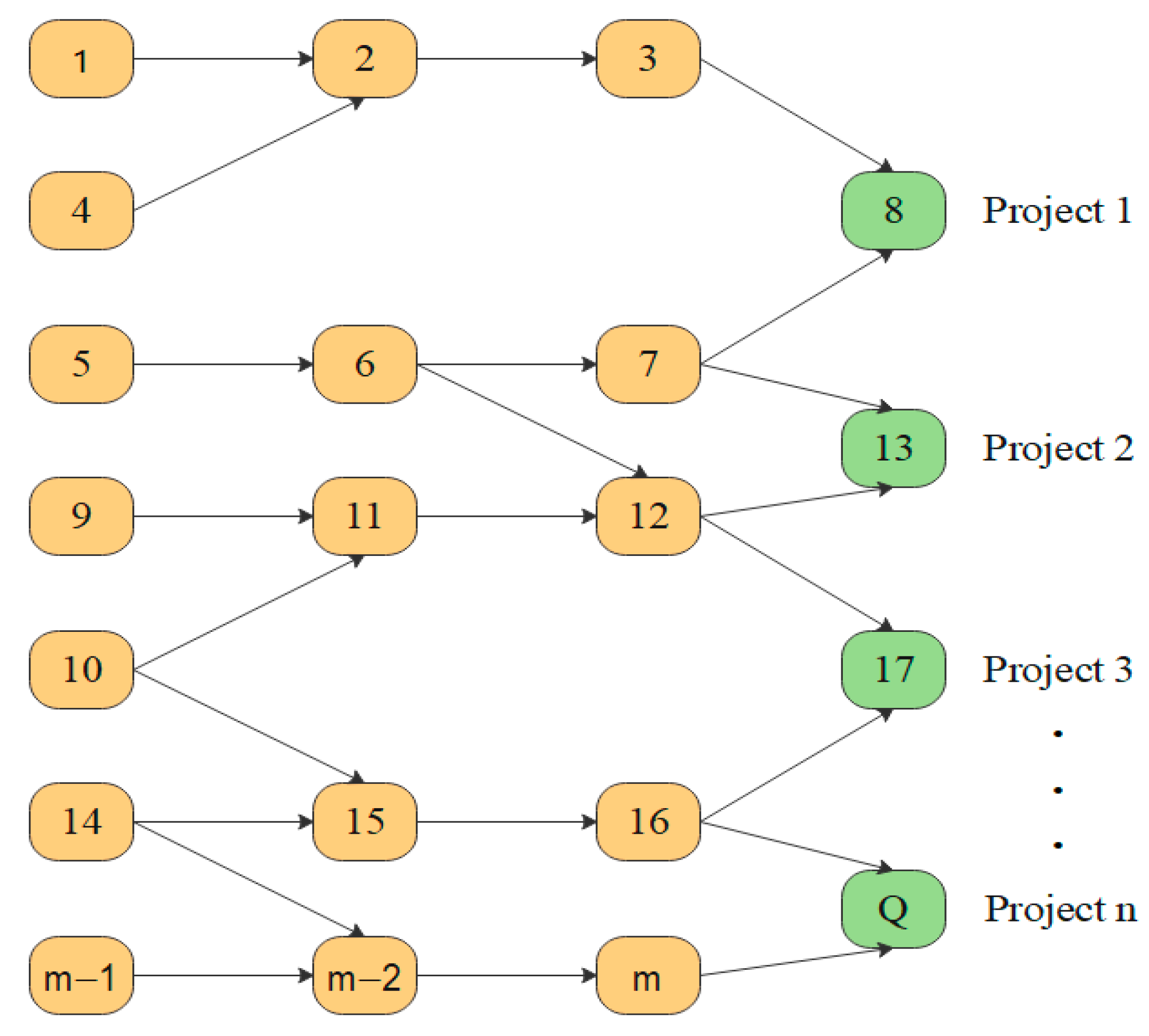
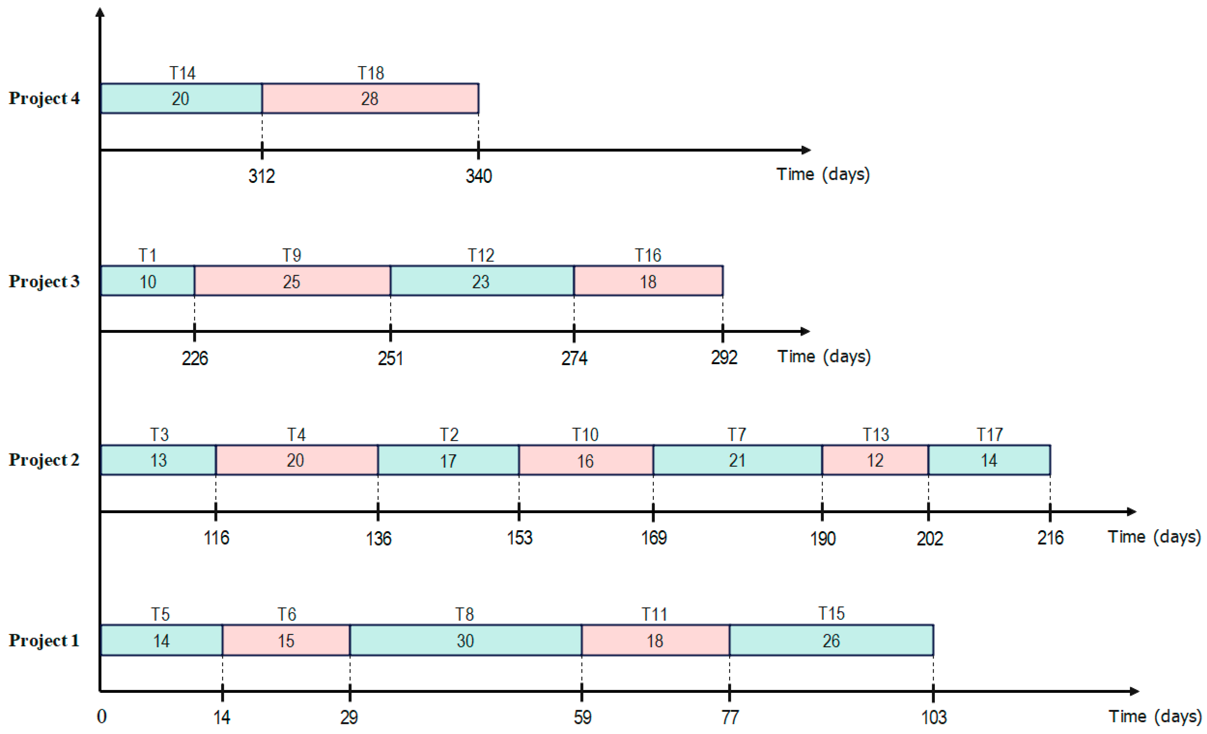
2.1. Scheduling of Single-Machine Construction Projects
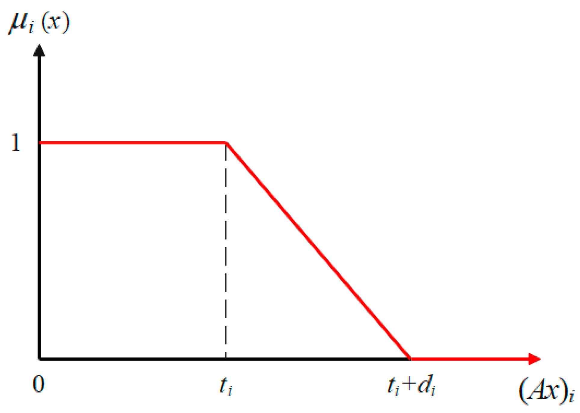
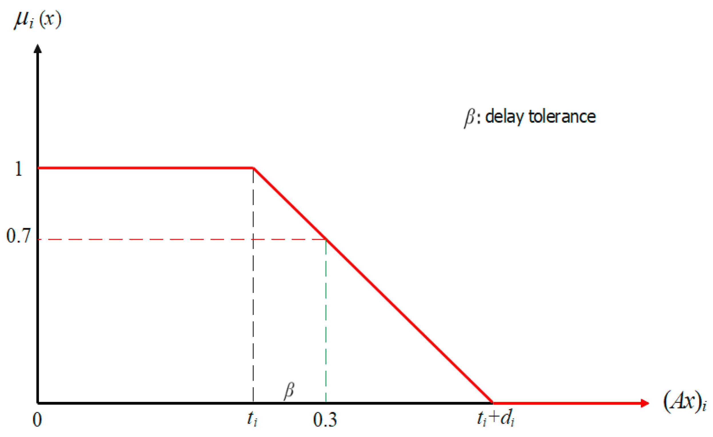
2.2. Fuzzy Sets
2.3. Linear Programming with Fuzzy Resources
2.4. Verdegay Method
2.5. A Fuzzy Optimization Model for Single-Machine Construction Projects Scheduling
2.6. Solution of the Proposed Model
| Algorithm 1. Mixed Integer Linear Programming model | |
| Input: Set of “T” tasks to perform a set of “P” projects Output: Scheduling of tasks for the realization of “P” projects For each | |
| (14) | |
| subject to: | |
| (15) | |
| (16) | |
| (17) | |
| (18) | |
|
where: |
3. Results
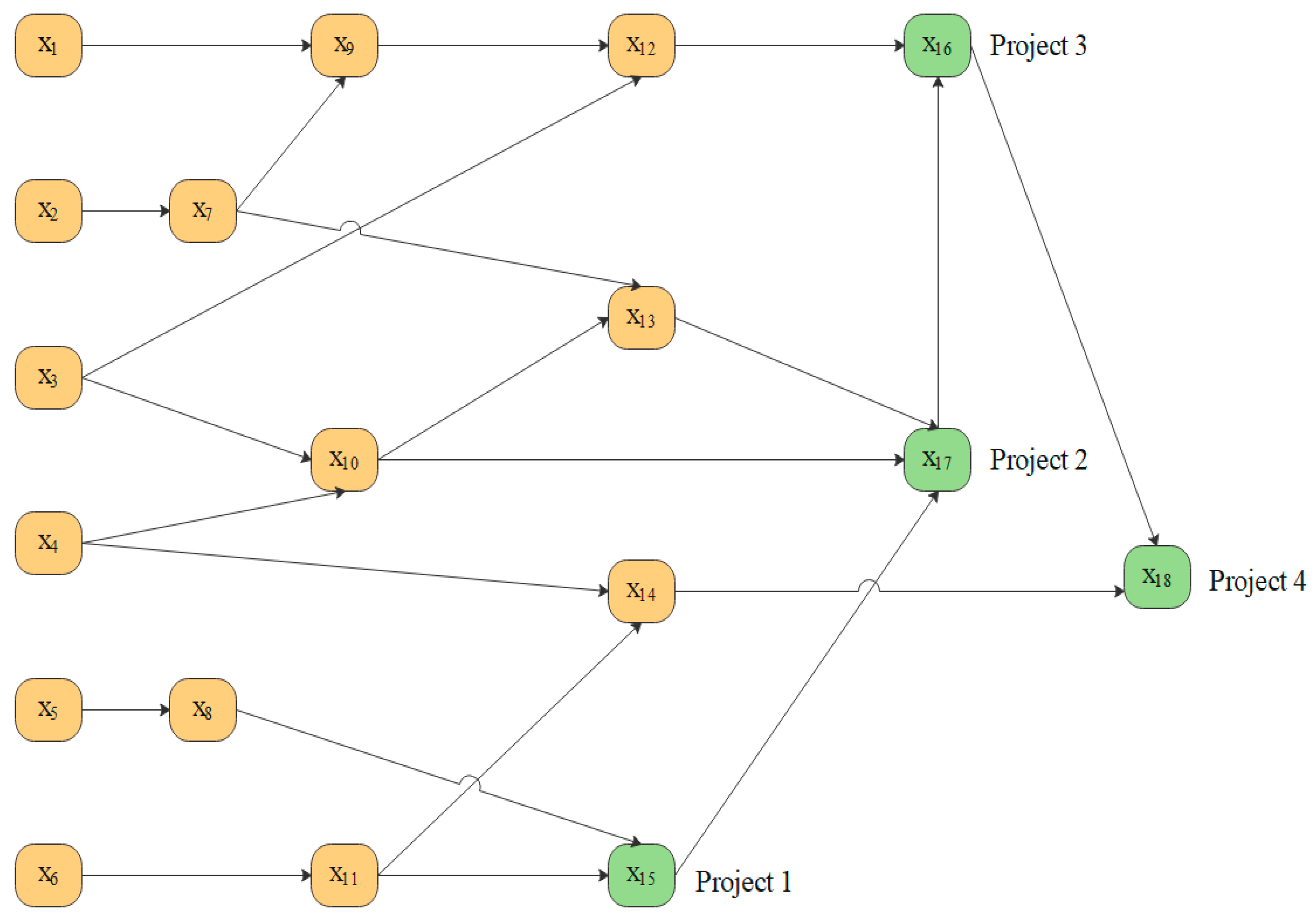
3.1. Case Study
3.2. Case Study Evaluation
3.3. Application of Fuzzy Model
- Step 1:
- Managers should review their portfolios of pending construction projects.
- Step 2:
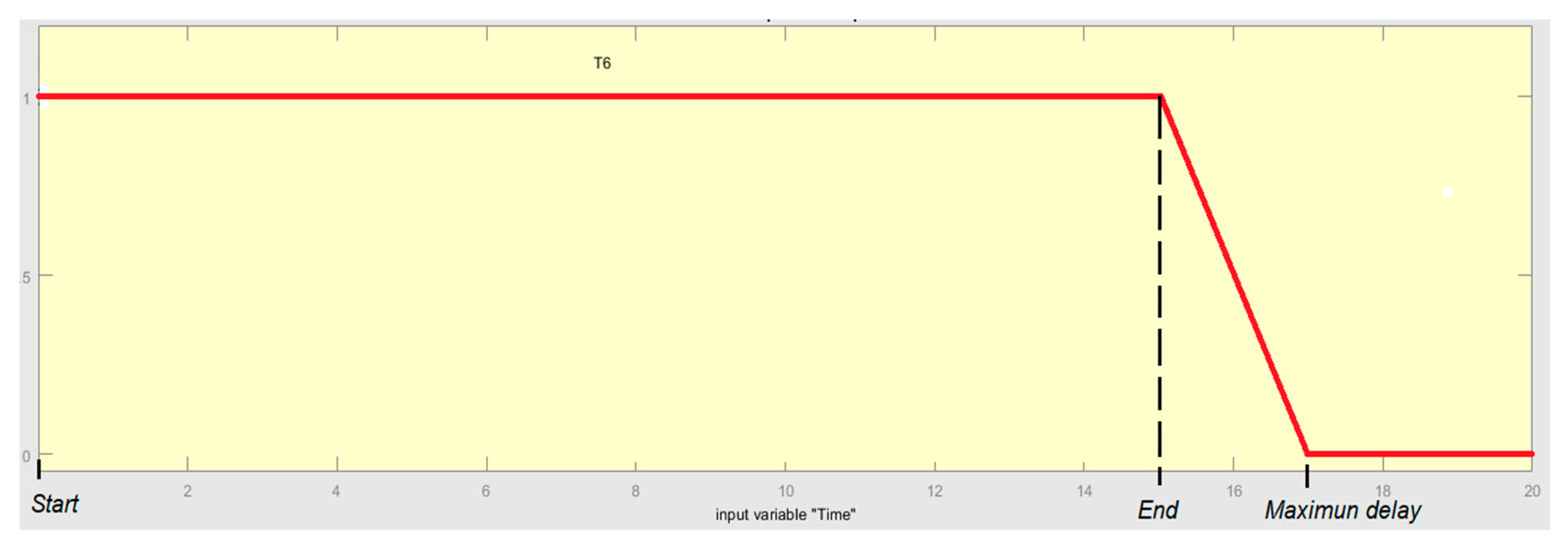
- Experts in the execution of construction projects must create a table indicating, for each task, the start time, processing time, and maximum tolerance time for the machine to complete the task. The experts should also indicate the degree of imprecision in the delays (), which can be tolerated for all tasks.
- Step 3:
- With the data from Step 2, the rectangular triangular fuzzy set representing the maximum delay to be tolerated must be designed for each task.
- Step 4:
- Enter the parameters required by the model: for each task, enter the start time and the fuzzy set representing the processing time, the degree of delay tolerated for all tasks, the delivery time for each project, and the penalty for each day of delay.
- Step 5:
- Solve the MILP auxiliary model using a linear programming solver. The decision variables obtained are (start of task ).
- Step 6:
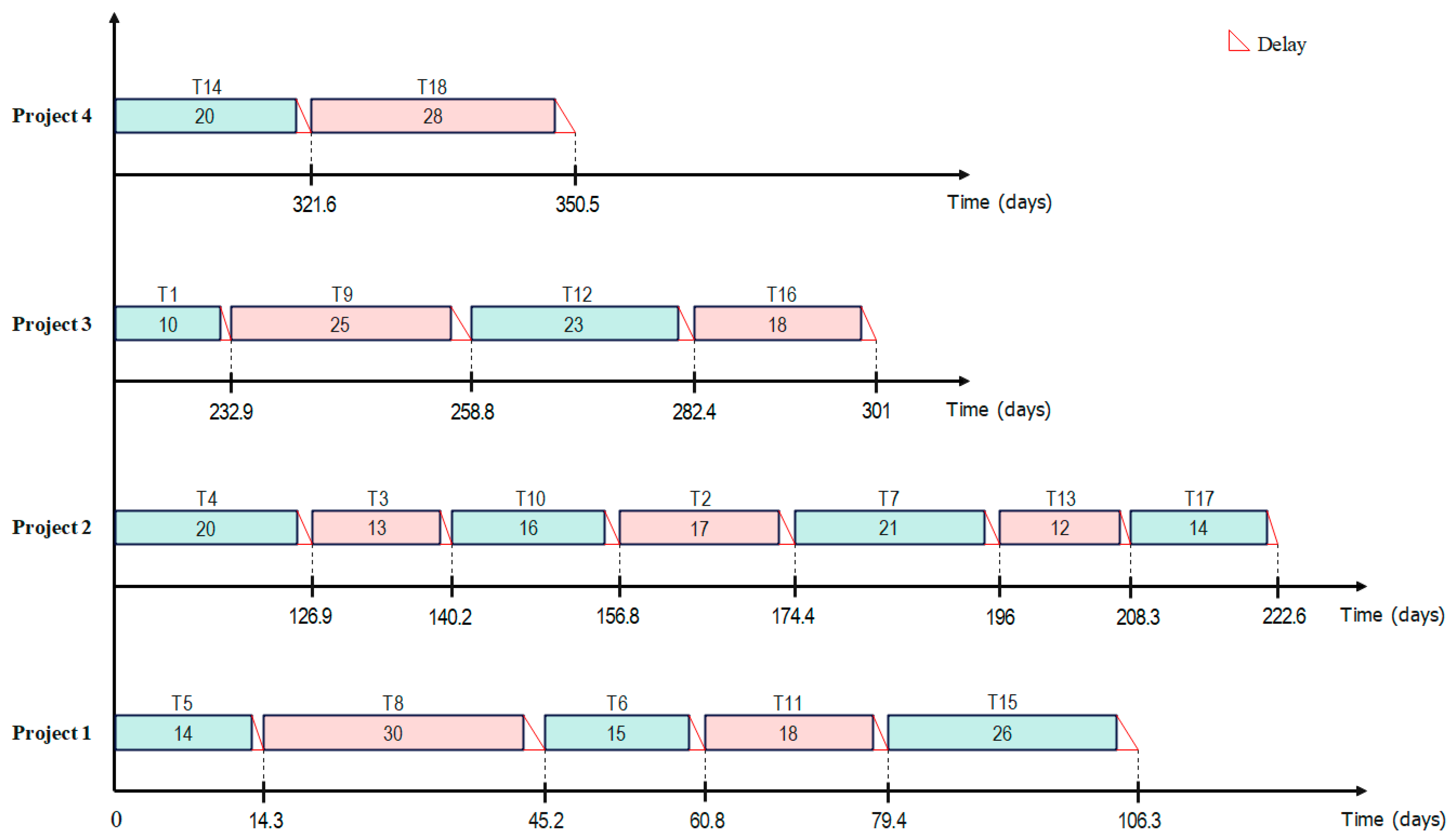
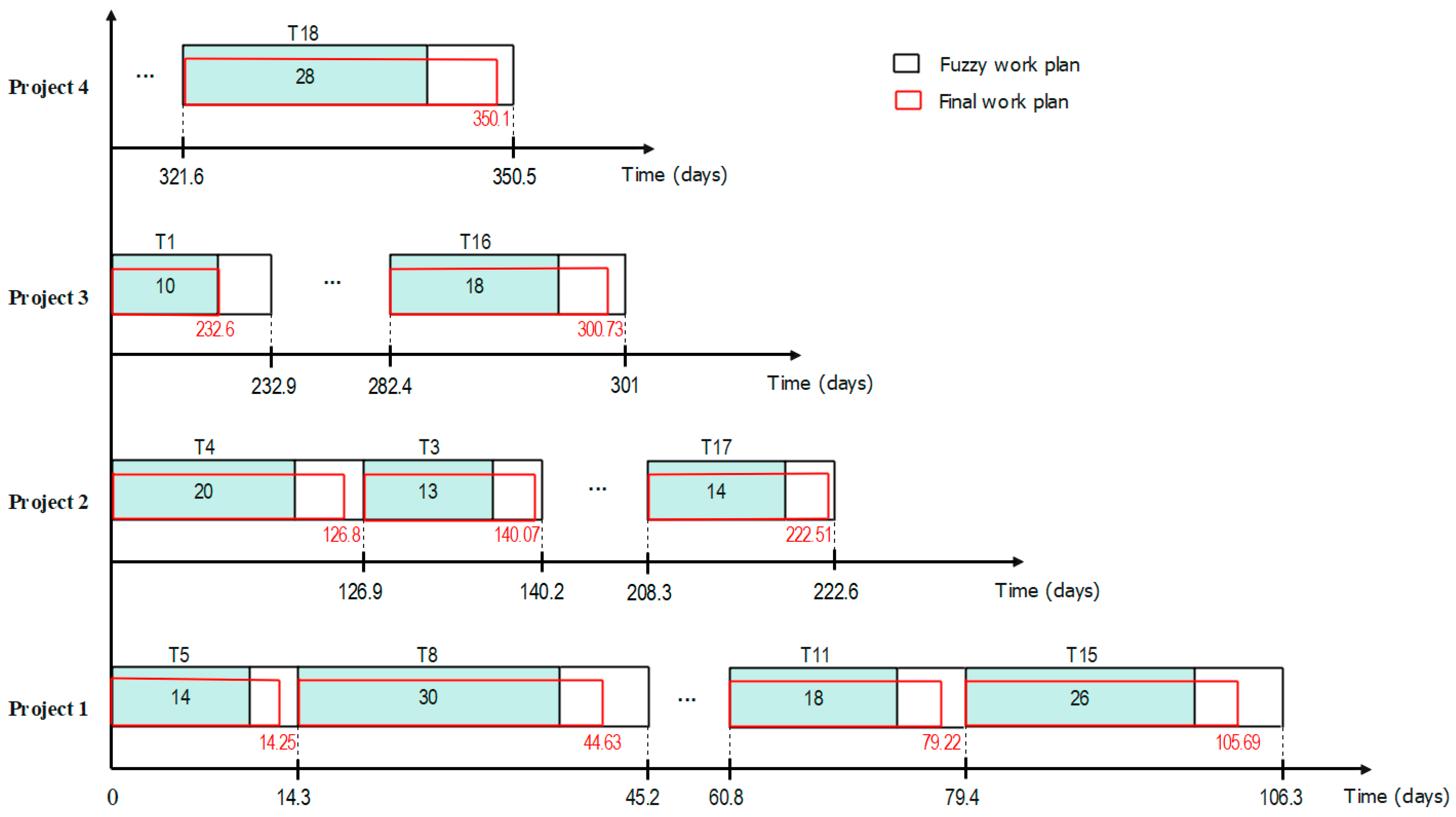
- With the parameters and decision variables, the fuzzy work plan for the machine is elaborated.
- Step 7:
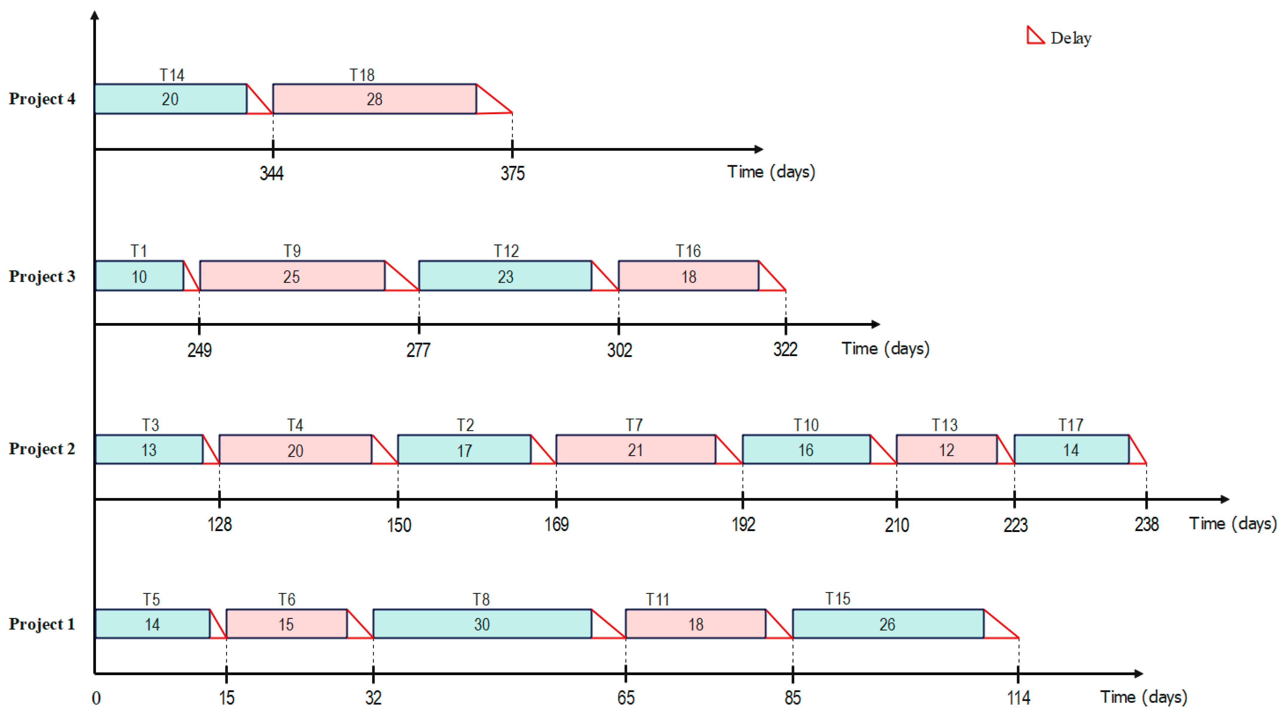
- With the incidents (delays) within the tolerances for each task, the final work plan for the machine must be elaborated.
3.4. Fuzzy Model Efficiency
4. Discussion
- (i)
- Extend the proposed model to deal with construction projects that contemplate imprecision with multiple machines.
- (ii)
- Use metaheuristics to solve the fuzzy optimization model when the number of tasks is large.
Author Contributions
Funding
Data Availability Statement
Conflicts of Interest
References
- Bettemir, H.; Birgönül, M.T. Network Analysis Algorithm for the Solution of Discrete Time-Cost Trade-off Problem. KSCE J. Civ. Eng. 2017, 21, 1047–1058. [Google Scholar] [CrossRef]
- Eshtehardian, E.; Afshar, A.; Abbasnia, R. Fuzzy-Based MOGA Approach to Stochastic Time-Cost Trade-off Problem. Autom. Constr. 2009, 18, 692–701. [Google Scholar] [CrossRef]
- Alzara, M.; Kashiwagi, J.; Kashiwagi, D.; Al-Tassan, A. Using PIPS to Minimize Causes of Delay in Saudi Arabian Construction Projects: University Case Study. Procedia Eng. 2016, 145, 932–939. [Google Scholar] [CrossRef]
- Zheng, D.X.M.; Ng, S.T. Stochastic Time-Cost Optimization Model Incorporating Fuzzy Sets Theory and Nonreplaceable Front. J. Constr. Eng. Manag. 2005, 131, 176–186. [Google Scholar] [CrossRef]
- Senouci, A.B.; Mubarak, S.A. Multiobjective Optimization Model for Scheduling of Construction Projects under Extreme Weather. J. Civ. Eng. Manag. 2016, 22, 373–381. [Google Scholar] [CrossRef]
- Itoh, T.; Ishii, H. Fuzzy Due-Date Scheduling Problem with Fuzzy Processing Time. Int. Trans. Oper. Res. 1999, 6, 639–647. [Google Scholar] [CrossRef]
- Niu, Q.; Jiao, B.; Gu, X. Particle Swarm Optimization Combined with Genetic Operators for Job Shop Scheduling Problem with Fuzzy Processing Time. Appl. Math. Comput. 2008, 205, 148–158. [Google Scholar] [CrossRef]
- Knyazeva, M.; Bozhenyuk, A.; Rozenberg, I. Resource-Constrained Project Scheduling Approach Under Fuzzy Conditions. Procedia Comput. Sci. 2015, 77, 56–64. [Google Scholar] [CrossRef]
- Al-Zarrad, M.A.; Fonseca, D. A New Model to Improve Project Time-Cost Trade-off in Uncertain Environments. In Contem-Porary Issues and Research in Operations Management; University of Alabama: Tuscaloosa, AL, USA, 2018; Volume 6, pp. 96–112. [Google Scholar]
- Nguyen, D.-T.; Le-Hoai, L.; Tarigan, P.B.; Tran, D.-H. Tradeoff Time Cost Quality in Repetitive Construction Project Using Fuzzy Logic Approach and Symbiotic Organism Search Algorithm. Alex. Eng. J. 2021, 61, 1499–1518. [Google Scholar] [CrossRef]
- Fernandez, N.A.; Segura, F.G.; Pino, M.E.M.; Chavil, W.J.Q.; Ruiz, A.D.; Sánchez, J.L.C. Optimization Model that Minimizes the Penalty Caused by Delayed Delivery of Construction Projects. Int. J. Prof. Bus. Rev. 2023, 8, e02553. [Google Scholar] [CrossRef]
- Lai, Y.-J.; Hwang, C.-L. Fuzzy Mathematical Programming; Springer: Berlín/Heidelberg, Germany, 1992; Volume 394. [Google Scholar]
- Gutiérrez, F.A. Un Modelo de Optimización Difusa para el Problema de Atraque de Barcos. Ph.D. Thesis, Universidad Nacional de Trujillo, Trujillo, Peru, 2017. Available online: http://dspace.unitru.edu.pe/handle/UNITRU/8931 (accessed on 24 February 2024).
- Verdegay, J. Fuzzy Mathematical Programming. In Fuzzy Information and Decision Processes; University of Granada: Granada, Spain, 1982; pp. 231–237. [Google Scholar]


| Task | Processing Time Days | Tolerance Days |
|---|---|---|
| T1 | 10 | 1 |
| T2 | 17 | 2 |
| T3 | 13 | 1 |
| T4 | 20 | 2 |
| T5 | 14 | 1 |
| T6 | 15 | 2 |
| T7 | 21 | 2 |
| T8 | 30 | 3 |
| T9 | 25 | 3 |
| T10 | 16 | 2 |
| T11 | 18 | 2 |
| T12 | 23 | 2 |
| T13 | 12 | 1 |
| T14 | 20 | 2 |
| T15 | 26 | 3 |
| T16 | 18 | 2 |
| T17 | 14 | 1 |
| T18 | 28 | 3 |
| Projects | Delivery Time Days | Penalty Dollars/Day |
|---|---|---|
| 95 | 1000 | |
| 205 | 1600 | |
| 280 | 2500 | |
| 330 | 3000 |
| Non-Interference Restrictions | |
|---|---|
| Precedence Restrictions | ||
|---|---|---|
| Delivery Time Restrictions |
|---|
| Work Plan | Task Start () | Expected Processing Time () | Task Delay () | Final Processing Time () | Delivery Time () | Project Delay () | Penalty () |
|---|---|---|---|---|---|---|---|
| T5 | 0 | 14 | 0.3 | 14.3 | |||
| T8 | 14.3 | 30 | 0.9 | 30.9 | |||
| T6 | 45.2 | 15 | 0.6 | 15.6 | |||
| T11 | 60.8 | 18 | 0.6 | 18.6 | |||
| T15 | 79.4 | 26 | 0.9 | 26.9 | 95 | 11.3 | $1000 |
| T4 | 106.3 | 20 | 0.6 | 20.6 | |||
| T3 | 126.9 | 13 | 0.3 | 13.3 | |||
| T10 | 140.2 | 16 | 0.6 | 16.6 | |||
| T2 | 156.8 | 17 | 0.6 | 17.6 | |||
| T7 | 174.4 | 21 | 0.6 | 21.6 | |||
| T13 | 196 | 12 | 0.3 | 12.3 | |||
| T17 | 208.3 | 14 | 0.3 | 14.3 | 205 | 17.6 | $1600 |
| T1 | 222.6 | 10 | 0.3 | 10.3 | |||
| T9 | 232.9 | 25 | 0.9 | 25.9 | |||
| T12 | 258.8 | 23 | 0.6 | 23.6 | |||
| T16 | 282.4 | 18 | 0.6 | 18.6 | 280 | 21 | $2500 |
| T14 | 301 | 20 | 0.6 | 20.6 | |||
| T18 | 321.6 | 28 | 0.9 | 28.9 | 330 | 20.5 | $3000 |
| Optimum Penalty | $153,460 | ||||||
| (Dollars) | |
|---|---|
| 0 | 85,600 |
| 0.1 | 108,220 |
| 0.2 | 130,840 |
| 0.3 | 153,460 |
| 0.4 | 176,080 |
| 0.5 | 198,700 |
| 0.6 | 221,320 |
| 0.7 | 243,940 |
| 0.8 | 266,560 |
| 0.9 | 289,180 |
| 1 | 311,800 |
| Task | Delay Hours | Delay Days |
|---|---|---|
| T5 | 6 | 0.25 |
| T8 | 8 | 0.33 |
| T6 | 0 | 0.00 |
| T11 | 10 | 0.42 |
| T15 | 7 | 0.29 |
| T4 | 12 | 0.50 |
| T3 | 4 | 0.17 |
| T10 | 11 | 0.46 |
| T2 | 13 | 0.54 |
| T7 | 0 | 0.00 |
| T13 | 6 | 0.25 |
| T17 | 5 | 0.21 |
| T1 | 0 | 0.00 |
| T9 | 8 | 0.33 |
| T12 | 14 | 0.58 |
| T16 | 8 | 0.33 |
| T14 | 0 | 0.00 |
| T18 | 12 | 0.50 |
| Final Work Plan | Task Start () | Processing Time () | Delivery Time () | Project Delay () | Penalty () |
|---|---|---|---|---|---|
| T5 | 0 | 14.25 | |||
| T8 | 14.3 | 30.33 | |||
| T6 | 45.2 | 15.00 | |||
| T11 | 60.8 | 18.42 | |||
| T15 | 79.4 | 26.29 | 95 | 10.69 | $1000 |
| T4 | 106.3 | 20.50 | |||
| T3 | 126.9 | 13.17 | |||
| T10 | 140.2 | 16.46 | |||
| T2 | 156.8 | 17.54 | |||
| T7 | 174.4 | 21.00 | |||
| T13 | 196 | 12.25 | |||
| T17 | 208.3 | 14.21 | 205 | 17.51 | $1600 |
| T1 | 222.6 | 10.00 | |||
| T9 | 232.9 | 25.33 | |||
| T12 | 258.8 | 23.58 | |||
| T16 | 282.4 | 18.33 | 280 | 20.73 | $2500 |
| T14 | 301 | 20.00 | |||
| T18 | 321.6 | 28.50 | 330 | 20.1 | $3000 |
| Optimum Penalty | $150,831 | ||||
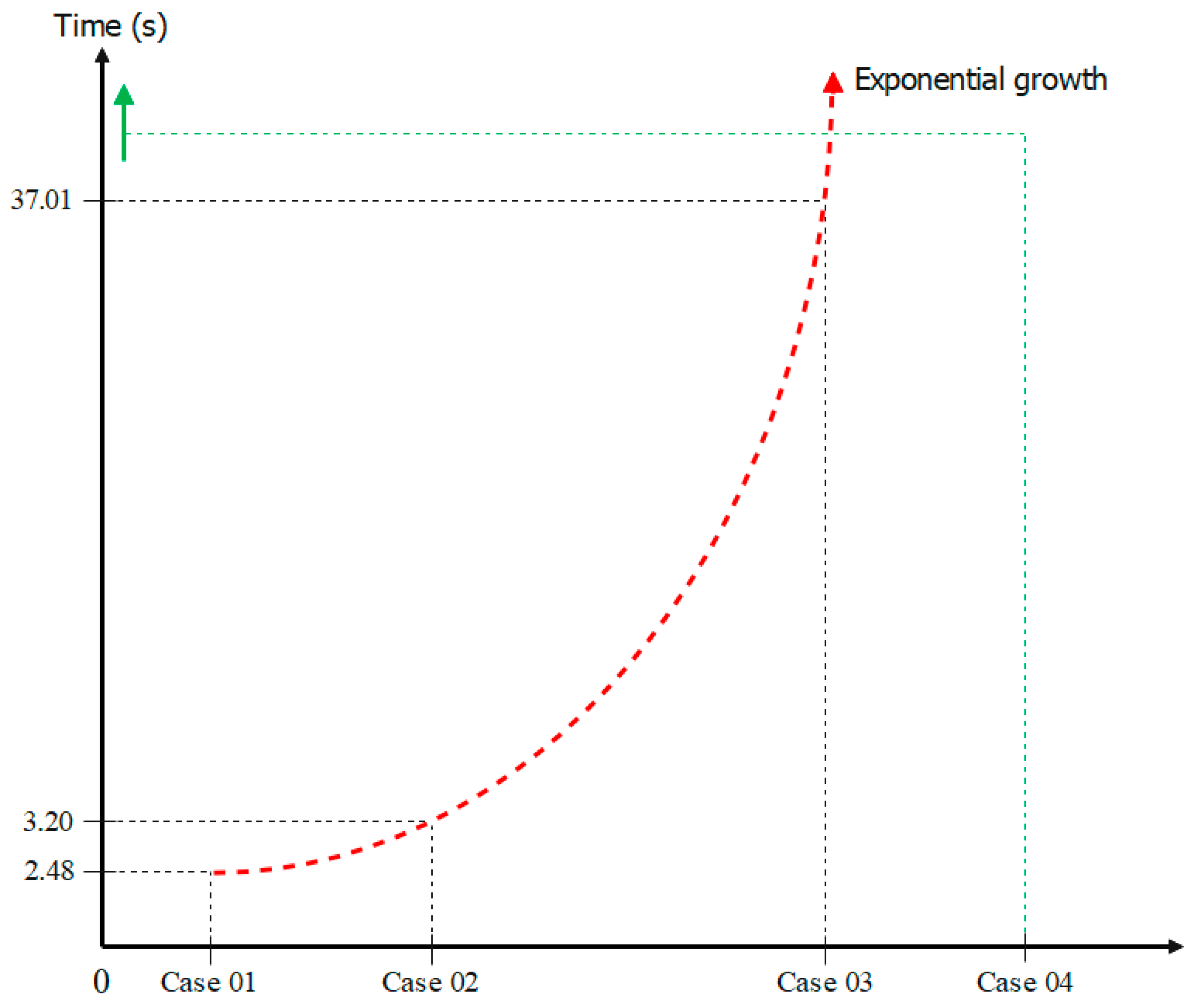
| Projects | Tasks | Computer Processing Time (s) | Optimum | Target Value (Dollars) | |
|---|---|---|---|---|---|
| Case 1 | 2 | 8 | 2.48 | yes | 204.30 |
| Case 2 | 3 | 15 | 3.20 | yes | 17,340.00 |
| Case 3 | 4 | 18 | 37.01 | yes | 153,460.00 |
| Case 4 | 4 | 27 | 29,700.00 | ------ | ------ |
Disclaimer/Publisher’s Note: The statements, opinions and data contained in all publications are solely those of the individual author(s) and contributor(s) and not of MDPI and/or the editor(s). MDPI and/or the editor(s) disclaim responsibility for any injury to people or property resulting from any ideas, methods, instructions or products referred to in the content. |
© 2024 by the authors. Licensee MDPI, Basel, Switzerland. This article is an open access article distributed under the terms and conditions of the Creative Commons Attribution (CC BY) license (https://creativecommons.org/licenses/by/4.0/).
Share and Cite
Arce Fernández, N.; Gutiérrez Segura, F.; Milla Pino, M.E.; Palomino Ojeda, J.M.; Ludeña Gutiérrez, A.L.; Chávez Santos, R. Fuzzy Optimization Model for Decision-Making in Single Machine Construction Project Planning. Mathematics 2024, 12, 1088. https://doi.org/10.3390/math12071088
Arce Fernández N, Gutiérrez Segura F, Milla Pino ME, Palomino Ojeda JM, Ludeña Gutiérrez AL, Chávez Santos R. Fuzzy Optimization Model for Decision-Making in Single Machine Construction Project Planning. Mathematics. 2024; 12(7):1088. https://doi.org/10.3390/math12071088
Chicago/Turabian StyleArce Fernández, Nilthon, Flabio Gutiérrez Segura, Manuel Emilio Milla Pino, Jose Manuel Palomino Ojeda, Alfredo Lázaro Ludeña Gutiérrez, and River Chávez Santos. 2024. "Fuzzy Optimization Model for Decision-Making in Single Machine Construction Project Planning" Mathematics 12, no. 7: 1088. https://doi.org/10.3390/math12071088
APA StyleArce Fernández, N., Gutiérrez Segura, F., Milla Pino, M. E., Palomino Ojeda, J. M., Ludeña Gutiérrez, A. L., & Chávez Santos, R. (2024). Fuzzy Optimization Model for Decision-Making in Single Machine Construction Project Planning. Mathematics, 12(7), 1088. https://doi.org/10.3390/math12071088