Approaches for Streamlining Performance Control by Monte Carlo Modeling

Abstract

For decades, cancer has remained a persistent health challenge; this project represents a significant stride towards refining treatment approaches and prognostic insights. Proton beam therapy, a radiation therapy modality employing high-energy protons to target various malignancies while minimizing damage to adjacent healthy tissue, holds immense promise. This study analyzes the relationship between delivered radiation doses and patient outcomes, using various approximation functions and graphical representations for comparison. Statistical analysis is performed through the Monte Carlo method based on repeated sampling to estimate the variables of interest in this analysis, namely, the survival rates, financial implications, and medical effectiveness of proton beam therapy. To this end, open-source data from research centers that publish patient outcomes were utilized. The second study considered the estimation of pay gaps that can have long-lasting effects, leading to differences in retirement savings, wealth accumulation, and overall financial security. After finding a representative sample containing the relevant variables that contribute to pay gaps, such as gender, race, experience, education, and job role, MC modeling is used to simulate a range of possible pay gap estimates. Based on the Monte Carlo results, a sensitivity analysis is performed to identify which variables have the most significant impact on pay gaps.

1. Introduction

Performance control incorporates management activities aimed at ensuring that a project’s performance closely aligns with a predefined set of desirable values. Performance is evaluated based on project performance indicators, including cost, schedule, labor productivity, materials consumption, and waste. The study of performance control has established the foundation for examining the requirements for control information from the perspective of management professionals at different levels of authority and responsibility within organizations. It additionally involves documenting the extent and level of detail of control information currently offered by existing monitoring systems and identifying similarities and differences in information monitoring and interpretation between these systems [1]. The connection between streamlining control and Monte Carlo methods lies in the use of simulation-based approaches to evaluate and prioritize risks in complex projects such as road pavement maintenance. Utilizing Monte Carlo simulations, a model can re-evaluate and prioritize risks, helping to efficiently manage and overcome the impacts of risks on construction projects. This method allows for a more comprehensive evaluation of risks from multiple perspectives and factors, aiding in informed decision-making to effectively control and mitigate potential risks [2].

The Monte Carlo method uses several random samples to approximate complex process outcomes or solve difficult mathematical problems. The Monte Carlo method was first established for atomic research during the Second World War, and it is now used in numerical simulations and probability analysis throughout many scientific and industrial fields. It is a powerful method for modeling and evaluating complicated systems in many domains, and has become an essential tool in numerical simulations and probability analysis, [3].

Modeling the effect of input variables on output quality is one of its uses. When paired with sensitivity analysis, which determines the inputs that have the biggest impact on a process, Monte Carlo simulations offer insightful information that can be used to guide decision-making and process improvements, see [4]. Bibliometrix is an R 4.3.2 software package designed for bibliometric analysis, enabling the quantitative evaluation of academic publications. It is implemented to examine citations evolution, authorship, and collaboration networks in scholarly writing. A Bibliometrix analysis shows that the keywords (performance control, mathematical modeling, and problem optimization) have been used together in the scientific world by 82 authors since 1998 and referred to by another 908 authors [5]. In 1998, Randall S. Sexton and Robert E. Dorsey demonstrated the superiority of genetic algorithms over backpropagation through a Monte Carlo analysis on seven test functions, showcasing its effectiveness in the in-sample, interpolation, and extrapolation scenarios [6]. According to Bibliometrix, this paper was the first significant mention of the statistical method’s commercial applicability in the scientific world.

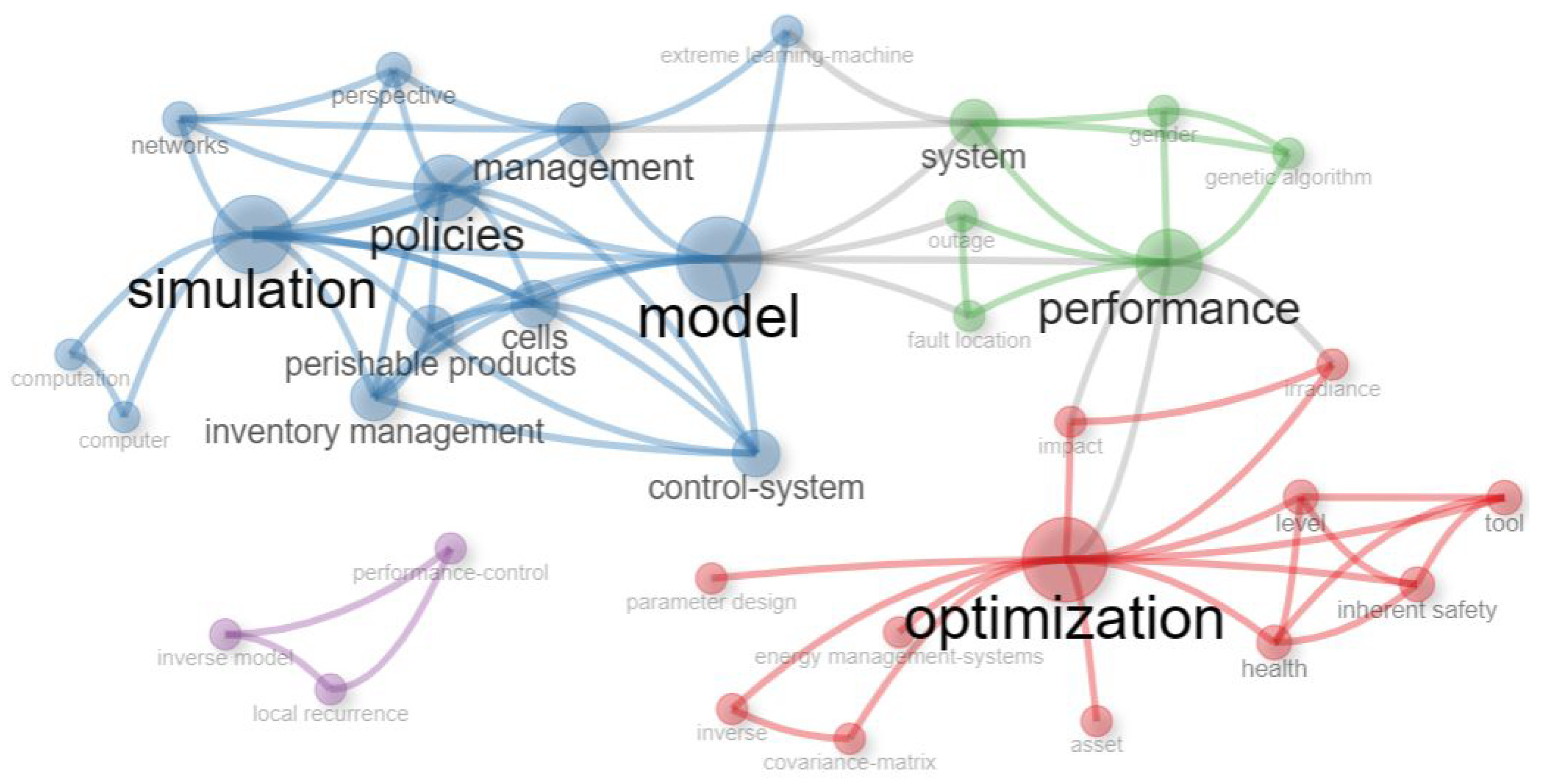
This has subsequently been proven in other studies, such as one from 2006 discussing improvements in product quality [7], and another [8] that inserts the Monte Carlo method into a sequential quadratic programming context. In the realm of performance control and mathematical modeling, optimization is key to enhancing system efficiency. Mathematical models serve as powerful tools helping to formulate effective policies and manage assets. Through simulation, these models offer a dynamic view of how different policies impact system performance. This integration facilitates strategic decision-making, enabling optimal asset management for resilient systems that adapt effectively to changing conditions. Its applicability in various domains is unquestionable, with performance optimization being among the most popular, as can be observed from Figure 1.

Bibliometrix is a robust tool for bibliometric analysis, facilitating seamless data importing and conversion to a data frame collection. Its versatile capabilities extend to data gathering through the Dimensions, PubMed, and Scopus APIs. This comprehensive platform further encompasses meticulous data filtering, ensuring precision in subsequent analyses. Bibliometrix empowers users with analytics and plots, spanning four crucial metrics: Sources, Authors, Documents, and Clustering by Coupling. The software delves into an in-depth examination of three knowledge structures—Conceptual, Intellectual, and Social Structure—providing a holistic understanding of scholarly landscapes through sophisticated bibliometric insights.

Figure 2 shows related idioms; their size is proportional to the frequency of mentions in scientific papers discussing this topic.

An interesting demonstration involving the fashion industry showed that statistical methods and machine learning algorithms can be used to improve business performance by enhancing sales forecasting. In 2019, Jonghyuk Kim and Hyunwoo Hwangbo demonstrated that stochastic control and optimization can improve issues related to product distribution, logistical costs, and inventory, improving the financial outcome of a company [9]. Use of the Monte Carlo method helped to facilitate project planning, resource allocation, and financial modeling. Numerous variables, such as advertising costs, retention rates, and sign-up rates, can be estimated for better risk management. Furthermore, as companies merge in order to expand, projections must be made, for which an estimation theory is needed [10].

Performance control and optimization via application of the Monte Carlo method have tremendous potential applicability in healthcare. For instance, medical image processing (CT, MRI) can be improved by examining Monte Carlo integration errors in graphics using Fourier analysis to enhance rendering algorithms, thereby ensuring that the algorithms are robust and reliable under different imaging conditions [11]. This is crucial for imaging systems, on which the diagnosis of numerous pathologies depend, as well as for new and better forms of cancer treatment such as proton radiotherapy [12]. Statistics have the potential to lowering high costs and expand accessibility, which are the most important problems around this revolutionary cancer therapy [13]. Through Monte Carlo simulations, the radiation dose for each patient can be optimized and treatment can be individualized, improving the technique even further [14].

This paper emphasizes the significance of Monte Carlo simulations in control and enhancement of performance in various domains, including finance, business, and medicine. Notably, the study emphasizes the potential of applying Monte Carlo methods as a way to analyze and improve multiple aspects of company operations, including managing cost and resolving salary discrepancies. Monte Carlo simulations can be used in many scenarios to enhance performance control by generating confidence intervals, such as radiotherapy in the medical context or compensation analysis in the business context.

This study explores pay gaps and cost efficiency modeling for proton beam therapy, highlighting impacts on social development and promoting equity, social justice, and economic sustainability. It establishes a framework for increased modeling and simulation techniques, enabling better policy development and resource allocation in a complex world. The study emphasizes exploring less explored areas of statistical analysis for societal growth and well-being. The Monte Carlo technique is used in both business and medical domains due to its versatility, motivating the study to push beyond customary limitations and explore new elements, potentially transforming business and medical landscapes.

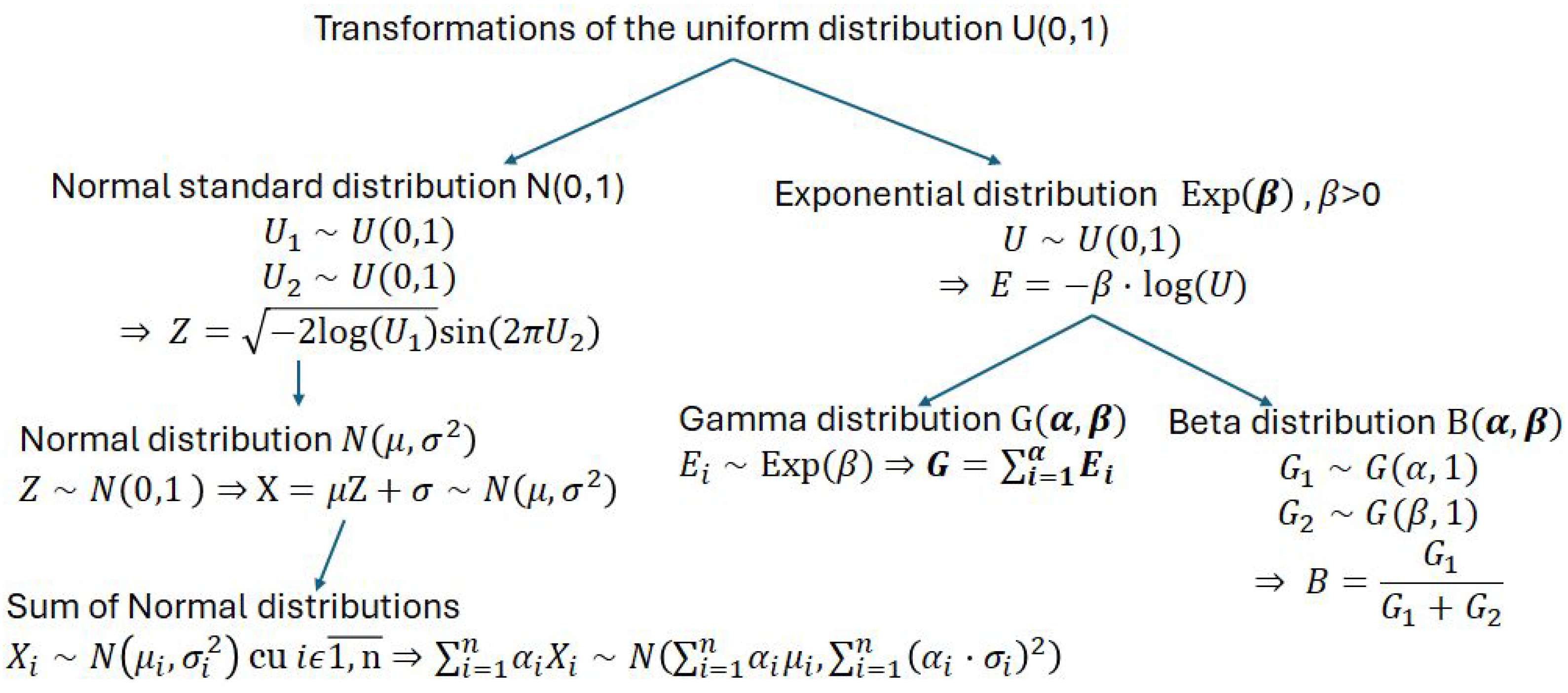
The rest of this paper is structured as follows. The next section addresses the statistical formalism for the Monte Carlo method, which encompasses probability theory, hypothesis testing, estimation, regression analysis, and experimental design. The subsequent section examines the outcomes of employing this technique in two domains: healthcare and economics. Section 2 of the paper presents significant statistical results, while Figure A1 illustrates the relationship among the $U(0,1)$, $N(\mu ,\sigma )$, Gamma$(\alpha ,\beta )$, and Beta$(\alpha ,\beta )$ distributions, which are useful for the Monte Carlo simulations presented in Section 3 and Section 4. Section 3 simulates the expenses of radiotherapy per fraction, considering the duration of radiotherapy in each fraction, which contributes to the overall cost. Section 4 addresses a pay gap model that uses Monte Carlo simulations to highlight the salary inequalities between men and women while considering variations in their education levels.

2. Methods and Algorithm

2.1. MC Applicability and Data Collection

The Monte Carlo method is a statistical method that represents a broad class of computational algorithms that rely on repeated random sampling to obtain numerical results [15]. The basic concept is to use randomness to solve problems that could be deterministic in principle but involve high costs or require lengthy computation. This method can also be useful for risk analysis when working with a large number of simulations by choosing the variable that has uncertainty and assigning it a random value [16].

MC modeling is an important mathematical tool used in many disciplines. It involves random sampling to study properties of systems with components that behave in random fashion, simulating the behavior of these systems by randomly generating variables describing the behavior of their components. MC modeling has numerous applications, including finance and risk analysis, physics and materials science, environmental science, healthcare and pharmaceuticals, energy and utilities, urban planning and transportation, and demographic studies.

This research includes Monte Carlo simulations based on high-cost experimental data related to the healthcare system through the relationship between the dose of radiation administered and the patient’s results in proton beam therapy. Deterministic analysis is based on various approximation functions and relatively empirical graphical representations.

The Monte Carlo method is used in the following section based on experimental data following repeated sampling (with numerical data taken from open access sources) to estimate the survival rates, financial implications, and medical effectiveness of proton beam therapy as the variables of interest in the analysis. Open-source data from research centers that publish patient outcomes are used.

2.2. Monte Carlo Modeling

Definition 1. 

Monte Carlo Method: Suppose that there is a numerical problem $\mathcal{P}$ to be solved with a solution λ. The Monte Carlo method for solving $\mathcal{P}$ consists of the following steps:

↫ 

a stochastic process X is appropriately associated such that it can be estimated λ

(e.g., $\lambda =E\left[\mathsf{\Lambda }\right(X\left)\right]$, $E\left[\mathsf{\Lambda }\right(X\left)\right]\to \lambda$ or $\mathsf{\Lambda }\left(X\right)$ converges in probability towards λ),

with Λ as a given function. $\mathsf{\Lambda }=\mathsf{\Lambda }\left(X\right)$ is an estimator of λ named the primary estimator.

↫ 

a selection $X_1,X_2,\dots ,X_n$ is simulated from X and an estimator ${\overline{\mathsf{\Lambda }}}_n$ of $\mathsf{\Lambda }\left(X\right)$ is computed.

In the case of $E\left[\mathsf{\Lambda }\right(X\left)\right]=\lambda$, the estimator for $\mathsf{\Lambda }\left(X\right)$ is ${\displaystyle {\overline{\mathsf{\Lambda }}}_n=\frac{1}{n}\sum _{i=1}^n\mathsf{\Lambda }\left(X_i\right),}$

called the secondary estimator.

↫ 

the solution of the problem $\left(P\right)$ is approximated with help of ${\overline{\mathsf{\Lambda }}}_n$.

Remark 1. 

If the primary estimator $\mathsf{\Lambda }\left(X\right)$ is unbiased, meaning $E\left[\mathsf{\Lambda }\right(X\left)\right]=\lambda$, then the secondary estimator ${\overline{\mathsf{\Lambda }}}_n$ typically follows the law of large numbers; therefore, ${\overline{\mathsf{\Lambda }}}_n\to \lambda$ in probability.

Remark 2. 

Using inverse method the that follows from Theorem A1, a simulation of a random variable $X\sim Exp\left(\lambda \right)$ with pdf $f\left(\mathrm{x}\right)=\lambda e^{-\lambda x}$, supp $f=(0,\infty )$ can be made.

The inverse of the distribution function $F\left(x\right)=1-e^{-\lambda x},x>0$ is provided for $u\in (0,1)$ by ${\displaystyle F^{-1}\left(u\right)=-\frac{1}{\lambda }log(1-u)}$; knowing $Y\sim U(0,1)\Rightarrow 1-Y\in U(0,1)$,

$$X=log\left(U^{-\frac{1}{\lambda }}\right)\sim Exp\left(\lambda \right).$$

For the density function $F\left(x\right)=1-\alpha e^{-\alpha x^{\beta }},x>0$ with $\mathrm{U}\sim U(0,1)$,

$$X={\left[-\frac{1}{\alpha }log\left(\mathrm{U}\right)\right]}^{1/\beta }\sim Exp(\alpha ,\beta ).$$

Remark 3. 

As in Figure A1 is precised $X\sim G(\alpha ,\beta )$ could be simulated by the sum ${\displaystyle G=\sum _{i=1}^{\alpha }{E}_i}$ for $E_i\sim Exp\left(\beta \right)$, if α is a positive integer.

For the case when $\alpha$ is a real positive value but not an integer, the accept-=reject algorithm can be used (Theorem A3). The instrumental distribution $Y\sim G(\left[\alpha \right],\frac{1}{b})$ is used in the algorithm, with ${\displaystyle b=\frac{\left[\alpha \right]}{\alpha }<1}$ obtained looking for the maximum critical value of the ratio ${\displaystyle \frac{f\left(x\right)}{g\left(x\right)}=\left(\frac{x^{\alpha -1}{e}^{-x}}{\mathsf{\Gamma }\left(\alpha \right)}\right)/\left(\frac{x^{\left[\alpha \right]-1}{e}^{-x/b}}{b^{\left[\alpha \right]}\mathsf{\Gamma }\left(\alpha \right)}\right)=\frac{x^{\alpha -\left[\alpha \right]}}{b^{\left[\alpha \right]}}{e}^{-(1-1/b)x}}$ as a function of b.

Remark 4. 

The Monte Carlo integration method (MCIM) [17], as a numerical technique for approximating definite integrals using random sampling, uses random sampling to estimate the average value of a function over a given region and then multiplies this average by the volume (or area in 1D) of the region to obtain an approximation of the integral.

Using the Monte Carlo method, the integral ${\displaystyle {\int }_a^{b}f\left(x\right)dx}$ for a continuous function f over the closed and bounded interval $[a,b]$ can be computed. We can write the integral as

$${\displaystyle I\left(f\right)={\int }_a^{b}f\left(x\right)dx=(b-a){\int }_a^{b}f\left(x\right)\frac{1}{b-a}dx=(b-a)E\left[f\left(X\right)\right],}$$

(1)

where $X\sim U(a,b)$ is the distribution. The Monte Carlo technique is then used to generate a random sample $X_1,\dots ,X_n$ of size n from the $U(a,b)$ distribution and compute $Y_i=(b-a)f\left(X_i\right)$. Then, Y is an unbiased estimator of ${\displaystyle {\int }_a^{b}f\left(x\right)dx}$.

Example 1. 

Estimator for the integral $I\left(f\right)$ with MCIM

Let $X_1,X_2,\dots ,X_n\sim U(a,b)$ be i.i.d random variables generated and corresponding random sample numbers: $\left(x_1,\dots ,x_n\right)$ uniformly distributed between $\mathrm{a}$ and $\mathrm{b}$. We compute ${\displaystyle Q_n=\frac{b-a}{n}\sum _{i=1}^{n}f\left(x_i\right)}$, the first estimator for $I\left(f\right)$ such that ${\displaystyle \frac{Q_n-I\left(f\right)}{\sigma /\sqrt{n}}}$ convergence in distribution to $N(0,1)$. The estimator for the variance ${\displaystyle \widehat{\sigma }={\left({\displaystyle \sum _{i=1}^n\frac{{\left(f\left(x_i\right)-Q_n\right)}^2}{n-1}}\right)}^{1/2}}$ leads to the confidence interval for $I\left(f\right)$: $\left({\displaystyle Q_n-\frac{\widehat{\sigma }}{\sqrt{n}}{Z}_{\alpha /2},Q_n+\frac{\widehat{\sigma }}{\sqrt{n}}{Z}_{\alpha /2}}\right)$.

Example 2. 

Optimization of robustness output design process with MCM (see [8]).

The design parameter for a new product is important in relation to the robustness of its design, and its probability distribution largely determines the robustness of the production response in general. Process optimization is based on improving the estimation of these parameters through Monte Carlo simulation.

The MCM algorithm (see [18]) follows these steps:

Step 1:

Define the relationship between the design variables X and response output as a response surface model $f\left(x\right)=f\left(x_1,x_2,\cdots ,x_n\right)$.

Step 2:

Define the distribution characteristics of the design variables,

Step 3:

Consider the samples $x\left(j\right)={\left\{x_{j1},x_{j2},\cdots ,x_{jn}\right\}}^{\mathrm{T}}$ of the variables X.

Step 4:

Compute the error for the sample according to the output B,

$${\Delta }_{max}=g{\left\{x_{j1},x_{j2},\cdots ,x_{jn},B\right\}}^{\mathrm{T}}.$$

Step 5:

Verify if $Y_j={\Delta }_{imax}-\epsilon <0,\epsilon$ the maximum error considered.

Step 6:

Repeat Step 2–Step 5 k times and compute $K_T={\sum }_{j=1}^k{U}_j$, $U_j=\left\{\begin{array}{cc}0\hfill & Y_j>0\hfill \\ 1\hfill & Y_j<0\hfill \end{array}\right.$

Step 7:

Compute the reliability ratio $P=K_T/K$ and compare it with the accepted one (D).

If $P>D$, then stop; otherwise, proceed to Step 2 and modify the precision value of random design variables to enhance the reliability ratio and robustness of the manufacturing process. The manufacturing process is then optimized.

3. Streamlining Performance Control in Healthcare Systems

Cancer has been an occurring problem in various patients for decades, and this project might be a step towards an improved approach of treatment and pathological prognosis.

Proton beam therapy is a type of radiation therapy that uses protons to treat different types of malignancies. It functions by targeting the tumor with doses of high-energy protons, reducing the nearby healthy tissue. This can be an advantage for older and sicker patients; the precision of this type of therapy is especially beneficial for patients where the cancer is in an inoperable place, such as the spinal cord, brain, bones, and soft tissues.

Statistical analysis using the Monte Carlo method, a broad class of computational algorithms that rely on repeated sampling to obtain numerical results, is considered here to estimate the survival chances and the financial and medical efficiency of proton beam therapy. Data found in research centers that have published patient outcomes were used. A study was made of both financial and medical efficiency using statistical methods.

Due to its ability to evaluate stochastic processes, select input probability distributions via hypothesis testing, and specify correlations between simulated variants, Monte Carlo simulation was used as a streamlining option for cost efficiency through simulation of the survival rates and primary treatment cost. This method offers superior simulation accuracy and separates principal work items and unit price components effectively, leading to acceptable precision and error rates in cost estimation [19].

3.1. Dose Optimization in Proton Beam Therapy

The dependency between the administered radiation dose and the absorbed particles and energy, as well as the patient outcomes, were computed using different types of approximation functions and graphic representations. The mathematical relations (2) define the absorbed dose by the quantity of radiation energy and the equivalent dose by factoring in a biological coefficient (see [20]):

$$\begin{array}{cc}\hfill & D_{abs}=\frac{W}{m},\left[D_{abs}\right]=1Sv=\frac{1}{20}Gy,\hfill \\ \hfill & D_{eq}=\omega D_{abs},D_e=\lambda D_{eq},\hfill \\ \hfill & \left[De\right]=\left[D_{\mathrm{eq}}\right]=1\mathrm{J}/\mathrm{kg}=1Gy(\mathrm{Gray}).\hfill \end{array}$$

(2)

The absorbed dose is defined as the quotient of the average energy transferred by ionizing radiation to a substance and the mass of that substance. The equivalent dose is calculated by multiplying the absorbed dose, which is the average amount of radiation energy absorbed by a tissue or organ, by a specified factor ($\omega$) that accounts for the kind of radiation. The effective dose is calculated by multiplying a biological factor ($\lambda$) with the equivalent dose for each organ.

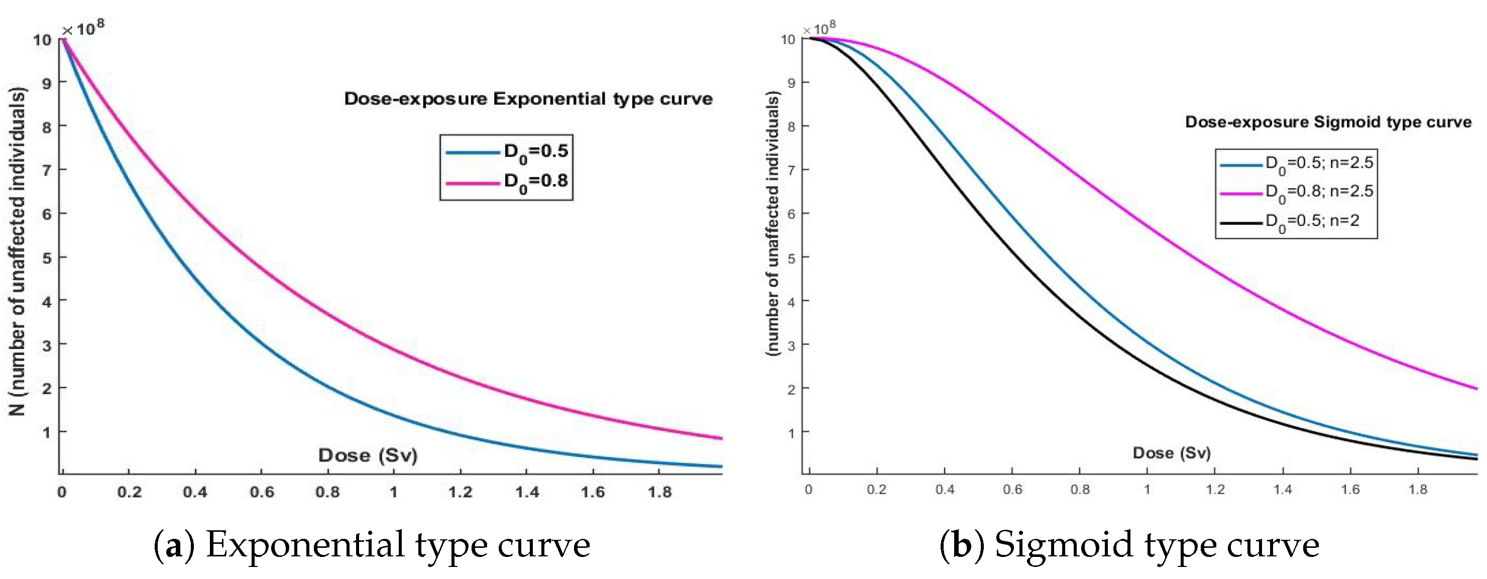
Graphical representations and approximation functions are employed to depict the dosage levels employed in the treatment of carcinomas. The exponential curve illustrates a decrease in the number of unaffected persons as the proton dose increases. Estimation of the unaffected individual influenced by the administrated dose and number of targets has the form ${\displaystyle \frac{N}{N_0}=e^{-kD}}$, graphically represented in Figure 3a.

On the other hand, the sigmoid graph incorporates the same analysis but is further influenced by n, the number of targets, which represents the number of cancer cells. This demonstrates that in the context of proton therapy it is possible to administer a greater dosage to effectively treat tumors, resulting in treatment of superior quality. Monitoring the prescribed dosage is essential, as it directly impacts the costs involved with this particular cancer treatment.

Figure 3b displays a sigmoid function created using an enhanced formula that incorporates both the administered dose and the quantity of targets in the body, specifically, the cancer cells affected by radiation ${\displaystyle \frac{N}{N_0}=1-{\left(1-e^{D/D_0}\right)}^n}$.

3.2. Cost Efficiency

Proton therapy, a promising treatment option in clinical and hospital settings [12], faces challenges due to its high cost compared to advanced photon therapy. Technological advancements are being made to reduce capital investment and operational costs. Instrumentation, facility layout, and treatment logistics are being improved to lower treatment costs. However, a significant reduction in treatment costs is not expected in the near future. The ultimate goal is to achieve a facility size and cost similar to photon treatment techniques; however, this will require further technological advancements and efficiency improvements. Despite these advancements, the high cost of proton therapy remains a significant obstacle to its widespread adoption.

Thorough cost estimates should take into account both direct factors and indirect factors such as impairment and decreased productivity [13]. Direct expenditures pertain specifically to medical treatments, whereas indirect expenses encompass labor costs, depreciation, maintenance, and overhead charges [21]. The main determinant of treatment costs in physical therapy is indirect charges, which can impede cost effectiveness. Treatment costs are influenced by factors such as capital investments, operating personnel charges, and maintenance needs. The method, fractions, and beams within each fraction have a considerable impact on cost estimation [13].

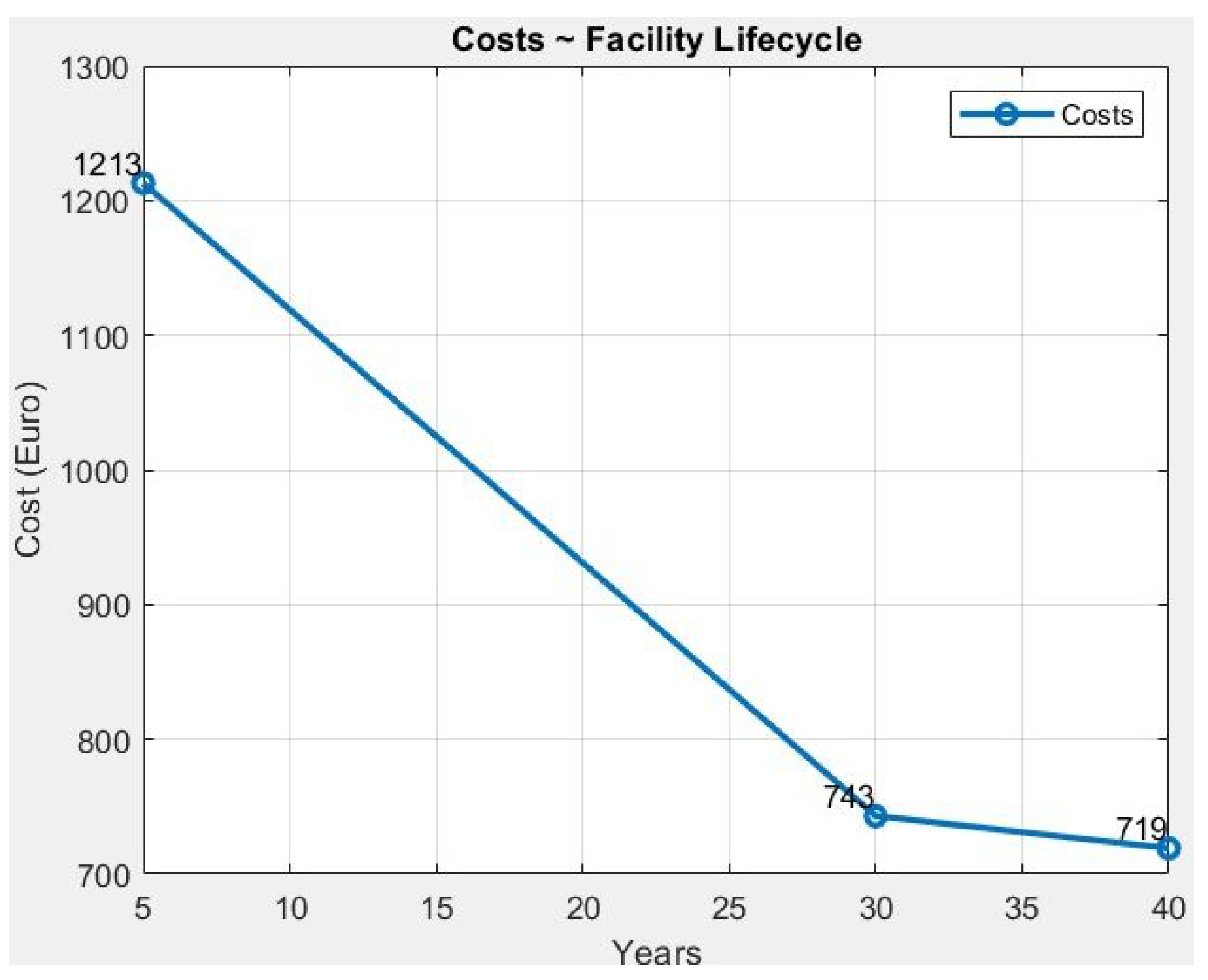
The therapeutic ratio of particle treatment is superior to that of photon therapy; nevertheless, the investment costs associated with particle therapy are relatively higher. The initial investment required for facilities that are solely proton-based, combination carbon ion/proton facilities, and photon facilities ranges from EUR 23.4 million to EUR 138.6 million. Proton therapy costs less per fraction than carbon-ion therapy but more than photon therapy. When compared to photon therapy, the cost ratio of particle therapy is considered to be 4.8 for establishments that provide both types of treatment, while the cost ratio for facilities that only provide proton therapy is recorded as 3.2 (see [22]). The cost per fraction of proton treatment ranges from EUR 743 to EUR 1300, resulting in an annual total cost of EUR 24.9 million for a center dedicated to proton therapy. The initial investment required for a proton-only establishment is around EUR 94.9 million (Figure 4).

The results of our research indicate that the costs incurred by each individual patient or every treatment course are expected to decrease dramatically when the number of patients undergoing therapy increases. As therapy advances, the duration of machine usage and the frequency of treatment sessions increase. The estimation of costs is significantly influenced by the procedure, the number of fractions, and the number of beams inside each fraction. There is a big issue regarding the lack of data regarding the consequences and expenses, and the collecting of appropriate data is the most important factor in determining reimbursement. The difficulties that are connected with estimating the costs of proton therapy include the limited availability of literature data, limitations in terms of methodology, and the possibility of differences between reimbursement estimates and actual treatment charges [23]. The significance of Monte Carlo simulations in this study is to analyse and improve the costs associated with proton beam therapy. In order to maximize this treatment’s potential, further mathematical analysis and modeling can be performed using Monte Carlo simulations to improve costs [24].

The results of these simulations provide valuable information that may be used to assess the efficacy and safety of various potential treatment strategies.

Using data from [13] (Table 1), the estimator $\widehat{E}=0.925$ for the mean $E\left[X\right]$ and standard error estimator $\widehat{V}=0.02$ for the $D\left[X\right]$, shape parameter ${\displaystyle k=\alpha =\frac{E{\left[X\right]}^2}{D\left[X\right]}}$, and scale parameter ${\displaystyle \theta =\frac{D\left[X\right]}{E\left[X\right]}=\frac{1}{\beta }}$ were computed and the Gamma($\alpha ,\beta$) 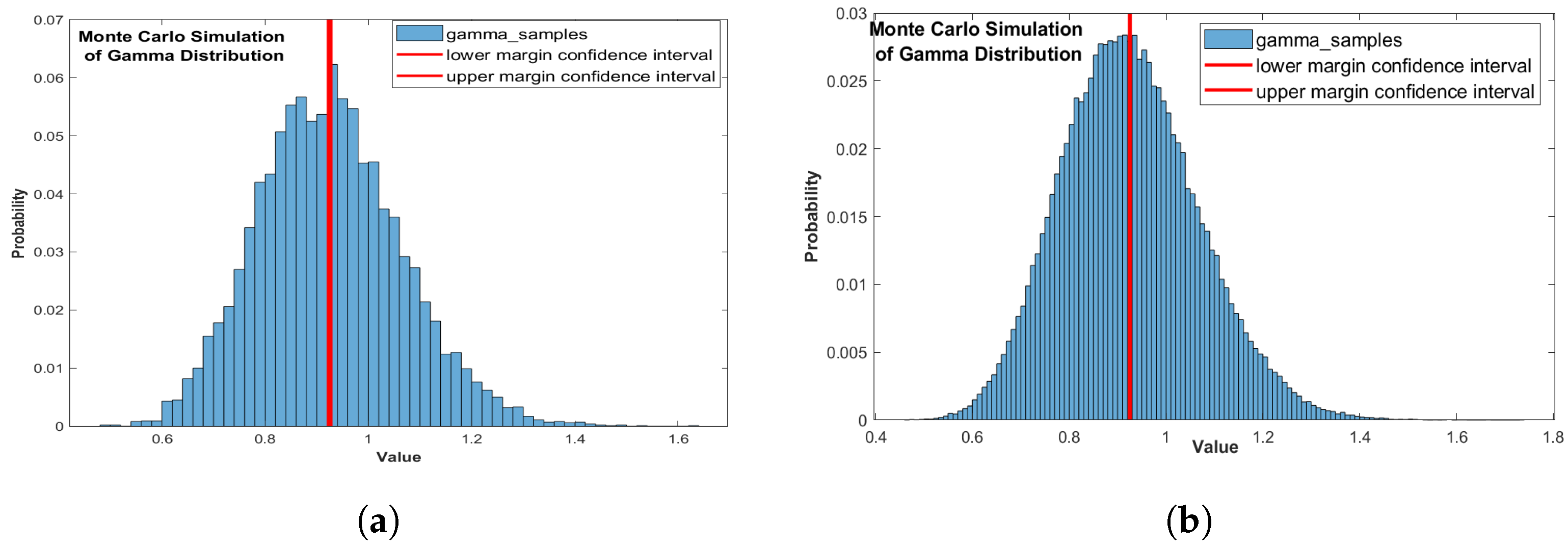distribution for the Survival rates (per three-month cycle) was plotted via Monte Carlo simulations for different numbers of samples, as shown in Figure 5.

In Figure 5a, for $n=\mathrm{10,000}$ number of samples we obtain a confidence interval of $[0.92222,0.92768]$; in Figure 5b, $n=\mathrm{100,000}$ is considered, and a confidence interval of $[0.92464,0.92639]$ is obtained for ($95\%$) significance.

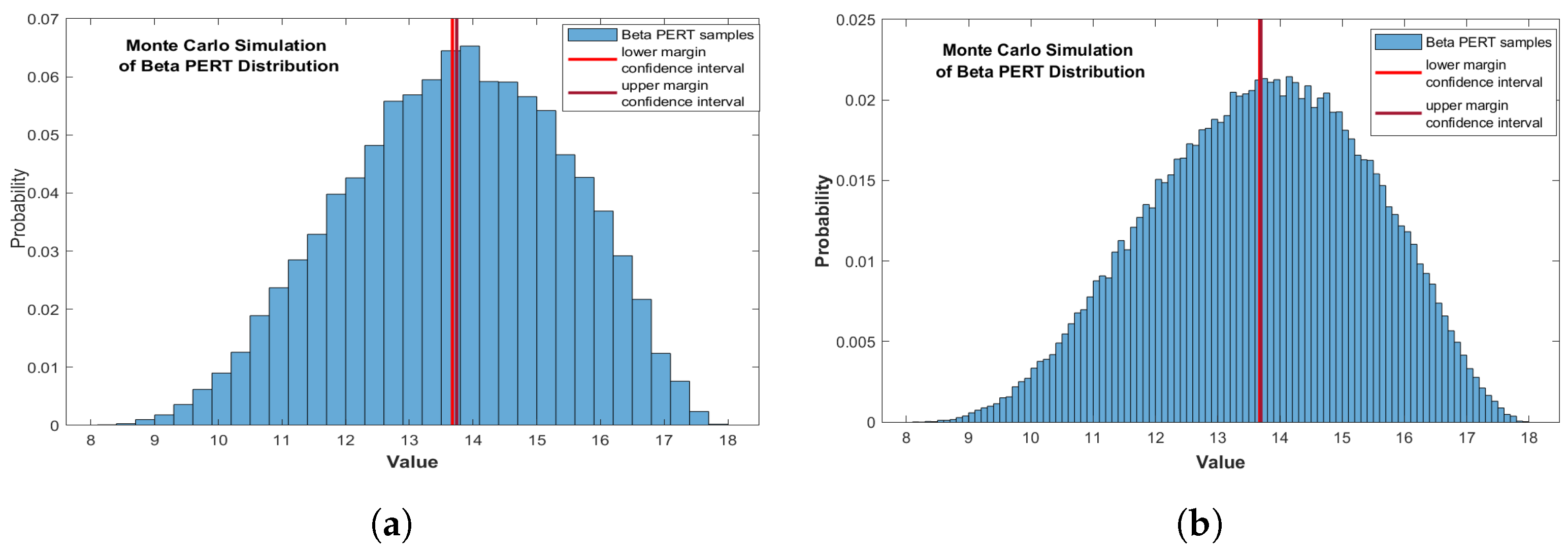
Using the minimum $a=8$, maximum value $c=18$ and the expected value ${\displaystyle \mu =\frac{a+4b+c}{6}=10}$ min (see [25] (Table 2) for the SE/range and the expected value), the most likely value $b=8.5$ is obtained. The Beta PERT $(a,b,c)$ distribution that models the primary treatment cost is MC simulated and depicted in Figure 6a for $n={10}^4$ number of samples, with a confidence interval $[13.6757,13.7437]$, and in Figure 6b for $n={10}^5$, with a confidence interval of $[13.674,13.6954]$ obtained for ($95\%$) significance.

A cost efficiency model for proton beam therapy can be written if we take into account primary treatment cost $c_{pt}$ (estimations presented in Figure 6), equipment cost,$c_{eq}$, and facility cost $c_f$ needed for a dose or for a multiple treatment ($c_{tc}=c_{pt}+c_{eq}+c_f$), taking account ABC principles in healthcare [26]. The facility cost $c_f$ is computed from the estimated cost per fraction depending on the lifecycle of a facility, shown in Figure 4, and the cost of a dose or multiple dose treatment according with the effective survival curve, which have the following form: $p=\left(1-p_m\right)e^{-\nu D_0}+p_m$ (see [27]). According to the TGP (Tumor Control Probability) model, $TCP=e^{-\gamma BED}$, $BED=nd\left({\displaystyle 1+\frac{d}{\alpha /\beta }}\right)$, $\alpha /\beta \in [0.5,5]Gy$ is the biologically effective dose (see [24,28,29]). The constant $p_m\in [0,1)$ is the survival rate at an infinite dose and $\nu >0$ is the slope parameter that determines how quickly the survival rate p transitions from 1 to $p_m$. Under the premise that $p_m$ is stable, the larger the $\nu$ is, the faster the p decreases; see [30].

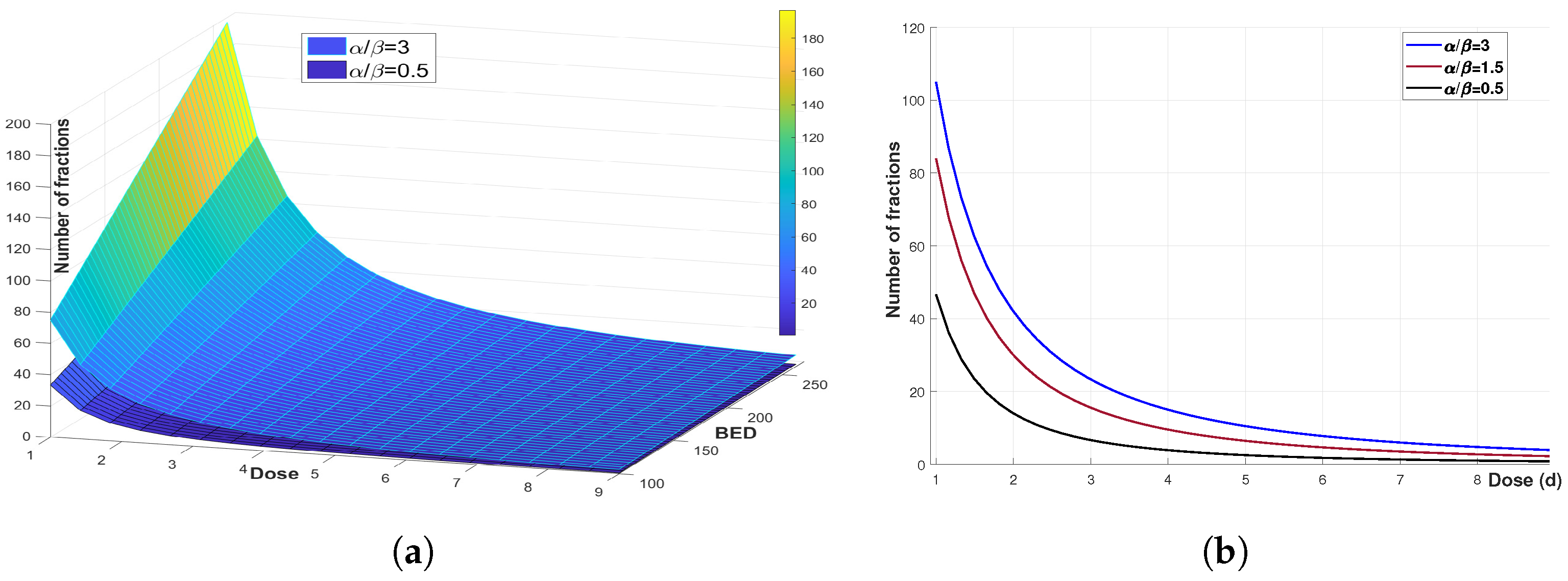
Figure 7a illustrates the correlation between the quantity of fractions, the dosage, and the BED (biologically effective dose) using the Linear-Quadratic (LQ) model formula. The Linear-Quadratic (LQ) model is utilized in radiation therapy to forecast the biological impacts of fractionation schemes. Furthermore, Figure 7b illustrates the correlation between dosage and the quantity of fractions. It is evident that the dosage and BED rise as the number of fractions decreases. Based on the evidence, it can be inferred that a therapy with the lowest alpha–beta ratio, administering a dose of 2 Gy, would require 15 portions. The alpha–beta ratio is a useful tool for assessing radiation treatment plans, as it quantifies tissue vulnerability to radiation. Within the LQ model, the ratio can vary between 1 and 5 Gy. The variations in values can be attributed to disparities in tumor cell attributes, such as genetic mutations, cellular repair processes, and microenvironmental factors. These factors affect the response to radiation therapy and contribute to the observed diversity in sensitivity across and within patients.

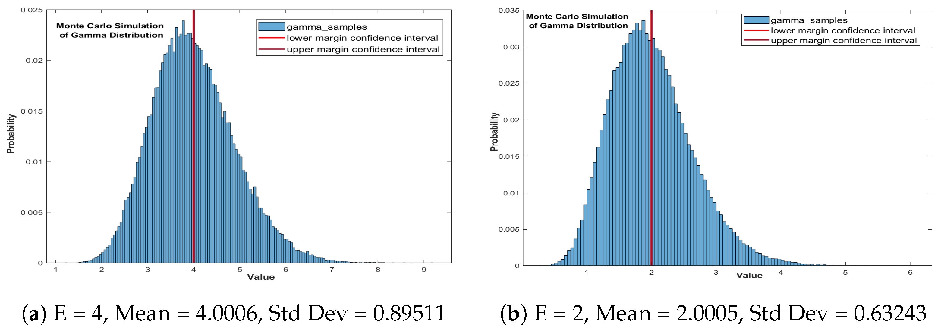
According to [24], the follow up cost per visit is EUR 97 and the number of follow-up visits for the first year and second year is a Gamma distribution with expected values of 4, and 2, respectively. Using MC simulations for the two cases, confidence intervals are obtained with probabilities depicted in Figure 8 and used to compute the secondary treatment costs, which include the costs of the probabilities of return in the first and second years.

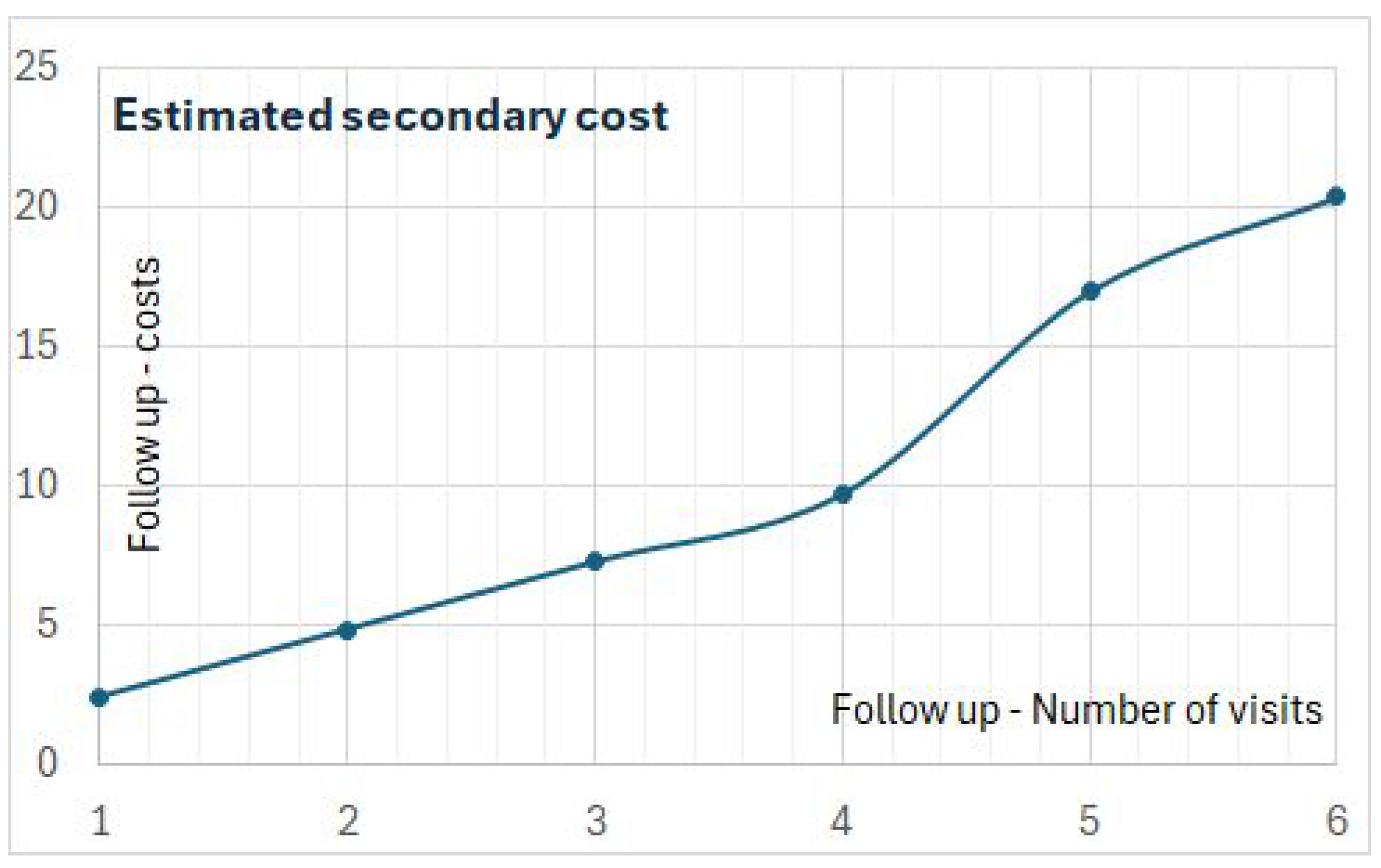
The total cost also includes these costs: $c_{tc}=c_t+c_{eq}+c_f$, with treatment cost expressed by primary cost and secondary cost ($c_t=c_{pt}+c_{st}$). In addition, the equipment cost is considered for the moment being fixed in EUR [14,030, 18,160] with an average of EUR 16,090, and the study could be continued for up to 5 years. For the follow-up of the next 3 years, MC simulations can be used with Gamma distribution with expected value $E=1$ each year and $V=0.2$ and with the value of EUR 97 per doctor visit to calculate the costs for each visit. For a more thorough checkup, an addional CT-scan cost is EUR 154 each year and can be simulated with the Gamma distribution function (Figure 9).

4. Business Model for Pay Gap Estimations

In Europe, the gender pay gap is an uncorrected statistic that provides a thorough picture of incomes and indicators that differentiate men and women in the workplace. A nuanced analysis detects that elements of the earnings inequality between genders can be attributed to two primary factors: first, differences in the average characteristics of male and female employees, and second, variations in the financial returns associated with these traits (see [31]). This intricate understanding emerges from the methodological study titled ‘Gender Pay Gaps in the European Union—a statistical analysis’, which meticulously investigates the drivers of the unadjusted gender pay gap, drawing insights from the 2018 edition of the Structure of Earnings Survey. Furthermore, the study of wage discrepancies in Europe goes into the differences between part-time and full-time work. Notably, while detailed data at this level is not available in all EU Member States, the discrepancies are significant. For part-time workers in 2021, the gender pay gap varied from −3.6% in Italy to 22.7% in Spain, with negative numbers reflecting women’s greater gross hourly wages, which are frequently impacted by selection biases (see [32]).

Addressing the wage gap in organizations involves a diverse approach that takes into account issues such as performance control and optimization. Establishing clear performance review methods that use objective criteria relevant to job functions is a good place to start, as it reduces the possibility of assessment bias. Regular pay equality audits which analyze data across demographics can help to discover and correct existing inequities. Implementing performance-based pay systems which tie salary to merit can help to align monetary rewards with individual contributions, thereby reducing the pay gap.

A statistical model that describes the relationship between compensation and the relevant variables can be considered through the Monte Carlo method. This could be a regression model or machine learning model that connects the input variables according to their distribution and uncertainty.

Analyzing the gender pay gap, different scenarios can be simulated by randomly assigning gender labels to individuals in the dataset while keeping other variables constant.

Let us consider a linear regression model between salary, months of experience, and education level:

$$\begin{array}{c}{S}_{ki}=S_{1i}+a_{1i}{M}_{ki}{\mathbf{1}}_{i[0,M_{ki}]}+a_{2i}E{d}_i+\epsilon ,i\in \left\{1,2\right\},k\in \overline{2,7},\hfill \\ S_{1i}=X_i\sim N({\mu }_i,{\sigma }_i^2),{\mu }_1-{\mu }_2=\Delta >0,\hfill \end{array}$$

(3)

where $S_{ki}$ is the salary of the individual gender ($i=1$ for men and $i=2$ for women) over the period of time k that depends on $M_{k·}=6(k-1)$ periods of experience (semestrial = six months), with the entire period under consideration being three years; here, $E{d}_i$ is a numerical representation of the individual’s education (1 for high school, 2 for bachelor’s, 3 for master’s, etc.).

For the MCM simulations, we assume that $\Delta =20\%{\mu }_1€$; moreover $a_{11}=a_{12}$, $a_{21}=a_{22}$ for the same k that are linearly increasing with a ${\delta }_1=10\%$ from the mean (that is, $100€$ and $80€$ if ${\mu }_1=1000€$ and ${\mu }_2=800€$) increasing arithmetic ratio in first two years and ${\delta }_2=8\%$ in the next two periods. In other cases, these parameters could be estimated from the employees’ company data.

To identify potential pay disparities, the predicted salary and difference $S_{k1}-S_{k2}$ could be studied for each semestrial period or at the end the three years.

Monte Carlo simulations to estimate pay gaps involve the following steps:

(a)

Specify the distribution of each variable and its probability distribution (e.g., years of experience, education level).

(b

Generate random samples by creating random samples from the specified distributions for each variable.

(c)

Calculate the salary for each sample.

(d)

Analyze pay gaps ⋄ and calculate pay gaps based on the characteristics of each simulated individual.

(e)

Run multiple Monte Carlo simulations to obtain a distribution of pay gap estimates ⋄ that reflects the uncertainty associated with the pay gap.

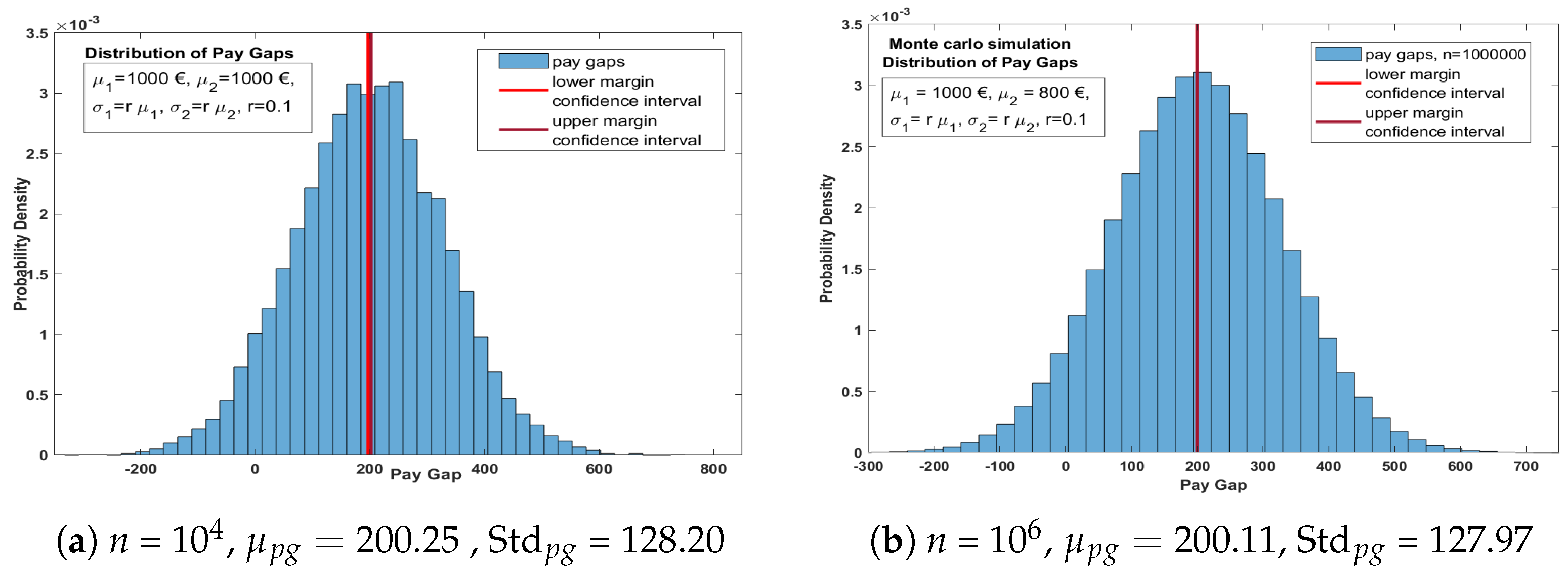
For $a_{22}=a_{21}$, according to Equation (3) and Figure A1, the salary at the end of the period k is $S_{ki}\sim N({\mu }_{ki},{\sigma }_{ki}^2)$ with

$$\begin{array}{c}\hfill \begin{array}{c}{\mu }_{ki}=M_{ki}{\mu }_i+(M_{ki}-1){\delta }_1,i\in \left\{1,2\right\},k\in \overline{2,7},\hfill \\ {\displaystyle {\sigma }_{ki}^2=\sum _{j=1}^{M_k}{\sigma }_i^2=M_k{\sigma }_i^2.}\hfill \end{array}\end{array}$$

(4)

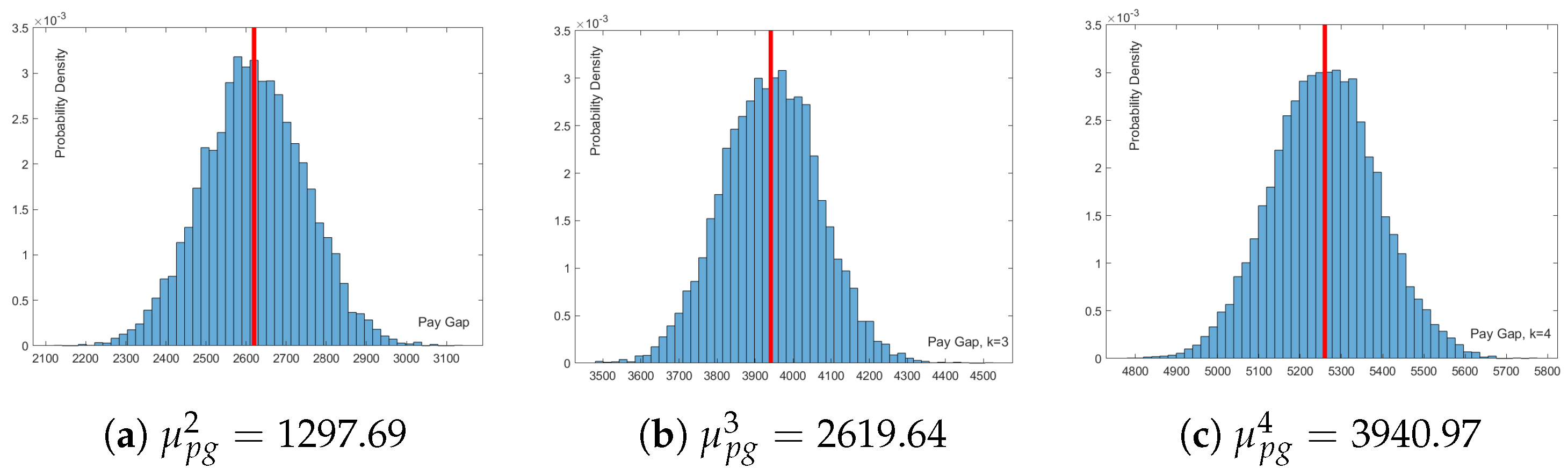
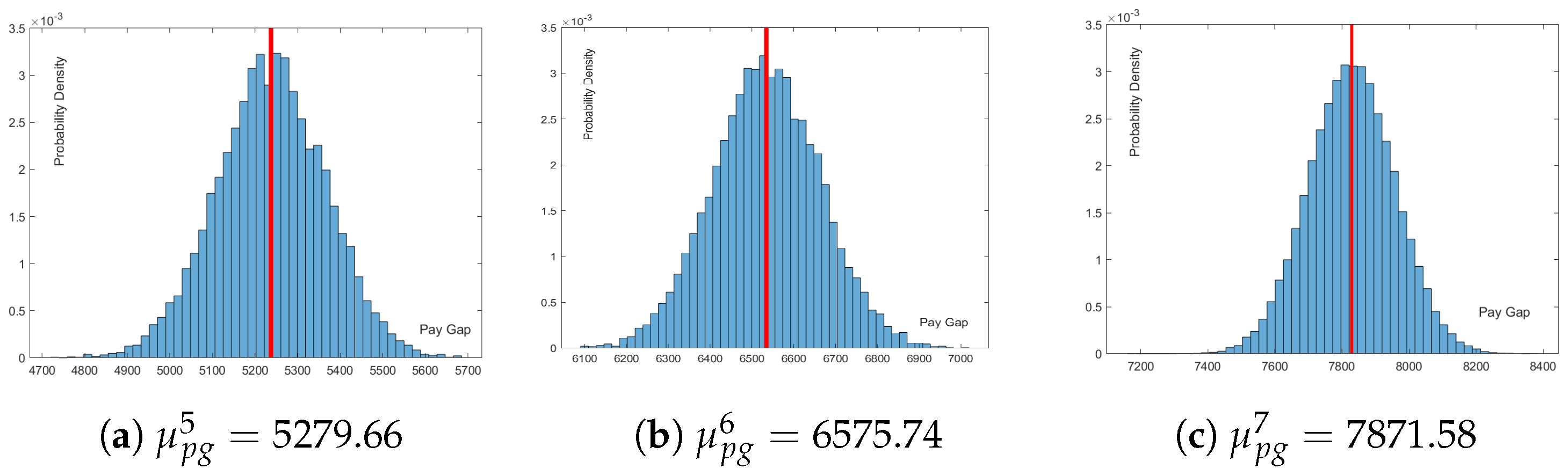
Denoting as ${\mu }_{pg}={\mu }_{11}-{\mu }_{12}$ the mean pay gap disparities after a first month, ${\mu }_{pg}^k={\mu }_{k1}-{\mu }_{k2}$ after period k, ${\mathrm{Std}}_{pg}$ the standard deviation after first month, and ${\mathrm{Std}}_{pg}^k$ the standard deviation after k period, Figure 10, Figure 11 and Figure 12 depict the MC simulations.

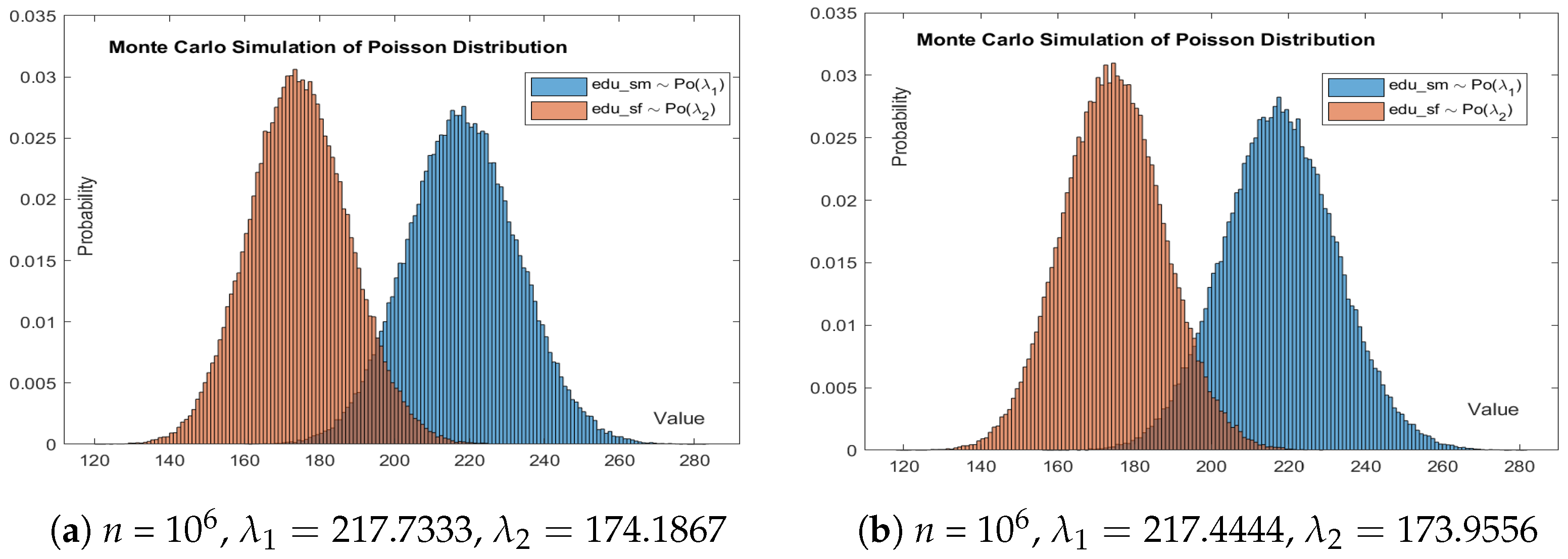
When graduating a new course, for example moving from a Bachelor’s degree to a Master’s, the mathematical model for the education that we could consider is the distribution for rare occurrences, namely, the Poisson distribution; in that sense, the end of the analyzed period is selected as the time frame for additional education, with a growth rate of 20%.

Figure 13 shows MC simulations of the additional income obtained from the education part for the two last periods; the two parameters ${\lambda }_1=217.7333$ and ${\lambda }_2=174.1867$ are computed from ${\mu }_{k1},{\mu }_{k2}$, with $k=6$ for Figure 13a and $k=7$ for Figure 13b.

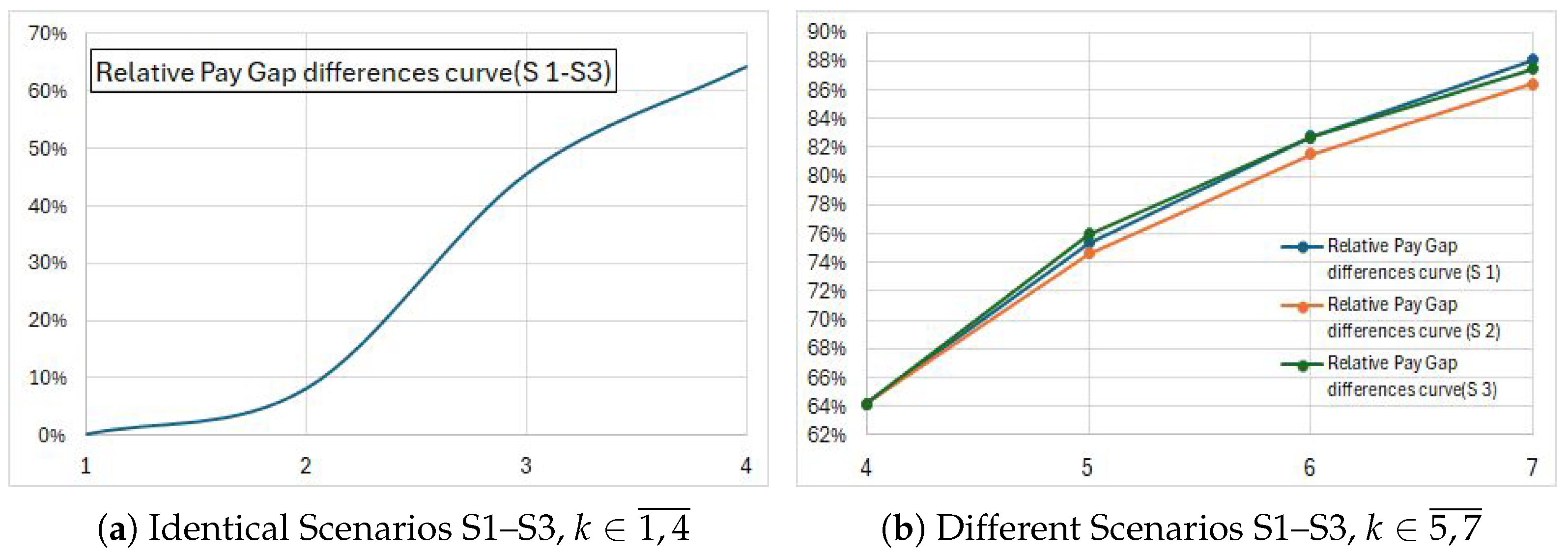
Figure 14 is dedicated to the accumulated income differences for the first four periods and for the last three. The three scenarios are identical for the first 2 years. Scenario ($S1$) maintains the same delta 1 increase until the end of the analyzed time period, scenario ($S2$) differs from ($S1$) by changing the percentage of increase ${\delta }_1$ in ${\delta }_2$, and scenario 3 additionally takes into account wage increases depending on education.

This concept demonstrates performance control by including the educational parameters of employees in their career advancement.

5. Conclusions

Monte Carlo simulations have emerged as an important tool for refining and improving proton beam therapy, a modern cancer treatment method. These techniques, which simulate the passage of proton beams through tissues with meticulous accuracy, provide for a full knowledge of dose and energy distribution, assisting in the formulation of more effective and focused treatment strategies. The costs related to radiotherapy in this research are essential to furthering the accessibility and evolution of healthcare in this direction.

In this study, it is underlined that the Monte Carlo method can be used to analyze and improve the way in which a business runs, whether in relation to costs or other issues such as salary differences. This research is important for modeling scenarios, revealing the possible impact of various solutions for closing the wage gap, benchmarking against industry norms, and requesting employee input to help create a more equal and inclusive corporate environment. Enhancing performance control is achieved by utilizing Monte Carlo simulations to establish a confidence interval in many situations, including radiotherapy and compensation analysis in a business setting. Values that deviate from the model are less congruent with the observed data, yet are crucial for error detection and enhancing efficiency.

The impact of statistical modeling is profound, as it provides insights into complex systems and facilitates predictions in a variety of fields, making it an essential tool for understanding and navigating our world’s complexities. These two selected scenarios for Monte Carlo simulations are significant in current society and are commonly debated among scientists. Both sections focus on reducing expenses and streamlining present management in discussions related to financial security and access to quality healthcare, which are essential human needs. Using Monte Carlo simulations helps enhance performance control in this manner by providing scenarios and risk analysis through estimation that aid decision-making in the systems.