A Multidimensional Principal Component Analysis via the C-Product Golub–Kahan–SVD for Classification and Face Recognition ^†

Abstract

Face recognition and identification are very important applications in machine learning. Due to the increasing amount of available data, traditional approaches based on matricization and matrix PCA methods can be difficult to implement. Moreover, the tensorial approaches are a natural choice, due to the mere structure of the databases, for example in the case of color images. Nevertheless, even though various authors proposed factorization strategies for tensors, the size of the considered tensors can pose some serious issues. Indeed, the most demanding part of the computational effort in recognition or identification problems resides in the training process. When only a few features are needed to construct the projection space, there is no need to compute a SVD on the whole data. Two versions of the tensor Golub–Kahan algorithm are considered in this manuscript, as an alternative to the classical use of the tensor SVD which is based on truncated strategies. In this paper, we consider the Tensor Tubal Golub–Kahan Principal Component Analysis method which purpose it to extract the main features of images using the tensor singular value decomposition (SVD) based on the tensor cosine product that uses the discrete cosine transform. This approach is applied for classification and face recognition and numerical tests show its effectiveness.

1. Introduction

An important challenge in the last few years was the extraction of the main information in large datasets, measurements, observations that appear in signal and hyperspectral image processing, data mining, machine learning. Due to the increasing volume of data required by these applications, approximative low-rank matrix and tensor factorizations play a fundamental role in extracting latent components. The idea is to replace the initial large and maybe noisy and ill conditioned large scale original data by a lower dimensional approximate representation obtained via a matrix or multi-way array factorization or decomposition. Principal Components Analysis is a widely used technique for image recognition or identification. In the matrix case, it involves the computation of eigenvalues or singular decompositions. In the tensor case, even though various factorization techniques have been developed over the last decades (high-order SVD (HOSVD), Candecomp–Parafac (CP) and Tucker decomposition), the recent tensor SVDs (t-SVD and c-SVD), based on the use of the tensor t-product or c-products offer a matrix-like framework for third-order tensors, see [1,2,3,4,5,6,7,8,9,10,11,12,13,14,15] for more details on recent work related to tensors and applications. In the present work, we consider third order tensors that could be defined as three dimensional arrays of data. As our study is based on the cosine transform product, we limit this work to three-order tensors.

For a given 3-mode tensor $\mathcal{X}\in {\mathbb{R}}^{n_1\times n_2\times n_3}$, we denote by $x_{i_1,i_2,i_3}$ the element $\left(i_1,i_2,i_3\right)$ of the tensor $\mathcal{X}$. A fiber is defined by fixing all the indexes except one. An element $c\in {\mathbb{R}}^{1\times 1\times n}$ is called a tubal-scalar or simply tube of length n. For more details refer to [1,2].

2. Definitions and Notations

2.1. Discrete Cosine Transformation

In this subsection we recall some definitions and properties of the discrete cosine transformation and the c-product of tensors. During recent years, many advances were made in order to establish a rigorous framework enabling the treatment of problems for which the data is stored in three-way tensors without having to resort to matricization [1,8]. One of the most important feature of such a framework is the definition of a tensor-tensor product as the t-product, based on the Fast Fourier Transform. For applications as image treatment, the tensor-tensor product based on the Discrete Cosine Transformation (DCT) has shown to be an interesting alternative to FFT. We now give some basic facts on the DCT and its associated tensor-tensor product. The DCT of a vector $v\in {\mathcal{R}}^n$ is defined by

$$\tilde{v}=C_{n}vs.\in {\mathcal{R}}^n,$$

(1)

where $C_n$ is the $n\times n$ discrete cosine transform matrix with entries

$${\left(C_n\right)}_{ij}=\sqrt{\frac{2-{\delta }_{i1}}{n}}cos\left({\displaystyle \frac{(i-1)(2j-1)\pi }{2n}}\right)1\le i,j\le n$$

with ${\delta }_{ij}$ is the Kronecker delta; see p. 150 in [16] for more details. It is known that the matrix $C_n$ is orthogonal, i.e., $C_n^T{C}_n=C_n{C}_n^T=I_n$; see [17]. Furthermore, for any vector $v\in {\mathbb{R}}^n$, the matrix vector multiplication $C_{n}v$ can be computed in $O\left(nlog\right(n\left)\right)$ operations. Moreover, Reference [17] have shown that a certain class of Toeplitz-plus-Hankel matrices can be diagonalized by $C_n$. More precisely, we have

$$C_n\mathtt{th}\left(v\right)C_n^{-1}=\mathrm{Diag}\left(\tilde{v}\right),$$

(2)

where

$$\mathtt{th}\left(v\right)=\underset{\mathrm{Toeplitz}}{\underbrace{\left(\begin{array}{cccc}{v}_1& v_2& \dots & v_n\\ v_2& v_1& \dots & v_3\\ ⋮& ⋮& \dots & ⋮\\ v_n& v_{n-1}& \dots & v_1\end{array}\right)}}+\underset{\mathrm{Hankel}}{\underbrace{\left(\begin{array}{cccc}{v}_2& \dots & v_n& 0\\ ⋮& ⋰& ⋰& v_n\\ v_n& 0& \dots & ⋮\\ 0& v_n& \dots & v_2\end{array}\right)}}$$

and $\mathrm{Diag}\left(\tilde{v}\right)$ is the diagonal matrix whose i-th diagonal element is ${\left(\tilde{v}\right)}_i$.

2.2. Definitions and Properties of the Cosine Product

In this subsection, we briefly review some concepts and notations, which play a central role for the elaboration of the tensor global iterative methods based on the c-product; see [18] for more details on the c-product.

Let $\mathcal{A}\in {\mathbb{R}}^{n_1\times n_2\times n_3}$ be a real valued third-order tensor, then the operations mat and its inverse ten are defined by

$$\begin{array}{cc}\hfill \mathtt{mat}\left(\mathcal{A}\right)=\underset{\mathrm{Block}\mathrm{Toeplitz}}{\underbrace{\left(\begin{array}{cccc}{A}_1& A_2& \dots & A_n\\ A_2& A_1& \dots & A_3\\ ⋮& ⋮& \dots & ⋮\\ A_n& A_{n-1}& \dots & A_1\end{array}\right)}}& +\underset{\mathrm{Block}\mathrm{Hankel}}{\underbrace{\left(\begin{array}{cccc}{A}_2& \dots & A_n& 0\\ ⋮& ⋰& ⋰& A_n\\ A_n& 0& \dots & ⋮\\ 0& A_n& \dots & A_2\end{array}\right)}}\in {\mathcal{R}}^{n_1{n}_3\times n_2{n}_3}\hfill \end{array}$$

and the inverse operation denoted by ten is simply defined by

$$\mathtt{ten}\left(\mathtt{mat}\right(\mathcal{A}\left)\right)=\mathcal{A}.$$

Let us denote $\tilde{\mathcal{A}}$ the tensor obtained by applying the DCT on all the tubes of the tensor $\mathcal{A}$. This operation and its inverse are implemented in the Matlab by the commands $\mathtt{dct}$ and $\mathtt{idct}$ as

$$\tilde{\mathcal{A}}=\mathtt{dct}(\mathcal{A},\left[\right],3),\mathrm{and}\mathtt{idct}(\tilde{\mathcal{A}},\left[\right],3)=\mathcal{A},$$

where $\mathtt{idct}$ denotes the Inverse Discrete Cosine Transform.

Remark 1.

Notice that the tensor$\tilde{\mathcal{A}}$can be computed by using the 3-mode product defined in [2] as follows:

$$\tilde{\mathcal{A}}=\mathcal{A}{\times }_{3}M$$

where M is the$n_3\times n_3$invertible matrix given by

$$M=W^{-1}{C}_{n_3}(I+Z)$$

where$C_{n_3}$denote de$n_3\times n_3$Discrete Cosine Transform DCT matrix,$W=\mathrm{diag}\left(C_{n_3}(:,1)\right)$is the diagonal matrix made of the first column of the DCT matrix, Z is$n_3\times n_3$circulant upshift matrix which can be computed in MATLAB using$W=\mathrm{diag}(\mathrm{ones}(n_3-1,1),1)$and I the$n_3\times n_3$identity matrix; see [18] for more details.

Let $\mathbf{A}$ be the matrix

$$\mathbf{A}=\left(\begin{array}{cccc}{A}^{\left(1\right)}& & & \\ & A^{\left(2\right)}& & \\ & & \ddots & \\ & & & A^{\left(n_3\right)}\end{array}\right)\in {\mathbb{R}}^{n_3{n}_1\times n_3{n}_2}$$

(3)

where the matrices $A^{\left(i\right)}$’s are the frontal slices of the tensor $\tilde{\mathcal{A}}$. The block matrix $\mathtt{mat}\left(\mathcal{A}\right)$ can also be block diagonalized by using the DCT matrix as follows

$$(C_{n_3}\otimes I_{n_1})\mathtt{mat}\left(\mathcal{A}\right)(C_{n_3}^T\otimes I_{n_2})=\mathbf{A}$$

(4)

Definition 1.

The c-product of two tensors$\mathcal{A}\in {\mathbb{R}}^{n_1\times n_2\times n_3}$and$\mathcal{B}\in {\mathbb{R}}^{n_2\times m\times n_3}$is the$n_1\times m\times n_3$tensor defined by:

$$\mathcal{A}{🟉}_c\mathcal{B}=\mathtt{ten}\left(\mathtt{mat}\left(\mathcal{A}\right)\mathtt{mat}\left(\mathcal{B}\right)\right).$$

Notice that from Equation (3), we can show that the product $\mathcal{C}=\mathcal{A}{🟉}_c\mathcal{B}$ is equivalent to $\mathbf{C}=\mathbf{A}\mathbf{B}$. Algorithm 1 allows us to compute, in an efficient way, the c-product of the tensors $\mathcal{A}$ and $\mathcal{B}$, see [18].

Algorithm 1 Computing the c-product.

Inputs: $\mathcal{A}\in {\mathbb{R}}^{n_1\times n_2\times n_3}$ and $\mathcal{B}\in {\mathbb{R}}^{n_2\times m\times n_3}$

Output: $\mathcal{C}=\mathcal{A}{🟉}_c\mathcal{B}\in {\mathbb{R}}^{n_1\times m\times n_3}$

1.  Compute $\tilde{\mathcal{A}}=\mathtt{dct}(\mathcal{A},\left[\right],3)$ and $\tilde{\mathcal{B}}=\mathtt{dct}(\mathcal{B},\left[\right],3)$.

2.  Compute each frontal slices of $\tilde{\mathcal{C}}$ by $$C^{\left(i\right)}=A^{\left(i\right)}{B}^{\left(i\right)}$$

3.  Compute $\mathcal{C}=\mathtt{idct}(\tilde{\mathcal{C}},\left[\right],3)$.

Next, give some definitions and remarks on the c-product and related topics.

Definition 2.

The identity tensor ${\mathcal{I}}_{n_1{n}_1{n}_3}$ is the tensor such that each frontal slice of ${\tilde{\mathcal{I}}}_{n_1{n}_1{n}_3}$ is the identity matrix $I_{n_1{n}_1}$.

An $n_1\times n_1\times n_3$ tensor $\mathcal{A}$ is said to be invertible if there exists a tensor $\mathcal{B}$ of order $n_1\times n_1\times n_3$ such that

$$\mathcal{A}{🟉}_c\mathcal{B}={\mathcal{I}}_{n_1{n}_1{n}_3}\mathrm{and}\mathcal{B}{🟉}_c\mathcal{A}={\mathcal{I}}_{n_1{n}_1{n}_3}.$$

In that case, we denote$\mathcal{B}={\mathcal{A}}^{-1}$. It is clear that$\mathcal{A}$is invertible if and only if$\mathtt{mat}\left(\mathcal{A}\right)$is invertible.

The inner scalar product is defined by

$${\displaystyle \langle \mathcal{A},\mathcal{B}\rangle =\sum _{i_1=1}^{n_1}\sum _{i_2=1}^{n_2}\sum _{i_3=1}^{n_3}{a}_{i_1{i}_2{i}_3}{b}_{i_1{i}_2{i}_3}}$$

and its corresponding norm is given by${\displaystyle {\parallel \mathcal{A}\parallel }_F=\sqrt{\langle \mathcal{A},\mathcal{A}\rangle }.}$

An $n_1\times n_1\times n_3$ tensor $\mathcal{Q}$ is said to be orthogonal if ${\mathcal{Q}}^T{🟉}_c\mathcal{Q}=\mathcal{Q}{🟉}_c{\mathcal{Q}}^T={\mathcal{I}}_{n_1{n}_1{n}_3}.$

Definition 3

([1]). A tensor is called f-diagonal if its frontal slices are diagonal matrices. It is called upper triangular if all its frontal slices are upper triangular.

Next we recall the Tensor Singular Value Decomposition of a tensor (Algorithm 2); more details can be found in [19].

Theorem 1.

Let $\mathcal{A}$ be an $n_1\times n_2\times n_3$ real-valued tensor. Then $\mathcal{A}$ can be factored as follows

$$\mathcal{A}=\mathcal{U}{🟉}_c\mathcal{S}{🟉}_c{\mathcal{V}}^T,$$

(5)

where $\mathcal{U}$ and $\mathcal{V}$ are orthogonal tensors of order $(n_1,n_1,n_3)$ and $(n_2,n_2,n_3)$, respectively, and $\mathcal{S}$ is an f-diagonal tensor of order $(n_1\times n_2\times n_3)$. This factorization is called Tensor Singular Value Decomposition (c-SVD) of the tensor $\mathcal{A}$.

Algorithm 2 The Tensor SVD (c-SVD).

Input:  $\mathcal{A}\in {\mathbb{R}}^{n_1\times n_2\times n_3}$Output: $\mathcal{U}$, $\mathcal{V}$ and $\mathcal{S}$.

1.  Compute $\tilde{\mathcal{A}}=\mathtt{dct}(\mathcal{A},\left[\right],3)$.

2.  Compute each frontal slices of $\tilde{\mathcal{U}}$, $\tilde{\mathcal{V}}$ and $\tilde{\mathcal{S}}$ from $\tilde{\mathcal{A}}$ as follows

(a)    for $i=1,\dots ,n_3$ $$[{\tilde{\mathcal{U}}}^{\left(i\right)},{\tilde{\mathcal{S}}}^{\left(i\right)},{\tilde{\mathcal{V}}}^{\left(i\right)}]=svd({\tilde{\mathcal{A}}}^{\left(i\right)})$$

(b)    End for

3.  Compute $\mathcal{U}=\mathtt{idct}(\tilde{\mathcal{U}},\left[\right],3)$, $\mathcal{S}=\mathtt{idct}(\tilde{\mathcal{S}},\left[\right],3)$ and $\mathcal{V}=\mathtt{idct}(\tilde{\mathcal{V}},\left[\right],3)$.

Remark 2.

As for the t-product [19], we can show that if $\mathcal{A}=\mathcal{U}{🟉}_c\mathcal{S}{🟉}_c{\mathcal{V}}^T$ is a c-SVD of the tensor $\mathcal{A}$, then we have

$${\displaystyle \sum _{k=1}^{n_3}{A}_k=\left({\displaystyle \sum _{k=1}^{n_3}{U}_k}\right)\left({\displaystyle \sum _{k=1}^{n_3}{S}_k}\right)\left({\displaystyle \sum _{k=1}^{n_3}{V}_k^T}\right),}$$

(6)

where $A_k$, $U_k$, $S_k$ and $V_k$ are the frontal slices of the tensors $\mathcal{A}$, $\mathcal{U}$, $\mathcal{S}$ and $\mathcal{V}$, respectively, and

$${\displaystyle \mathcal{A}=\sum _{i=1}^{min(n_1,n_2)}\mathcal{U}(:,i,:){🟉}_c\mathcal{S}(i,i,:){🟉}_c\mathcal{V}{(:,i,:)}^T.}$$

(7)

Theorem 2.

Let $\mathcal{A}=\mathcal{U}{🟉}_c\mathcal{S}{🟉}_c{\mathcal{V}}^T$ given by (5), and define for $k\le min(n_1,n_2)$ the tensor

$${\displaystyle {\mathcal{A}}_k=\sum _{i=1}^k\mathcal{U}(:,i,:){🟉}_c\mathcal{S}(i,i,:){🟉}_c\mathcal{V}{(:,i,:)}^T.}$$

(8)

Then

$${\mathcal{A}}_k=arg\underset{\mathcal{X}\in \mathcal{M}}{min}{\parallel {\mathcal{A}}_k-\mathcal{A}\parallel }_F,$$

(9)

where $\mathcal{M}=\{\mathcal{X}{🟉}_c\mathcal{Y};\mathcal{X}\in {\mathcal{R}}^{n_1\times k\times n_3},\mathcal{Y}\in {\mathcal{R}}^{k\times n_2\times n_3}\}$.

Note that when $n_3=1$ this theorem reduces to the well known Eckart–Young theorem for matrices [20].

Definition 4

(The tensor tubal-rank).Let $\mathcal{A}$ be an $n_1\times n_2\times n_3$ be a tensor and consider its c-SVD $\mathcal{A}=\mathcal{U}{🟉}_c\mathcal{S}{🟉}_c{\mathcal{V}}^T$. The tensor tubal rank of $\mathcal{A}$, denoted as rank${}_t$($\mathcal{A}$) is defined to be the number of non-zero tubes of the f-diagonal tensor $\mathcal{S}$, i.e.,

$${\mathrm{rank}}_t\left(\mathcal{A}\right)=\#\{i,\mathcal{S}(i,i,:)\ne 0\}.$$

Definition 5.

The multi-rank of the tensor $\mathcal{A}$ is a vector $p\in {\mathbb{R}}^{n_3}$ with the i-th element equal to the rank of the i-th frontal slice of $\tilde{\mathcal{A}}=\mathtt{fft}(\mathcal{A},\left[\right],3)$, i.e.,

$$p\left(i\right)=rank(A^{\left(i\right)}),i=1,\dots ,n_3.$$

The well known QR matrix decomposition can also be extended to the tensor case; see [19].

Theorem 3.

Let $\mathcal{A}$ be a real-valued tensor of order $n_1\times n_2\times n_3$. Then $\mathcal{A}$ can be factored as follows

$$\mathcal{A}=\mathcal{Q}{🟉}_c\mathcal{R},$$

(10)

where $\mathcal{Q}$ is an $n_1\times n_1\times n_3$ orthogonal tensor and $\mathcal{R}$ is an $n_1\times n_1\times n_3$ f-upper triangular tensor.

3. Tensor Principal Component Analysis for Face Recognition

Principle Component Analysis (PCA) is a widely used technique in image classification and face recognition. Many approaches involve a conversion of color images to grayscale in order to reduce the training cost. Nevertheless, for some applications, color an is important feature and tensor based approaches offer the possibility to take it into account. Moreover, especially in the case of facial recognition, it allows the treatment of enriched databases including for instance additional biometric information. However, one has to bear in mind that the computational cost is an important issue as the volume of data can be very large. We first recall some background facts on the matrix based approach.

3.1. The Matrix Case

One of the simplest and most effective PCA approaches used in face recognition systems is the so-called eigenface approach. This approach transforms faces into a small set of essential characteristics, eigenfaces, which are the main components of the initial set of learning images (training set). Recognition is done by projecting a test image in the eigenface subspace, after which the person is classified by comparing its position in eigenface space with the position of known individuals. The advantage of this approach over other face recognition strategies resides in its simplicity, speed and insensitivity to small or gradual changes on the face.

The process is defined as follows: Consider a set of training faces $I_1$, $I_2$, …, $I_p$. All the face images have the same size: $n\times m$. Each face $I_i$ is transformed into a vector $x_i$ using the operation $vec$: $x_i=vec\left(I_i\right)$. These vectors are columns of the $nm\times p$ matrix

$$X=[x_1,\dots ,x_p].$$

We compute the average image ${\displaystyle \mu =\frac{1}{p}\sum _{i=1}^p{x}_i.}$ Set ${\overline{x}}_i=x_i-\mu$ and consider the new matrices

$$\overline{X}=[{\overline{x}}_1,\dots ,{\overline{x}}_p],\mathrm{and}C=\overline{X}{\overline{X}}^T.$$

Notice that the $nm\times nm$ covariance matrix $C=\overline{X}{\overline{X}}^T$ can be very large. Therefore, the computation of the $nm$ eigenvalues and the corresponding eigenvectors (eigenfaces) can be very difficult. To circumvent this issue, we instead consider the smaller $p\times p$ matrix $L={\overline{X}}^T\overline{X}$.

Let $v_i$ be an eigenvector of L then $L{v}_i={\overline{X}}^T\overline{X}{v}_i={\lambda }_i{v}_i$ and

$$\overline{X}L{v}_i=\overline{X}{\overline{X}}^T\overline{X}{v}_i={\lambda }_i\overline{X}{v}_i,$$

which shows that $\overline{X}{v}_i$ is an eigenvector of the covariance matrix $C=\overline{X}{\overline{X}}^T$.

The p eigenvectors of $L={\overline{X}}^T\overline{X}$ are then used to find the p eigenvectors $u_i=\overline{X}{v}_i$ of C that form the eigenface space. We keep only k eigenvectors corresponding to the largest k eigenvalues (eigenfaces corresponding to small eigenvalues can be omitted, as they explain only a small part of characteristic features of the faces.)

The next step consists of projecting each image of the training sample onto the eigenface space spanned by the orthogonal vectors $u_1,\dots ,u_k$:

$${\mathcal{U}}_k=span\{u_1,\dots ,u_k\},\mathrm{with}{U}_k=[u_1,\dots ,u_k]$$

The matrix $U_k{U}_k^T$ is an orthogonal projector onto the subspace ${\mathcal{U}}_k$. A face image can be projected onto this face space as $y_i=U_k^T(x_i-\mu ).$

We now give the steps of an image classification process based on this approach:

Let $x=vec\left(I\right)$ be a test vector-image and project it onto the face space to get $y=U_k^T(x-\mu ).$ Notice that the reconstructed image is given by

$$x^r={\tilde{U}}_{k}y+\mu .$$

Compute the Euclidean distance

$${ϵ}_i=\parallel y-y_i\parallel ,i=1,\dots ,k.$$

A face is classified as belonging to the class l when the minimum l is below some chosen threshold $\theta$ Set

$${\displaystyle \theta =\frac{1}{2}\underset{i,j}{max}\parallel y_i-y_j\parallel ,i,j=1,\dots ,k,}$$

and let $ϵ$ be the distance between the original test image x and its reconstructed image $x^r$: $ϵ=\parallel x-x^r\parallel$. Then

• If $ϵ\ge \theta$, then the input image is not even a face image and not recognized.
• If $ϵ<\theta$ and ${ϵ}_i\ge \theta$ for all i then the input image is a face image but it is an unknown image face.
• If $ϵ<\theta$ and ${ϵ}_i<\theta$ for all i then the input images are the individual face images associated with the class vector $x_i$.

We now give some basic facts on the relation between the singular value decomposition (SVD) and PCA in this context:

Consider the Singular Value Decomposition of the matrix A as

$${\displaystyle \overline{X}=U\mathsf{\Sigma }{V}^T=\sum _{i=1}^p{\sigma }_i{u}_i{v}_i^T}$$

where U and V are orthonormal matrices of sizes $nm$ and p, respectively. The singular values ${\sigma }_i$ are the square roots of the eigenvalues of the matrix $L={\overline{X}}^T\overline{X}$, the $u_i$’s are the left vectors and the $v_i^{\prime }s$ are the right vectors. We have

$$L={\overline{X}}^T\overline{X}=V\Delta V^T;\Delta =diag({\sigma }_1^2,\dots ,{\sigma }_p^2)$$

which is is the eigendecomposition of the matrix L and

$$C=\overline{X}{\overline{X}}^T=UD{U}^T;D=diag({\sigma }_1^2,\dots ,{\sigma }_p^2,0,\dots ,0).$$

In the PCA method, the projected eigenface space is then generated by the first $u_1,\dots ,u_k$ columns of the unitary matrix U derived from the SVD decomposition of the matrix $\overline{X}$.

As only a small number k of the largest singular values are needed in PCA, we can use the well known Golub–Kahan algorithm to compute these wanted singular values and the corresponding singular vectors to define the projected subspace.

In the next section, we explain how the SVD based PCA can be extended to tensors and propose an algorithm for facial recognition in this context.

4. The Tensor Golub–Kahan Method

As explained in the previous section, it is important to take into account the potentially large size of datasets, especially for the training process. The idea of extending the matrix Golub–Kahan bidiagonalization algorithm to the tensor context has been explored in the recent years for large and sparse tensors [21]. In [1], the authors established the foundations of a remarkable theoretical framework for tensor decompositions in association with the tensor-tensor t- or c-products, allowing to generalize the main notions of linear algebra to tensors.

4.1. The Tensor C-Global Golub–Kahan Algorithm

Let $\mathcal{A}\in {\mathbb{R}}^{n_1\times n_2\times n_3}$ be a tensor ans $s\ge 1$ an integer. The Tensor c-global Golub–Kahan bidiagonalization algorithm (associated to the c-product) is described in Algorithm 3.

Algorithm 3 The Tensor Global Golub–Kahan algorithm (TGGKA).

1.  Choose a tensor ${\mathcal{V}}_1\in {\mathbb{R}}^{n_2\times s\times n_3}$ such that $\parallel {\mathcal{V}}_1{\parallel }_F=1$ and set ${\beta }_0=0$.

2.  For $i=1,2,\dots ,k$

(a)  ${\mathcal{U}}_i=\mathcal{A}{🟉}_c{\mathcal{V}}_i-{\beta }_{i-1}{\mathcal{U}}_{i-1}$,

(b)  ${\alpha }_i={\parallel {\mathcal{U}}_i\parallel }_F$,

(c)  ${\mathcal{U}}_i={\mathcal{U}}_i/{\alpha }_i$,

(d)  ${\mathcal{V}}_{i+1}={\mathcal{A}}^T{🟉}_c{\mathcal{U}}_i-{\alpha }_i{\mathcal{V}}_i$,

(e)  ${\beta }_i={\parallel {\mathcal{V}}_{i+1}\parallel }_F$.

(f)  ${\mathcal{V}}_{i+1}={\mathcal{V}}_{i+1}/{\beta }_i$.

End

Let $C_k$ be the $k\times k$ upper bidiagonal matrix defined by

$$C_k=\left[\begin{array}{cc}{\alpha }_1& {\beta }_1\\ & {\alpha }_2& {\beta }_2\\ & & \ddots & \ddots \\ & & & {\alpha }_{k-1}& {\beta }_{k-1}\\ & & & & {\alpha }_k\end{array}\right].$$

(11)

Let ${\mathbb{V}}_k$ and $\mathcal{A}{🟉}_c{\mathbb{V}}_k$ be the $(n_2\times \left(sk\right)\times p)$ and $(n_1\times \left(sk\right)\times n_3)$ tensors with frontal slices ${\mathcal{V}}_1,\dots ,{\mathcal{V}}_k$ and $\mathcal{A}{🟉}_c{\mathcal{V}}_1,\dots ,\mathcal{A}{🟉}_c{\mathcal{V}}_k$, respectively, and let ${\mathbb{U}}_k$ and ${\mathcal{A}}^T{🟉}_c{\mathbb{U}}_k$ be the $(n_1\times \left(sk\right)\times n_3)$ and $(n_2\times \left(sk\right)\times n_3)$ tensors with frontal slices ${\mathcal{U}}_1,\dots ,{\mathcal{U}}_k$ and ${\mathcal{A}}^T{🟉}_c{\mathcal{U}}_1,\dots ,{\mathcal{A}}^T{🟉}_c{\mathcal{U}}_k$, respectively. We set

$$\begin{array}{cc}\hfill {\mathbb{V}}_k:& =\left[{\mathcal{V}}_1,\dots ,{\mathcal{V}}_k\right],\mathrm{and}\mathcal{A}{🟉}_c{\mathbb{V}}_k:=[\mathcal{A}{🟉}_c{\mathcal{V}}_1,\dots ,\mathcal{A}{🟉}_c{\mathcal{V}}_k],\hfill \end{array}$$

(12)

$$\begin{array}{cc}\hfill {\mathbb{U}}_k:& =\left[{\mathcal{U}}_1,\dots ,{\mathcal{U}}_k\right],\mathrm{and}{\mathcal{A}}^T{🟉}_c{\mathbb{U}}_k:=[{\mathcal{A}}^T{🟉}_c{\mathcal{U}}_1,\dots ,{\mathcal{A}}^T{🟉}_c{\mathcal{U}}_k],\hfill \end{array}$$

(13)

with

$${\tilde{C}}_k^T=\left[\begin{array}{c}{C}_k^T\\ {\beta }_k{e}_k^T\end{array}\right]\in {\mathbb{R}}^{(k+1)\times k},e_k^T={(0,0,\dots ,0,1)}^T.$$

Then, we have the following results [13].

Proposition 1.

The tensors produced by the tensor c-global Golub–Kahan algorithm satisfy the following relations

$$\begin{array}{ccc}\hfill \mathcal{A}{🟉}_c{\mathbb{V}}_k& =& {\mathbb{U}}_k⊛C_k,\hfill \end{array}$$

(14)

$$\begin{array}{ccc}\hfill {\mathcal{A}}^T{🟉}_c{\mathbb{U}}_k& =& {\mathbb{V}}_{k+1}⊛{\tilde{C}}_k^T\hfill \end{array}$$

(15)

$$\begin{array}{ccc}& =& {\mathbb{V}}_k⊛C_k^T+{\beta }_k\left[{\mathcal{O}}_{n\times s\times p},\dots ,{\mathcal{O}}_{n_1\times s\times n_3},{\mathcal{V}}_{k+1}\right],\hfill \end{array}$$

(16)

where the product ⊛ is defined by:

$${\mathbb{U}}_k⊛y=\sum _{j=1}^k{y}_j{\mathcal{V}}_j,y={(y_1,\dots ,y_m)}^T\in {\mathbb{R}}^k.$$

We set the following notation:

$${\mathbb{U}}_k⊛C_k=\left[{\mathbb{U}}_k⊛C_k^1,\dots ,{\mathcal{U}}_k⊛C_k^k\right],$$

where $C_k^i$ is the i-th column of the matrix $C_k$.

We note that since the matrix $C_k$ is bidiagonal, $T_k=C_k^T{C}_k$ is symmetric and tridiagonal and then Algorithm computes the same information as tensor global Lanczos algorithm applied to the symmetric matrix $A^{\ast }{🟉}_{c}A$.

4.2. Tensor Tubal Golub–Kahan Bidiagonalisation Algorithm

First, we introduce some new products that will be useful in this section.

Definition 6

([13]). Let $\mathbf{a}\in {\mathbb{R}}^{1\times 1\times n_3}$ and $\mathcal{B}\in {\mathbb{R}}^{n_1\times n_2\times n_3}$, the tube fiber tensor product $(\mathbf{a}\divideontimes \mathcal{B})$ is an $(n_1\times n_2\times n_3)$ tensor defined by

$$\begin{array}{c}\hfill \mathbf{a}\divideontimes \mathcal{B}=\left(\begin{array}{ccc}\mathbf{a}{🟉}_{c}b(1,1,:)& \dots & \mathbf{a}{🟉}_{c}b(1,n_2,:)\\ ⋮& \ddots & ⋮\\ \mathbf{a}{🟉}_{c}b(n_1,1,:)& \dots & \mathbf{a}{🟉}_{c}b(n_1,n_2,:)\end{array}\right)\end{array}$$

Definition 7

([13]). Let $\mathcal{A}\in {\mathbb{R}}^{n_1\times m_1\times n_3}$, $\mathcal{B}\in {\mathbb{R}}^{n_1\times m_2\times n_3}$, $\mathcal{C}\in {\mathbb{R}}^{n_2\times m_1\times n_3}$ and $\mathcal{D}\in {\mathbb{R}}^{n_2\times m_2\times n_3}$ be tensors. The block tensor

$$\left[\begin{array}{cc}\mathcal{A}& \mathcal{B}\\ \mathcal{C}& \mathcal{D}\end{array}\right]\in {\mathbb{R}}^{(n_1+n_2)\times (m_1+m_2)\times n_3}$$

is defined by compositing the frontal slices of the four tensors.

Definition 8.

Let$\mathcal{A}=[{\mathcal{A}}_1,\dots ,{\mathcal{A}}_{n_2}]\in {\mathbb{R}}^{n_1\times n_2\times n_3}$where${\mathcal{A}}_i\in {\mathbb{R}}^{n_1\times 1\times n_3}$, we denoted byTVect($\mathcal{A}$) the tensor vectorization operator:${\mathbb{R}}^{n_1\times n_2\times n_3}\mapsto {\mathbb{R}}^{n_1{n}_2\times 1\times n_3}$obtained by superposing the laterals slices${\mathcal{A}}_i$of$\mathcal{A}$, for$i=1,\dots ,n_2$. In others words, for a tensor$\mathcal{A}=[{\mathcal{A}}_1,\dots ,{\mathcal{A}}_{n_2}]\in {\mathbb{R}}^{n_1\times n_2\times n_3}$where${\mathcal{A}}_i\in {\mathbb{R}}^{n_1\times 1\times n_3}$, we have:

$$\mathtt{TVect}\left(\mathcal{A}\right)=\left(\begin{array}{c}{\mathcal{A}}_1\\ {\mathcal{A}}_2\\ ⋮\\ {\mathcal{A}}_{n_2}\end{array}\right)\in {\mathbb{R}}^{n_1{n}_2\times 1\times n_3}$$

Remark 3.

TheTVectoperator transform a given tensor on lateral slice. Its easy to see that when we take$p=1$, theTVectoperator coincides with the operation$vec$which transform the matrix on vector.

Proposition 2.

Let $\mathcal{A}$ be a tensor of size ${\mathbb{R}}^{n_1\times n_2\times n_3}$, we have

$${\parallel \mathcal{A}\parallel }_F={\parallel \mathtt{TVec}\left(\mathcal{A}\right)\parallel }_F$$

Definition 9.

Let$\mathcal{A}=[{\mathcal{A}}_1,\dots ,{\mathcal{A}}_{n_2}]\in {\mathbb{R}}^{n_1\times n_2\times n_3}$where${\mathcal{A}}_i\in {\mathbb{R}}^{n_1\times 1\times n_3}$. We define the range space of$\mathcal{A}$denoted by$\mathtt{Range}\left(\mathcal{A}\right)$as the c-linear span of the lateral slices of$\mathcal{A}$

$$\mathtt{Range}\left(\mathcal{A}\right)=\left\{{\mathcal{A}}_1{🟉}_{c}a(1,1,:)+\cdots +{\mathcal{A}}_{n_2}{🟉}_{c}a(n_2,n_2,:)|a(i,i,:)\in {\mathbb{R}}^{1\times 1\times n_3}\right\}$$

(17)

Definition 10

([14]). Let $\mathcal{A}\in {\mathbb{R}}^{n_1\times n_2\times n_3}$ and $\mathcal{B}\in {\mathbb{R}}^{m_1\times m_2\times n_3}$, the c-Kronecker product $\mathcal{A}\odot \mathcal{B}$ of $\mathcal{A}$ and $\mathcal{B}$ is the $n_1{m}_1\times n_2{m}_2\times n_3$ tensor in which the i-th frontal slice of their transformed tensor $\widetilde{(\mathcal{A}\odot \mathcal{B})}$ is given by:

$$\begin{array}{cc}\hfill {\widetilde{(\mathcal{A}\odot \mathcal{B})}}_i& =(A^{\left(i\right)}\otimes B^{\left(i\right)}),i=1,...,n_3\hfill \end{array}$$

where $A^{\left(i\right)}$ and $B^{\left(i\right)}$ are the i-th frontal slices of the tensors $\tilde{\mathcal{A}}=\mathtt{dct}(\mathcal{A},\left[\right],3)$ and $\tilde{\mathcal{B}}=\mathtt{dct}(\mathcal{B},\left[\right],3)$, respectively.

We introduce now a normalization algorithm allowing us to decompose the non-zero tensor $\mathcal{C}\in {\mathbb{R}}^{n_1\times n_2\times n_3}$, such that:

$$\mathcal{C}=\mathbf{a}\divideontimes \mathcal{Q},\mathrm{with}〈\mathcal{Q},\mathcal{Q}〉=\mathbf{e},$$

where $\mathbf{a}$ is an invertible tube fiber of size $\mathbf{a}\in {\mathbb{R}}^{1\times 1\times n_3}$ and $\mathcal{Q}\in {\mathbb{R}}^{n_1\times n_2\times n_3}$ and e is the tube fiber $\mathbf{e}\in {\mathbb{R}}^{1\times 1\times n_3}$ defined by $\mathtt{unfold}\left(\mathbf{e}\right)={(1,0,0\dots ,0)}^T$.

This procedure is described in Algorithm 4.

Algorithm 4 Normalization algorithm (Normalize).

1.  Input. $\mathcal{A}\in {\mathbb{R}}^{n_1\times n_2\times n_3}$ and a tolerance $tol>0$.

2.  Output. The tensor $\mathcal{Q}$ and the tube fiber $\mathbf{a}$.

3.  Set $\tilde{\mathcal{Q}}=\mathrm{dct}(\mathcal{A},\left[\right],3)$

(a)  For $j=1,\dots ,n_3$

i  $a_j=\left|\right|{\tilde{Q}}^{\left(j\right)}{\left|\right|}_F$

ii  if $a_j>tol$, ${\displaystyle {\tilde{\mathcal{Q}}}^{\left(j\right)}=\frac{{\tilde{\mathcal{Q}}}^{\left(j\right)}}{a_j}}$

iii  else ${\tilde{\mathcal{Q}}}_j=\mathrm{rand}(n_1,n_2)$; $a_j=\left|\right|{\tilde{Q}}^{\left(j\right)}{\left|\right|}_F$

${\displaystyle {\tilde{\mathcal{Q}}}^{\left(j\right)}=\frac{{\tilde{\mathcal{Q}}}^{\left(j\right)}}{a_j}}$; $a_j=0,$

(b)  End

4.  $\mathcal{Q}=\mathrm{idct}(\tilde{\mathcal{Q}},\left[\right],3)$, $\mathbf{a}=\mathrm{idct}(\mathbf{a},[],3)$

5.  End

Next, we give the Tensor Tube Global Golub–Kahan (TTGGKA) algorithm, seeElIchi1. Let $\mathcal{A}\in {\mathbb{R}}^{n_1\times n_2\times n_3}$ be a tensor and let $s\ge 1$ be an integer. The Tensor Tube Global Golub–Kahan bidiagonalization process is described in Algorithm 5.

Algorithm 5 The Tensor Tube Global Golub–Kahan algorithm (TTGGKA).

1.  Choose a tensor ${\mathcal{V}}_1\in {\mathbb{R}}^{n_2\times s\times n_3}$ such that $\langle V_1,V_1\rangle =\mathbf{e}$ and set ${\mathbf{b}}_0=0$.

2.  For $i=1,2,\dots ,k$

(a)  ${\mathcal{U}}_i=\mathcal{A}{🟉}_c{\mathcal{V}}_i-{\mathbf{b}}_{i-1}\divideontimes {\mathcal{U}}_{i-1}$,

(b)  $[{\mathcal{U}}_i,{\mathbf{a}}_i]=Normalize\left({\mathcal{U}}_i\right)$.

(c)  ${\mathcal{V}}_{i+1}={\mathcal{A}}^T{🟉}_c{\mathcal{U}}_i-{\mathbf{a}}_i\divideontimes {\mathcal{V}}_i$,

(d)  $[{\mathcal{V}}_{i+1},{\mathbf{b}}_i]=Normalize\left({\mathcal{V}}_{i+1}\right)$.

End

Let ${\mathcal{C}}_k$ be the $k\times k\times n_3$ upper bidiagonal tensor (each frontal slice of ${\mathcal{C}}_k$ is a bidiagonal matrix) and ${\tilde{\mathcal{C}}}_k$ the $k\times (k+1)\times n_3$ defined by

$${\mathcal{C}}_k=\left[\begin{array}{cc}{\mathbf{a}}_1& {\mathbf{b}}_1\\ & {\mathbf{a}}_2& {\mathbf{b}}_2\\ & & \ddots & \ddots \\ & & & {\mathbf{a}}_{k-1}& {\mathbf{b}}_{k-1}\\ & & & & {\mathbf{a}}_k\end{array}\right],\mathrm{and}{\tilde{\mathcal{C}}}_k=\left[\begin{array}{ccc}{\mathbf{a}}_1& {\mathbf{b}}_1& \\ & {\mathbf{a}}_2& {\mathbf{b}}_2& \\ & & \ddots & \ddots & \\ & & & {\mathbf{a}}_{k-1}& {\mathbf{b}}_{k-1}& \\ & & & & {\mathbf{a}}_k& {\mathbf{b}}_k\end{array}\right].$$

(18)

Let ${\mathbb{V}}_k$ and $\mathcal{A}{🟉}_c{\mathbb{V}}_k$ be the $(n_2\times \left(sk\right)\times n_3)$ and $(n_1\times \left(sk\right)\times n_3)$ tensors with frontal slices ${\mathcal{V}}_1,\dots ,{\mathcal{V}}_k$ and $\mathcal{A}{🟉}_c{\mathcal{V}}_1,\dots ,\mathcal{A}{🟉}_c{\mathcal{V}}_k$, respectively, and let ${\mathbb{U}}_k$ and ${\mathcal{A}}^T{🟉}_c{\mathbb{U}}_k$ be the $(n_1\times \left(sk\right)\times n_3)$ and $(n_2\times \left(sk\right)\times n_3)$ tensors with frontal slices ${\mathcal{U}}_1,\dots ,{\mathcal{U}}_k$ and ${\mathcal{A}}^T{🟉}_c{\mathcal{U}}_1,\dots ,{\mathcal{A}}^T{🟉}_c{\mathcal{U}}_k$, respectively. We set

$$\begin{array}{cc}\hfill {\mathbb{V}}_k:& =\left[{\mathcal{V}}_1,\dots ,{\mathcal{V}}_k\right],\mathrm{and}\mathcal{A}{🟉}_c{\mathbb{V}}_k:=[\mathcal{A}{🟉}_c{\mathcal{V}}_1,\dots ,\mathcal{A}{🟉}_c{\mathcal{V}}_k],\hfill \end{array}$$

(19)

$$\begin{array}{cc}\hfill {\mathbb{U}}_k:& =\left[{\mathcal{U}}_1,\dots ,{\mathcal{U}}_k\right],\mathrm{and}{\mathcal{A}}^T{🟉}_c{\mathbb{U}}_k:=[{\mathcal{A}}^T{🟉}_c{\mathcal{U}}_1,\dots ,{\mathcal{A}}^T{🟉}_c{\mathcal{U}}_k],\hfill \end{array}$$

(20)

Then, we have the following results.

Proposition 3.

The tensors produced by the tensor TTGGKA algorithm satisfy the following relations

$$\begin{array}{ccc}\hfill \mathcal{A}{🟉}_c{\mathbb{V}}_k& =& {\mathbb{U}}_k{🟉}_c({\mathcal{C}}_k\odot {\mathcal{I}}_{ss{n}_3}),\hfill \end{array}$$

(21)

$$\begin{array}{ccc}\hfill {\mathcal{A}}^T{🟉}_c{\mathbb{U}}_k& =& {\mathbb{V}}_{k+1}{🟉}_c({\tilde{\mathcal{C}}}_k^T\odot {\mathcal{I}}_{ss{n}_3})\hfill \end{array}$$

(22)

$$\begin{array}{ccc}& =& {\mathbb{V}}_k{🟉}_c({\mathcal{C}}_k^T\odot {\mathcal{I}}_{ssp})+{\mathcal{V}}_{k+1}{🟉}_c(\left({\mathbf{b}}_k{🟉}_c{\mathbf{e}}_{1,k,:}\right)\odot {\mathcal{I}}_{ss{n}_3}),\hfill \end{array}$$

(23)

where ${\mathbf{e}}_{1,k,:}\in {\mathbb{R}}^{1\times k\times n_3}$ with 1 in the $(1,k,1)$ position and zeros in the other positions, ${\mathcal{I}}_{ss{n}_3}\in {\mathbb{R}}^{s\times s\times n_3}$ the identity tensor and ${\mathbf{b}}_k$ is the fiber tube in the $(k,k+1,:)$ position of the tensor ${\tilde{\mathcal{C}}}_k$.

5. The Tensor Tubal PCA Method

In this section, we describe a tensor-SVD based PCA method for order 3 tensors which naturally arise in problems involving images such as facial recognition. As for the matrix case, we consider a set of N training images, each of one being encoded as $n_1\times n_2\times n_3$ real tensors ${\mathcal{I}}_i$, $1\le i\le N$. In the case of RGB images, each frontal slice would contain the encoding for each color layer ($n_3=3$) but in order to be able to store additional features, the case $n_3>3$ could be contemplated.

Let us consider one training image ${\mathcal{I}}_{i_0}$. Each one of the $n_3$ frontal slices $I_{i_0}^{\left(j\right)}$ of ${\mathcal{I}}_{i_0}$ is resized into a column vector $vec(I_{i_0}^{\left(j\right)})$ of length $L=n_1\times n_2$ and we form a $L\times 1\times n_3$ tensor ${\mathcal{X}}_{i_0}$ defined by ${\mathcal{X}}_{i_0}(:,:,j)=vec(I_{i_0}^{\left(j\right)})$. Applying this procedure to each training image, we obtain N tensors ${\mathcal{X}}_i$ of size $L\times 1\times n_3$. The average image tensor is defined as ${\displaystyle \overline{\mathcal{X}}=\frac{1}{N}\sum _{i=1}^N{\mathcal{X}}_i}$ and we define the $L\times N\times n_3$ training tensor ${\displaystyle \mathcal{X}=[\overline{{\mathcal{X}}_1},\cdots ,\overline{{\mathcal{X}}_N}]}$, where $\overline{{\mathcal{X}}_i}={\mathcal{X}}_i-\overline{\mathcal{X}}$.

Let us now consider the c-SVD decomposition $\mathcal{X}=\mathcal{U}{\ast }_c\mathcal{S}{\ast }_c{\mathcal{V}}^T$ of $\mathcal{X}$, where $\mathcal{U}$ and $\mathcal{V}$ are orthogonal tensors of size $L\times L\times n_3$ and $N\times N\times n_3$, respectively, and S is a f-diagonal tensor of size $L\times N\times n_3$.

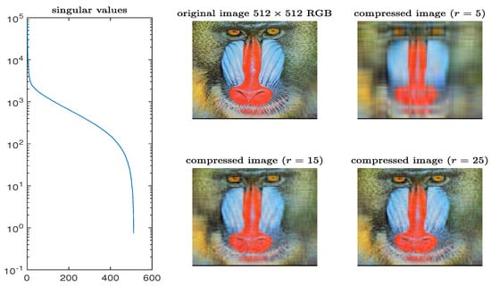
In the matrix context, it is known that just a few singular values suffice to capture the main features of an image, therefore, applying this idea to each one of the three color layers, an RGB image can be approximated by a low tubal rank tensor. Let us consider an image tensor $\mathcal{S}\in {\mathbb{R}}^{n_1\times n_2\times n_3}$ and its c-SVD decomposition $\mathcal{S}=\mathcal{U}{🟉}_c\mathcal{S}{🟉}_c{\mathcal{V}}^T$. Choosing an integer r such as $r\le min(n_1,n_2)$, we can approximate $\mathcal{S}$ by the r tubal rank tensor

$${\displaystyle {\mathcal{S}}_r\approx \sum _{i=1}^r\mathcal{U}(:,i,:){\ast }_c\mathcal{S}(i,i,:){\ast }_c\mathcal{V}{(:,i,:)}^T.}$$

In Figure 1, we represented a $512\times 512$ RGB image and the images obtained for various truncation indices. On the left part, we plotted the singular values of one color layer of the RGB tensor (the exact same behaviour is observed on the two other layers). The rapid decrease of the singular values explain the good quality of compressed images even for small truncation indices.

Applying this idea to our problem, we want to be able to obtain truncated tensor SVDs of the training tensor ${\displaystyle \mathcal{X}}$, without needing to compute the whole c-SVD. After k iterations of the TTGGKA algorithm (for the case $s=1$), we obtain three tensors ${\mathbb{U}}_k\in {\mathbb{R}}^{n_1\times k\times n_3}$, ${\mathbb{V}}_{k+1}\in {\mathbb{R}}^{n_2\times (k+1)\times n_3}$ and ${\tilde{\mathcal{C}}}_k\in {\mathbb{R}}^{(k\times (k+1)\times n_3}$ as defined in Equation (21) such as

$${\mathcal{A}}^T{🟉}_c{\mathbb{U}}_k={\mathbb{V}}_{k+1}{🟉}_c{\tilde{\mathcal{C}}}_k^T.$$

Let ${\displaystyle {\tilde{\mathcal{C}}}_k=\mathsf{\Phi }{🟉}_c\mathsf{\Sigma }{🟉}_c\mathsf{\Psi }}$ the c-SVD of ${\displaystyle {\tilde{\mathcal{C}}}_k}$, noticing that ${\displaystyle {\tilde{\mathcal{C}}}_k\in {\mathbb{R}}^{k\times (k+1)\times n_3}}$ is much smaller than ${\displaystyle \overline{\mathcal{X}}}$. Then first tubal singular values and the left tubal singular tensors of ${\displaystyle \overline{\mathcal{X}}}$ are given by ${\displaystyle \mathsf{\Sigma }(i,i,:)}$ and ${\displaystyle {\mathcal{U}}_k{🟉}_c\mathsf{\Phi }(:,i,:)}$, respectively, for $i\le k$, see [1] for more details.

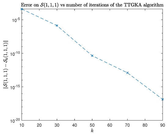
In order to illustrate the ability to approximate the first singular elements of a tensor using the TTGGKA algorithm, we considered a $900\times 900\times 3$ real tensor $\mathcal{A}$ which frontal slices were matrices generated by a finite difference discretization method of differential operators. On Figure 2, we displayed the error on the first diagonal coefficient of the first frontal $\mathcal{S}(1,1,1)$ in function of the number of iteration of the Tensor Tube Golub–Kahan algorithm, where ${\displaystyle \mathcal{A}=\mathcal{U}{🟉}_c\mathcal{S}{🟉}_c{\mathcal{V}}^T}$ is the c-SVD of $\mathcal{A}$.

In

Table 1. ${\parallel \mathcal{S}(i,i,:)-\mathsf{\Sigma }(i,i,:)\parallel }_F$vsk.

	$\mathit{k}=\mathbf{10}$	$\mathit{k}=\mathbf{30}$	$\mathit{k}=\mathbf{50}$	$\mathit{k}=\mathbf{70}$
$\mathcal{S}(1,1,:)$	$3.6\times {10}^{-4}$	$1.3\times {10}^{-5}$	$5.1\times {10}^{-11}$	$4.8\times {10}^{-17}$
$\mathcal{S}(2,2,:)$	$2.0\times {10}^{-3}$	$1.6\times {10}^{-6}$	$5.2\times {10}^{-7}$	$3.1\times {10}^{-8}$
$\mathcal{S}(3,3,:)$	$4.9\times {10}^{-3}$	$5.9\times {10}^{-4}$	$2.3\times {10}^{-4}$	$5.6\times {10}^{-8}$
$\mathcal{S}(4,4,:)$	$8.4\times {10}^{-3}$	$8.8\times {10}^{-4}$	$1.5\times {10}^{-4}$	$1.0\times {10}^{-8}$
$\mathcal{S}(5,5,:)$	$1.4\times {10}^{-2}$	$1.3\times {10}^{-3}$	$2.7\times {10}^{-4}$	$1.1\times {10}^{-8}$

, we reported on the errors on the tensor Frobenius norms of the singular tubes in function of the number k of the Tensor Tube Golub–Kahan algorithm.

The same behaviour was observed on all the other frontal slices. This example illustrate the ability of the TTGKA algorithm for approximating the largest singular tubes.

The projection space is generated by the lateral slices of the tensor $\mathcal{P}={\mathbb{U}}_k{🟉}_c$$\mathsf{\Phi }(:,1:k,:)\in {\mathbb{R}}^{n_1\times i\times n_3}$ derived from the TTGGKA algorithm and the c-SVD decomposition of the bidiagonal tensor ${\displaystyle {\tilde{\mathcal{C}}}_k}$, i.e., the c-linear span of first k lateral slices of $\mathcal{P}$, see [1,19] for more details.

The steps of the Tensor Tubal PCA algorithm for face recognition which finds the closest image in the training database for a given image ${\mathcal{I}}_0$ are summarized in Algorithm 6:

Algorithm 6 The Tensor Tubal PCA algorithm (TTPCA).

1.  Inputs Training Image tensor $\mathcal{X}$ (N images), mean image tensor $\overline{\mathcal{X}}$,Test image ${\mathcal{I}}_0$, index of truncation r, k=number of iterations of the TTGGKA algorithm ($k\ge r$).

2.  Output Closest image in the Training database.

3.  Run k iterations of the TTGGKA algorithm to obtain tensors ${\mathbb{U}}_k$ and $\widehat{{\mathcal{C}}_k}$

4.  Compute $\left[\mathsf{\Phi },\mathsf{\Sigma },\mathsf{\Psi }\right]=$ c-SVD$(\widetilde{{\mathcal{C}}_k})$

5.  Compute the projection tensor ${\mathcal{P}}_r=\left[{\mathcal{P}}_r(:,1,:),\cdots ,{\mathcal{P}}_r(:,r,:)\right]$, where ${\mathcal{P}}_r(:,i,:)={\mathbb{U}}_k{🟉}_c\mathsf{\Phi }(:,i,:)\in {\mathbb{R}}^{n_1\times 1\times n_3}$

6.  Compute the projected Training tensor ${\widehat{\mathcal{X}}}_r={\mathcal{P}}_r^T{🟉}_c\mathcal{X}$ and projected centred test image ${\widehat{\mathcal{I}}}_r={\mathcal{P}}_r^T{🟉}_c(\mathcal{I}-\overline{\mathcal{X}})$

7.  Find $i=arg{min}_{i=1,..,N}{\parallel {\widehat{\mathcal{I}}}_r-{\widehat{\mathcal{X}}}_r(:,i,:)|}_F$

In the next section, we consider image identification problems on various databases.

6. Numerical Tests

In this section, we consider three examples of image identification. In the case of grayscale images, the global version of Golub–Kahan was used to compute the dominant singular values in order to perform a PCA on the data. For the two other situations, we used the Tensor Tubal PCA (TTPCA) method based on the Tube Global Golub–Kahan (TTGGKA) algorithm in order to perform facial recognition on RGB images. The tests were performed with Matlab 2019a, on an Intel i5 laptop with 16 Go of memory. We considered various truncation indices r for which the recognition rates were computed. We also reported the CPU time for the training process.

6.1. Example 1

In this example, we considered the MNIST database of handwritten digits [22]. The database contains two subsets of $28\times 28$ grayscale images (60,000 training images and 10,000 test images). A sample is shown in Figure 3. Each image was vectorized as a vector of length $28\times 28=784$ and, following the process described in Section 3.1, we formed the training and the test matrices of sizes $784\times 60,000$ and $784\times 10,000$, respectively.

Both matrices were centred by substracting the mean training image and the Golub–Kahan algorithm was used to generate an approximation of r dominant singular values $s_i$ and left singular vectors $u_i$, $i=1,\cdots ,r$.

Let us denote ${\mathcal{U}}_r$ the subspace spanned by the columns of $U_r=\left[u_1,\cdots ,u_r\right]$. Let t be a test image and ${\widehat{t}}_r=U_r^{T}t$ its projection onto ${\mathcal{U}}_r$. The closest image in the training dataset is determined by computing

$$i=arg\underset{i=1,..,60,000}{min}\parallel {\widehat{t}}_r-{\widehat{X}}_r(:,i)\parallel ,$$

where ${\widehat{X}}_r={\mathcal{U}}_r^{T}X$.

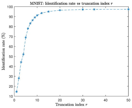
For various truncation indices r, we tested each image of the test subset and computed the recognition rate (i.e., a test is successful if the digit is correctly identified). The results are plotted on Figure 4 and show that a good level of accuracy is obtained with only a few approximate singular values. Due to the large size of the training matrix, it validates the interest of computing only a few singular values with the Golub–Kahan algorithm.

6.2. Example 2

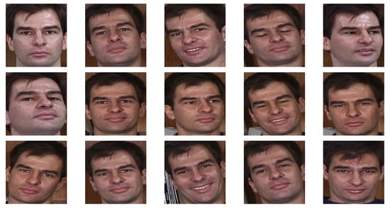
In this example, we used the Georgia Tech database GTDB_ crop [23], which contains 750 face images of 50 persons in different illumination conditions, facial expression and face orientation, as shown in Figure 5. The RGB JPEG images were resized to 100 × 100 × 3 tensors.

Each image file is coded as a $100\times 100\times 3$ tensor and transformed into a 10,000 $\times 1\times 3$ tensor as explained in the previous section. We built the training and test tensors as follows: from 15 pictures of each person in the database, five pictures were randomly chosen and stored in the test folder and the 10 remaining pictures were used for the train tensor. Hence, the database was partitioned into two subsets containing 250 and 500 items, respectively, at each iteration of the simulation.

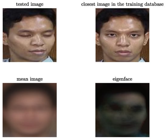
We applied the TTGGKA based Algoritm 6 for various truncation indices. In Figure 6, we represented a test image (top left position), the closest image in the database (top right), the mean image of the training database (bottom left) and the eigenface associated to the test image (bottom right).

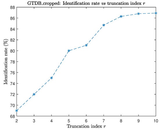
In order compute the rate of recognition, we ran 100 simulations, obtained the number of successes (i.e., a test is successful if the person is correctly identified) and reported the best identification rates, in function of the truncation index r in Figure 7.

The results match the performances observed in the literature [24] for this database and it confirms that the use of a Golub–Kahan strategy is interesting especially because, in terms of training, the Tube Tensor PCA algorithm required only 5 s instead of 25 s when using a c-SVD.

6.3. Example 3

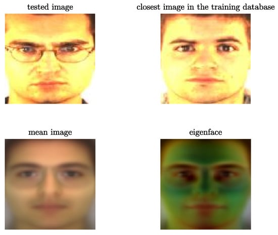
In the second example, we used the larger AR face database (cropped version) (Face crops) [9], which contains 2600 bitmap pictures of human faces (50 males and 50 females, 26 pictures per person), with different expressions, lightning conditions, facial expressions and face orientation. The bitmap pictures were resized to 100 × 100 Jpeg images. The same protocol as for Example 1 was followed: we partitioned the set of images in two subsets. Out of 26 pictures, 6 pictures were randomly chosen as test images and the remaining 20 were put into the training folder. The training process took 24 s while it would have taken 81.5 s if using a c-SVD. An example of test image, the closest match in the dataset, the mean image and its associated eigenface are shown in Figure 8.

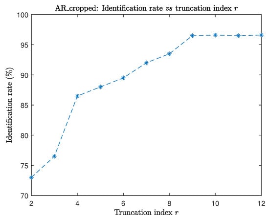
We applied our approach (TTPCA) to the 10,000 $\times 2000\times 3$ training tensor $\mathcal{X}$ and plotted the recognition rate as a function of the truncation index in Figure 9.

For all examples, it is worth noticing that, as expected in face identification problems, only a few of the first largest singular elements suffice to capture the main features of an image. Therefore, the Golub–Kahan based strategies such as the TTPCA method are an interesting choice.

7. Conclusions

In this manuscript, we focused on two types of Golub–Kahan factorizations. We used the recent advances in the field of tensor factorization and showed that this approach is efficient for image identification. The main feature of this approach resides in the ability of the Global Golub–Kahan algorithms to approximate the dominant singular elements of a training matrix or tensor without needing to compute the SVD. This is particularly important as the matrices and tensors involved in this type of application can be very large. Moreover, in the case for which color has to be taken into account, this approach do not involve a conversion to grayscale, which can be very important for some applications. In a future work, we would like to study the feasability of implementing the promising randomized PCA approaches in the Golub–Kahan tensor algorithm in order to improve the training process computational cost in the case of very large datasets.

References

- Kilmer, M.E.; Braman, K.; Hao, N.; Hoover, R.C. Third-order tensors as operators on matrices: A theoretical and computational framework with applications in imaging. SIAM J. Matrix Anal. Appl. 2013, 34, 148–172. [Google Scholar]
- Kolda, T.G.; Bader, B.W. Tensor Decompositions and Applications. SIAM Rev. 2009, 3, 455–500. [Google Scholar] [CrossRef]
- Zhang, J.; Saibaba, A.K.; Kilmer, M.E.; Aeron, S. A randomized tensor singular value decomposition based on the t-product. Numer Linear Algebra Appl. 2018, 25, e2179. [Google Scholar] [CrossRef]
- Cai, S.; Luo, Q.; Yang, M.; Li, W.; Xiao, M. Tensor robust principal component analysis via non-convex low rank approximation. Appl. Sci. 2019, 9, 1411. [Google Scholar] [CrossRef]
- Kong, H.; Xie, X.; Lin, Z. t-Schatten-p norm for low-rank tensor recovery. IEEE J. Sel. Top. Signal Process. 2018, 12, 1405–1419. [Google Scholar] [CrossRef]
- Lin, Z.; Chen, M.; Ma, Y. The augmented Lagrange multiplier method for exact recovery of corrupted low-rank matrices. arXiv 2010, arXiv:1009.5055. [Google Scholar]
- Kang, Z.; Peng, C.; Cheng, Q. Robust PCA via nonconvex rank approximation. In Proceedings of the 2015 IEEE International Conference on Data Mining, Atlantic City, NJ, USA, 14–17 November 2015. [Google Scholar]
- Lu, C.; Feng, J.; Chen, Y.; Liu, W.; Lin, Z.; Yan, S. Tensor Robust Principal Component Analysis with a New Tensor Nuclear Norm. IEEE Anal. Mach. Intell. 2020, 42, 925–938. [Google Scholar] [CrossRef] [PubMed]
- Martinez, A.M.; Kak, A.C. PCA versus LDA. IEEE Trans. Pattern Anal. Mach. Intell. 2001, 23, 228–233. [Google Scholar] [CrossRef]
- Guide, M.E.; Ichi, A.E.; Jbilou, K.; Sadaka, R. Tensor Krylov subspace methods via the T-product for color image processing. arXiv 2020, arXiv:2006.07133. [Google Scholar]
- Brazell, M.; Navasca, N.L.C.; Tamon, C. Solving Multilinear Systems Via Tensor Inversion. SIAM J. Matrix Anal. Appl. 2013, 34, 542–570. [Google Scholar] [CrossRef]
- Beik, F.P.A.; Jbilou, K.; Najafi-Kalyani, M.; Reichel, L. Golub–Kahan bidiagonalization for ill-conditioned tensor equations with applications. Numer. Algorithms 2020, 84, 1535–1563. [Google Scholar] [CrossRef]
- Ichi, A.E.; Jbilou, K.; Sadaka, R. On some tensor tubal-Krylov subspace methods via the T-product. arXiv 2020, arXiv:2010.14063. [Google Scholar]
- Guide, M.E.; Ichi, A.E.; Jbilou, K. Discrete cosine transform LSQR and GMRES methods for multidimensional ill-posed problems. arXiv 2020, arXiv:2103.11847. [Google Scholar]
- Vasilescu, M.A.O.; Terzopoulos, D. Multilinear image analysis for facial recognition. In Proceedings of the Object Recognition Supported by User Interaction for Service Robots, Quebec City, QC, Canada, 11–15 August 2002; pp. 511–514. [Google Scholar]
- Jain, A. Fundamentals of Digital Image Processing; Prentice–Hall: Englewood Cliffs, NJ, USA, 1989. [Google Scholar]
- Ng, M.K.; Chan, R.H.; Tang, W. A fast algorithm for deblurring models with Neumann boundary conditions. SIAM J. Sci. Comput. 1999, 21, 851–866. [Google Scholar] [CrossRef]
- Kernfeld, E.; Kilmer, M.; Aeron, S. Tensor-tensor products with invertible linear transforms. Linear Algebra Appl. 2015, 485, 545–570. [Google Scholar] [CrossRef]
- Kilmer, M.E.; Martin, C.D. Factorization strategies for third-order tensors. Linear Algebra Appl. 2011, 435, 641–658. [Google Scholar] [CrossRef]
- Golub, G.H.; Van Loan, C.F. Matrix Computations, 3rd ed.; Johns Hopkins University Press: Baltimore, MD, USA, 1996. [Google Scholar]
- Savas, B.; Eldén, L. Krylov-type methods for tensor computations I. Linear Algebra Appl. 2013, 438, 891–918. [Google Scholar] [CrossRef]
- Lecun, Y.; Cortes, C.; Curges, C. The MNIST Database. Available online: http://yann.lecun.com/exdb/mnist/ (accessed on 22 February 2021).
- Nefian, A.V. Georgia Tech Face Database. Available online: http://www.anefian.com/research/face_reco.htm (accessed on 22 February 2021).
- Wang, S.; Sun, M.; Chen, Y.; Pang, E.; Zhou, C. STPCA: Sparse tensor Principal Component Analysis for feature extraction. In Proceedings of the 21st International Conference on Pattern Recognition (ICPR2012), Tsukuba, Japan, 11–15 November 2012; pp. 2278–2281. [Google Scholar]
Publisher’s Note: MDPI stays neutral with regard to jurisdictional claims in published maps and institutional affiliations. |
© 2021 by the authors. Licensee MDPI, Basel, Switzerland. This article is an open access article distributed under the terms and conditions of the Creative Commons Attribution (CC BY) license (https://creativecommons.org/licenses/by/4.0/).