Dynamics of Stage-Structured Predator–Prey Model with Beddington–DeAngelis Functional Response and Harvesting

Abstract

In this paper, we investigate the stability of equilibrium in the stage-structured and density-dependent predator–prey system with Beddington–DeAngelis functional response. First, by checking the sign of the real part for eigenvalue, local stability of origin equilibrium and boundary equilibrium are studied. Second, we explore the local stability of the positive equilibrium for $\tau =0$ and $\tau \ne 0$ (time delay $\tau$ is the time taken from immaturity to maturity predator), which shows that local stability of the positive equilibrium is dependent on parameter $\tau$. Third, we qualitatively analyze global asymptotical stability of the positive equilibrium. Based on stability theory of periodic solutions, global asymptotical stability of the positive equilibrium is obtained when $\tau =0$; by constructing Lyapunov functions, we conclude that the positive equilibrium is also globally asymptotically stable when $\tau \ne 0$. Finally, examples with numerical simulations are given to illustrate the obtained results.

1. Introduction

The dynamical behavior of the predator–prey system is one of the main research topics in mathematical ecology and theoretical biology [1,2,3,4,5,6,7,8,9]. Functional response is the core component of the community and food web model, and their mathematical form strongly affects the dynamics and stability of the ecosystem [10,11,12,13,14]. Beddington [15] and DeAngelis [16] originally proposed the predator–prey model as follows:

$$\left\{\begin{array}{c}\frac{dx\left(t\right)}{dt}=x\left(t\right)\left(a-bx\left(t\right)-\frac{cy\left(t\right)}{m_1+m_{2}x\left(t\right)+m_{3}y\left(t\right)}\right),\hfill \\ \frac{dy\left(t\right)}{dt}=y\left(t\right)\left(-d+\frac{fx\left(t\right)}{m_1+m_{2}x\left(t\right)+m_{3}y\left(t\right)}\right),\hfill \end{array}\right.$$

(1)

where $x\left(t\right)$ is the prey density, $y\left(t\right)$ is the predator density, a is the intrinsic growth rate of the prey, b represents the intensity of intraspecific competition of the prey, and d represents the predator’s death rate. The Beddington–DeAngelis functional response is similar to the well-known Holling II type [17,18] functional response, but it has an extra term $m_{3}y$ in the denominator modeling mutual interference among predators.

The functional response of consumers is a function of resource density [17,19,20]. However, it has been shown that other species and other predators can alter the predation process directly or indirectly [21]. In addition, Kratina [21] showed that predator dependence is very important not only when the predator density on per capita predation rate is very high, but also when the predator density is low. Therefore, we need to consider the realistic level of predator density when we study the predator–prey system.

Moreover, in nature, many species undergo two stages [22,23]: immature and mature, and species at these two stages may have different behaviors. The model of single-species stage-structured dynamics [22] was described as

$$\begin{array}{c}\frac{d{x}_1\left(t\right)}{dt}=d{x}_2\left(t\right)-d_i{x}_1\left(t\right)-d{e}^{-d_i\tau }{x}_2(t-\tau ),\hfill \\ \frac{d{x}_2\left(t\right)}{dt}=d{e}^{-d_i\tau }{x}_2(t-\tau )-r{x}_2^2\left(t\right),\hfill \end{array}$$

(2)

where $x_1\left(t\right)$ and $x_2\left(t\right)$ represent the immature and mature populations densities, respectively, and $\tau$ represents a constant time to maturity. Therefore, in order to be in accord with the natural phenomenon, the system with the stage structure recently has been extensively studied [24,25,26,27,28,29,30]. Liu and Beretta [27] studied time delay $\tau$ in the response term $\frac{x\left(t\right)}{m_1+m_{2}x\left(t\right)+m_{3}y\left(t\right)}$ of (1) in the predator equation, that is,

$$\left\{\begin{array}{c}\frac{dx\left(t\right)}{dt}=rx\left(t\right)\left(1-\frac{x\left(t\right)}{K}\right)-\frac{gx\left(t\right)y\left(t\right)}{1+k_{1}x\left(t\right)+k_{2}y\left(t\right)},\hfill \\ \frac{dy\left(t\right)}{dt}=-dy\left(t\right)+\frac{ng{e}^{-d_j\tau }x(t-\tau )y(t-\tau )}{1+k_{1}x(t-\tau )+k_{2}y(t-\tau )},\hfill \\ \frac{d{y}_i\left(t\right)}{dt}=\frac{ngx\left(t\right)y\left(t\right)}{1+k_{1}x\left(t\right)+k_{2}y\left(t\right)}-\frac{ng{e}^{-d_j\tau }x(t-\tau )y(t-\tau )}{1+k_{1}x(t-\tau )+k_{2}y(t-\tau )}-d_j{y}_j\left(t\right),\hfill \end{array}\right.$$

(3)

where $g>0$ (units: 1/time) and $k_1>0$ (units: 1/prey) stand the effects of capture rate and handling time, respectively, on the feeding rate; n is the birth rate of the predator; and $k_2\ge 0$ (units: 1/predator) stands the magnitude of interference among predators. Liu and Beretta [27] pointed out the difference between Beddington–DeAngelis functional response and Holling type II, and the effect of $k_{2}y$ (describing mutual interference by predators) on the dynamic of the system (3).

On the basis of the system (1) and the system (2), She and Li [29] investigated a predator–prey system with density-dependence for predator and stage structure for prey

$$\left\{\begin{array}{c}{x}_i^{\prime }\left(t\right)=a^{\prime }x\left(t\right)-d_i{x}_i\left(t\right)-a^{\prime }{e}^{-d_i\tau }x(t-\tau ),\hfill \\ x^{\prime }\left(t\right)=a^{\prime }{e}^{-d_i\tau }x(t-\tau )-b{x}^2\left(t\right)-\frac{cx\left(t\right)y\left(t\right)}{m_1+m_{2}x\left(t\right)+m_{3}y\left(t\right)},\hfill \\ y^{\prime }\left(t\right)=-dy\left(t\right)-p{y}^2\left(t\right)+\frac{cx\left(t\right)y\left(t\right)}{m_1+m_{2}x\left(t\right)+m_{3}y\left(t\right)},\hfill \end{array}\right.$$

(4)

where p stands for predator density-dependent mortality rate, the predator consumes prey with functional response of Beddington-DeAngelis type $\frac{cx\left(t\right)y\left(t\right)}{m_1+m_{2}x\left(t\right)+m_{3}y\left(t\right)}$ and contributes to its growth with rate $\frac{fx\left(t\right)y\left(t\right)}{m_1+m_{2}x\left(t\right)+m_{3}y\left(t\right)}$. Note that compared with the system (1), the system (4) contains not only $b{x}^2\left(t\right)$ (which stands for intraspecific competition of prey species), but also $p{y}^2\left(t\right)$ (which stands for intraspecific competition of predator species). That is, they consider both the prey density dependence and the predator density dependence in the predator–prey model (4). She and Li [29] studied the dynamics of the system (4) and pointed out the impact of the predator density-dependent mortality rate p on the global attraction and permanence of the system (4).

The development of biological resources, the management of renewable resources, and the harvest of populations are universal human purposes for realizing the economic benefits of fishery, forestry and wildlife management [31,32]. Many researchers [28,30,33,34] have extensively studied the predator–prey model with harvesting and the role of harvesting in renewable resource management. Brauer [35] introduced the predator–prey system with constant-rate prey harvesting

$$x^{\prime }=xf(x,y)-F,y^{\prime }=yg(x,y),$$

(5)

where prey is harvested at a constant time rate F. May [36] put forward two types of harvesting regimes: constant-yield harvesting (representing harvested biomass independent of the size of the population) and constant-effort harvesting (representing harvested biomass proportional to the size of the population).

Based on the system (3), we construct a density-dependent and constant-effort harvesting predator–prey model:

$$\left\{\begin{array}{c}\frac{dx\left(t\right)}{dt}=x\left(t\right)\left(a-bx\left(t\right)-\frac{cy\left(t\right)}{m_1+m_{2}x\left(t\right)+m_{3}y\left(t\right)}\right)-E_{1}x\left(t\right),\hfill \\ \frac{dy\left(t\right)}{dt}=-dy\left(t\right)-p{y}^2\left(t\right)+\frac{f{e}^{-d_i\tau }x(t-\tau )y(t-\tau )}{m_1+m_{2}x(t-\tau )+m_{3}y(t-\tau )}-E_{2}y\left(t\right),\hfill \\ \frac{d{y}_i\left(t\right)}{dt}=-d_i{y}_i\left(t\right)-p{y}^2\left(t\right)+\frac{fx\left(t\right)y\left(t\right)}{m_1+m_{2}x\left(t\right)+m_{3}y\left(t\right)}+p{e}^{-d_i\tau }{y}^2(t-\tau )\hfill \\ -\frac{f{e}^{-d_i\tau }x(t-\tau )y(t-\tau )}{m_1+m_{2}x(t-\tau )+m_{3}y(t-\tau )},\hfill \end{array}\right.$$

(6)

where $y_i\left(t\right)$ denotes the immature or juvenile predator density, juveniles suffer a mortality rate $d_i$ and take $\tau$ units of time to be mature and $e^{-d_i\tau }$ is the surviving rate of each immature predator to reach maturity. $E_1$ and $E_2$ denote the harvesting effort of the mature population of prey and predator, respectively. Further, all the parameters a, $d_i$, b, c, d, f, $m_1$, $m_2$, $m_3$, p, $E_1$, $E_2$, and $\tau$ are positive.

In the system (6), as $y_i\left(t\right)$ does not intervene in the dynamics of $x\left(t\right)$ and $y\left(t\right)$, system (6) is equal to the following system:

$$\left\{\begin{array}{c}\frac{dx\left(t\right)}{dt}=x\left(t\right)\left(a-bx\left(t\right)-\frac{cy\left(t\right)}{m_1+m_{2}x\left(t\right)+m_{3}y\left(t\right)}\right)-E_{1}x\left(t\right),\hfill \\ \frac{dy\left(t\right)}{dt}=-dy\left(t\right)-p{y}^2\left(t\right)+\frac{f{e}^{-d_i\tau }x(t-\tau )y(t-\tau )}{m_1+m_{2}x(t-\tau )+m_{3}y(t-\tau )}-E_{2}y\left(t\right).\hfill \end{array}\right.$$

(7)

The initial conditions of the system (7) is

$$x_0\left(\theta \right)={\varphi }_1\left(\theta \right)\ge 0,y_0\left(\theta \right)={\varphi }_2\left(\theta \right)\ge 0,\theta \in [-\tau ,0],x\left(0\right)>0,y\left(0\right)>0,$$

(8)

where $\varphi =({\varphi }_1,{\varphi }_2)\in C([-\tau ,0],R_{+}^2),R_{+}^2=\{(x,y):x\ge 0,y\ge 0\}$, $\Vert \varphi \Vert =max\left\{\right|\varphi \left(\theta \right)|:\theta \in [-\tau ,0\left]\right\}$, and $\left|\varphi \right|$ is the modulus in $R_{+}^2$. Normally, we use notation $x_t\left(\theta \right)=x(t+\theta ),\theta \in [-\tau ,0]$.

This paper mainly investigates the local and global stability of positive equilibrium in the system (7) on parameter $\tau$, which is organized as follows. In Section 2, we study local stability of origin equilibrium and boundary equilibrium. In Section 3, we derive local stability of the positive equilibrium for $\tau =0$ and $\tau \ne 0$, respectively. In Section 4, we obtain the global asymptotical stability of the positive equilibrium for $\tau =0$ and $\tau \ne 0$, respectively. Last, we conclude the paper.

2. Local Stability of Origin Equilibrium and Boundary Equilibrium

For any value of all parameters, system (7) has the equilibria $E_0(0,0)$ and $E_1\left(\frac{a-E_1}{b},0\right)$, denoted as the origin and the boundary equilibrium, respectively. In the following, we determine the local stability of two equilibria by the sign of eigenvalue for the corresponding characteristic matrix.

First, for origin equilibrium $E_0$, the corresponding characteristic matrix is

$$J_{(0,0)}=\left[\begin{array}{cc}\lambda -a+E_1& 0\\ 0& \lambda +d+E_2\end{array}\right],$$

and the eigenvalues are

$${\lambda }_1=a-E_1>0,{\lambda }_2=-(d+E_2)<0.$$

Clearly, $E_0(0,0)$ is hyperbolic saddle and is unstable.

Next, for boundary equilibrium $E_1$, the corresponding characteristic matrix is

$$J_{\left(\frac{a-E_1}{b},0\right)}=\left[\begin{array}{cc}\lambda +a-E_1& \frac{c(a-E_1)}{b{m}_1+m_2(a-E_1)}\\ 0& \lambda +d+E_2-\frac{(a-E_1)f{e}^{-(\lambda +d_i)\tau }}{b{m}_1+m_2(a-E_1)}\end{array}\right].$$

We can obtain one eigenvalue ${\lambda }_1=-(a-E_1)<0$, the second eigenvalue is determined by the following equation:

$${\lambda }_2+d+E_2-\frac{(a-E_1)f{e}^{-({\lambda }_2+d_i)\tau }}{b{m}_1+m_2(a-E_1)}=0.$$

Let n be the independent variable and g be the dependent variable; then, the straight line $g=n+(d+E_2)$ and the curve $g=\frac{(a-E_1)f{e}^{-d_i\tau }}{b{m}_1+m_2(a-E_1)}{e}^{-n\tau }$ must intersect at a unique point $({\lambda }_2,g)$. Further, we can get the following:

(i)

if $d+E_2>\frac{(a-E_1)f{e}^{-d_i\tau }}{b{m}_1+m_2(a-E_1)}$, then ${\lambda }_2<0$;

(ii)

if $d+E_2<\frac{(a-E_1)f{e}^{-d_i\tau }}{b{m}_1+m_2(a-E_1)}$, then ${\lambda }_2>0$;

(ii)

if $d+E_2=\frac{(a-E_1)f{e}^{-d_i\tau }}{b{m}_1+m_2(a-E_1)}$, then ${\lambda }_2=0$.

Therefore, we have the following conclusion about local stability of boundary equilibrium.

Theorem 1. 

 

(1) If $(a-E_1)\left[f{e}^{-d_i\tau }-(d+E_2)m_2\right]<b{m}_1(d+E_2)$, boundary equilibrium $\left(\frac{a-E_1}{b},0\right)$ is locally asymptotically stable;

(2) If $(a-E_1)\left[f{e}^{-d_i\tau }-(d+E_2)m_2\right]>b{m}_1(d+E_2)$, boundary equilibrium $\left(\frac{a-E_1}{b},0\right)$ is unstable;

(3) If $(a-E_1)\left[f{e}^{-d_i\tau }-(d+E_2)m_2\right]=b{m}_1(d+E_2)$, boundary equilibrium $\left(\frac{a-E_1}{b},0\right)$ is linearly neutrally stable.

Remark 1. 

By Theorem 1, when $\tau >{\tau }^{*}$, $\left(\frac{a-E_1}{b},0\right)$ is locally asymptotically stable; when $\tau <{\tau }^{*}$, $\left(\frac{a-E_1}{b},0\right)$ is unstable; when $\tau ={\tau }^{*}$, $\left(\frac{a-E_1}{b},0\right)$ is linearly neutrally stable, where

$${\tau }^{*}=\frac{1}{d_i}log\frac{f(a-E_1)}{(d+E_2)[b{m}_1+m_2(a-E_1)]}.$$

That is, ${\tau }^{*}$ is a threshold for the stability of the boundary equilibrium.

3. Local Stability of the Positive Equilibrium

We denote $(x^{*},y^{*})$ as equilibrium other than the origin equilibrium and boundary equilibrium for the system (7) and satisfying the algebraic equations

$$\left\{\begin{array}{c}a-b{x}^{*}-\frac{c{y}^{*}}{m_1+m_2{x}^{*}+m_3{y}^{*}}-E_1=0,\hfill \\ -d-p{y}^{*}+\frac{f{e}^{-d_i\tau }{x}^{*}}{m_1+m_2{x}^{*}+m_3{y}^{*}}-E_2=0.\hfill \end{array}\right.$$

(9)

From $a-bx-\frac{cy}{m_1+m_{2}x+m_{3}y}-E_1=0$, we have the curve

$$y=\frac{b{m}_2{x}^2+[b{m}_1-(a-E_1)m_2]x-(a-E_1)m_1}{(a-E_1)m_3-c-b{m}_{3}x}=F\left(x\right);$$

by $-d-py+\frac{f{e}^{-d_i\tau }x}{m_1+m_{2}x+m_{3}y}-E_2=0$, we have another curve

$$x=\frac{p{m}_3{y}^2+[p{m}_1+(d+E_2)m_3]y+(d+E_2)m_1}{f{e}^{-d_i\tau }-(d+E_2)m_2-p{m}_{2}y}=H\left(y\right).$$

By considering the intersection of curves $y=F\left(x\right)$ and $x=H\left(y\right)$ in the first quadrant, we can obtain if the condition

$$(a-E_1)\left[f{e}^{-d_i\tau }-(d+E_2)m_2\right]>b{m}_1(d+E_2)$$

(10)

holds, $(x^{*},y^{*})$ is a positive equilibrium of system (7).

By the condition (10), we can directly obtain the following result.

Remark 2. 

The positive equilibrium $(x^{*},y^{*})$ exists for any predation maturation time τ in the interval $[0,{\tau }^{*})$.

The Jacobian matrix [37] of differential system (7) with delay coefficients at $(x^{*},y^{*})$ is

$$J_{(x^{*},y^{*})}=\left[\begin{array}{cc}a-E_1-2b{x}^{*}-\frac{c{y}^{*}(m_1+m_3{y}^{*})}{{(m_1+m_2{x}^{*}+m_3{y}^{*})}^2}& -\frac{c{x}^{*}(m_1+m_2{x}^{*})}{{(m_1+m_2{x}^{*}+m_3{y}^{*})}^2}\\ \frac{f{e}^{-d_i\tau }{y}^{*}(m_1+m_3{y}^{*})}{{(m_1+m_2{x}^{*}+m_3{y}^{*})}^2}{e}^{-\lambda \tau }& -(d+E_2)-2p{y}^{*}+\frac{f{e}^{-d_i\tau }{x}^{*}(m_1+m_2{x}^{*})}{{(m_1+m_2{x}^{*}+m_3{y}^{*})}^2}{e}^{-\lambda \tau }\end{array}\right].$$

Therefore, the characteristic equation is

$${\lambda }^2+a_1\left(\tau \right)\lambda +a_2\left(\tau \right)\lambda e^{-\lambda \tau }+a_3\left(\tau \right)e^{-\lambda \tau }+a_4\left(\tau \right)=0,$$

(11)

where

$$a_1\left(\tau \right)=d+2p{y}^{*}+E_2+(E_1-a)+2b{x}^{*}+\frac{c{y}^{*}(m_1+m_3{y}^{*})}{{(m_1+m_2{x}^{*}+m_3{y}^{*})}^2},$$

$$a_2\left(\tau \right)=-\frac{f{e}^{-d_i\tau }{x}^{*}(m_1+m_2{x}^{*})}{{(m_1+m_2{x}^{*}+m_3{y}^{*})}^2},a_3\left(\tau \right)=(a-2b{x}^{*}-E_1)\frac{f{e}^{-d_i\tau }{x}^{*}(m_1+m_2{x}^{*})}{{(m_1+m_2{x}^{*}+m_3{y}^{*})}^2},$$

$$a_4\left(\tau \right)=(d+2p{y}^{*}+E_2)\left(E_1-a+2b{x}^{*}+\frac{c{y}^{*}(m_1+m_3{y}^{*})}{{(m_1+m_2{x}^{*}+m_3{y}^{*})}^2}\right).$$

We noticed that if $x^{*}>\frac{a-E_1}{2b}$, then $a_3\left(\tau \right)+a_4\left(\tau \right)>0$. Therefore, when $x^{*}>\frac{a-E_1}{2b}$, $\lambda =0$ cannot be a characteristic root of Equation (11).

The parameter $\tau$ is the time from immature to mature predator. Time delay $\tau \ne 0$, it shows the predator population is divided into immature and mature; time delay $\tau =0$, it shows the model does not consider the immature predators. In the following, we discuss the local stability of positive equilibrium $(x^{*},y^{*})$ for $\tau =0$ and $\tau \ne 0$, respectively.

3.1. Local Stability of the Positive Equilibrium for $\tau =0$

When $\tau =0$, characteristic Equation (11) becomes

$${\lambda }^2+[a_1\left(0\right)+a_2\left(0\right)]\lambda +a_3\left(0\right)+a_4\left(0\right)=0.$$

(12)

Obviously, when $\left\{\begin{array}{c}{a}_1\left(0\right)+a_2\left(0\right)>0\hfill \\ a_3\left(0\right)+a_4\left(0\right)>0\hfill \end{array}\right.$, all roots of characteristic Equation (12) have negative real part. Therefore, $(x^{*}\left(0\right),y^{*}\left(0\right))$ is locally asymptotically stable.

Further, by

$$a_1\left(0\right)+a_2\left(0\right)=b{x}^{*}\left(0\right)+p{y}^{*}\left(0\right)+\frac{(f{m}_3-c{m}_2)x^{*}\left(0\right)y^{*}\left(0\right)}{{(m_1+m_2{x}^{*}\left(0\right)+m_3{y}^{*}\left(0\right))}^2},$$

we can obtain that if $f{m}_3\ge c{m}_2$, then $a_1\left(0\right)+a_2\left(0\right)>0$. According to the previous analysis, we also have if $x^{*}>\frac{a-E_1}{2b}$, $a_3\left(0\right)+a_4\left(0\right)>0$. Therefore, we get the following conclusion.

Theorem 2. 

Let $(x^{*},y^{*})$ is a positive equilibrium of system (7), if the inequality (10) and the following inequalities

$$\left\{\begin{array}{c}{x}^{*}>\frac{a-E_1}{2b}\hfill \\ c{m}_2\le f{m}_3\hfill \end{array}\right.$$

(13)

hold, the positive equilibrium $(x^{*},y^{*})$ of system (7) is locally asymptotically stable for $\tau =0$.

Example 1. 

Let $a=3$, $b=2$, $c=2$, $d=0.1$, $p=10$, $f=12$, $m_1=\frac{1}{8}$, $m_2=4$, $m_3=2$, $E_1=0.5$, $E_2=0.05$, and $\tau =0$, the system (7) becomes

$$\left\{\begin{array}{c}\frac{dx\left(t\right)}{dt}=x\left(3-2x-\frac{2y}{\frac{1}{8}+4x+2y}\right)-0.5x,\hfill \\ \frac{dy\left(t\right)}{dt}=-0.1y-10y^2+\frac{12xy}{\frac{1}{8}+4x+2y}-0.05y.\hfill \end{array}\right.$$

(14)

Clearly, $(a-E_1)(f{e}^{-d_i\tau }-(d+E_2)m_2)-b(d+E_2)m_1=28.4625>0$. Therefore, the system (14) exists a positive equilibrium. Moreover, we obtain the positive equilibrium $(1.2040,0.2505)$ of system (14). As $\frac{a-E_1}{2b}=0.625<1.2040$ and $c{m}_2-f{m}_3=-16<0$, the equilibrium $(1.2040,0.2505)$ is locally asymptotically stable by Theorem 2.

3.2. Local Stability of the Positive Equilibrium for $\tau \ne 0$

In this subsection, we further discuss the sign of the real part of the characteristic root for the characteristic Equation (11) with the change of parameter $\tau$, and determine stability switch.

First, assume that characteristic Equation (11) has a characteristic root with zero real part, and let it be $\lambda =i\omega (\omega \in R$ and $\omega \ne 0)$. Putting it into the characteristic Equation (11), we have

$$\left\{\begin{array}{c}{a}_2\omega sin\omega \tau +a_{3}cos\omega \tau ={\omega }^2-a_4,\hfill \\ a_2\omega cos\omega \tau -a_{3}sin\omega \tau =-a_1\omega .\hfill \end{array}\right.$$

(15)

Here, $a_1\left(\tau \right)$, $a_2\left(\tau \right)$, $a_3\left(\tau \right)$ and $a_4\left(\tau \right)$ are abbreviated as $a_1$, $a_2$, $a_3$ and $a_4$, respectively. From Equation (15), we can get

$${\omega }^4+(a_1^2-a_2^2-2a_4){\omega }^2+a_4^2-a_3^2=0.$$

(16)

Regarding ${\omega }^2$ as an invariant, by the quadratic root formula, we have

$${\omega }_{\pm }^2=\frac{(a_2^2+2a_4-a_1^2)\pm \sqrt{{(a_1^2-a_2^2-2a_4)}^2-4(a_4^2-a_3^2)}}{2}.$$

(17)

We discuss the case of roots for the Equation (16):

(I) If

$$\left\{\begin{array}{c}{a}_1^2-a_2^2-2a_4>0,\hfill \\ a_4^2-a_3^2>0,\hfill \\ {(a_1^2-a_2^2-2a_4)}^2-4(a_4^2-a_3^2)>0\hfill \end{array}\right.$$

(18)

${\omega }_{+}^2$ and ${\omega }_{-}^2$ are negative, which obviously contradicts with $\omega \in R$. Therefore, Equation (16) does not have real roots, that is, characteristic Equation (11) does not have purely imaginary roots. Moreover, if the conditions (10) and (13) hold, all roots of the characteristic Equation (12) have negative real part for $\tau =0$. Therefore, by Rouche’s theorem, it follows that the roots of the characteristic Equation (11) also have negative real part.

(II) If

$$\left\{\begin{array}{c}{a}_4^2-a_3^2<0,\hfill \\ or\hfill \\ a_1^2-a_2^2-2a_4<0,{(a_1^2-a_2^2-2a_4)}^2-4(a_4^2-a_3^2)=0,\hfill \end{array}\right.$$

(19)

Equation (16) has a positive root ${\omega }_0^2$. Furthermore, putting ${\omega }_0^2$ into Equations (15), we have

$${\tau }_n=\frac{1}{{\omega }_0}arcsin\left\{\frac{a_2{\omega }_0({\omega }_0^2-a_4)+a_1{a}_3{\omega }_0}{a_2^2{\omega }_0^2+a_3^2}\right\}+\frac{2n\pi }{{\omega }_0},n=0,1,2,\cdots .$$

(20)

(III) If

$$\left\{\begin{array}{c}{a}_4^2-a_3^2>0,\hfill \\ a_1^2-a_2^2-2a_4<0,\hfill \\ {(a_1^2-a_2^2-2a_4)}^2-4(a_4^2-a_3^2)>0,\hfill \end{array}\right.$$

(21)

Equation (16) has two positive roots ${\omega }_{\pm }^2$. Putting ${\omega }_{\pm }^2$ into Equations (15), we obtain

$${\tau }_j^{\pm }=\frac{1}{{\omega }_{\pm }}arcsin\left\{\frac{a_2{\omega }_{\pm }({\omega }_{\pm }^2-a_4)+a_1{a}_3{\omega }_{\pm }}{a_2^2{\omega }_{\pm }^2+a_3^2}\right\}+\frac{2j\pi }{{\omega }_{\pm }},j=0,1,2,\cdots .$$

(22)

From the above analysis, we have the following conclusion.

Theorem 3. 

 

(i) If conditions (10) and (19) hold and $\tau ={\tau }_n$, then characteristic Equation (11) has a pair of purely imaginary roots $\pm i{\omega }_0$.

(ii) If conditions (10) and (21) hold and $\tau ={\tau }_j^{+}$($\tau ={\tau }_j^{-}$), then characteristic Equation (11) has a pair of purely imaginary roots $\pm i{\omega }_{+}$($\pm i{\omega }_{-}$).

Second, we have that when $\tau >{\tau }_0$, $\tau >{\tau }_j^{+}$, and $\tau <{\tau }_j^{-}$, there are roots with positive real part in the characteristic Equation (11). Let these characteristic roots with positive real part be

$${\lambda }_0={\alpha }_0\left(\tau \right)+i{\omega }_0\left(\tau \right),{\lambda }_j^{\pm }={\alpha }_j^{\pm }\left(\tau \right)+i{\omega }_j^{\pm }\left(\tau \right),j=0,1,2,\cdots ,$$

and

$${\alpha }_0\left({\tau }_0\right)=0,{\omega }_0\left({\tau }_0\right)={\omega }_0,{\alpha }_j^{\pm }\left({\tau }_j^{\pm }\right)=0,{\omega }_j^{\pm }\left({\tau }_j^{\pm }\right)={\omega }_{\pm },$$

where

$${\tau }_0=\frac{1}{{\omega }_0}arcsin\left\{\frac{a_2{\omega }_0({\omega }_0^2-a_4)+a_1{a}_3{\omega }_0}{a_2^2{\omega }_0^2+a_3^2}\right\}.$$

According to the characteristic Equation (11), we get

$$\frac{d\lambda }{d\tau }=-\frac{\lambda ({\lambda }^2+a_1\lambda +a_4)}{2\lambda +a_1+a_2{e}^{-\lambda \tau }+\tau ({\lambda }^2+a_1\lambda +a_4)}.$$

(23)

Obviously, $sign\left\{\frac{d}{d\tau }Re\lambda \left(\tau \right)\right\}=sign\left\{Re{\left(\frac{d\lambda \left(\tau \right)}{d\tau }\right)}^{-1}\right\}$. Therefore, in order to judge the sign of $\frac{d}{d\tau }Re\lambda \left(\tau \right)$, we only need to judge the sign of $Re{\left(\frac{d\lambda \left(\tau \right)}{d\tau }\right)}^{-1}$. According to (23), we can get

$${\left\{Re{\left(\frac{d\lambda }{d\tau }\right)}^{-1}\right\}}_{\lambda =i\omega }=\frac{a_2^2{\omega }^4+2a_3^2{\omega }^2+a_3^2(a_1^2-2a_4)-a_2^2{a}_4^2}{(a_2^2{\omega }^2+a_3^2)[a_1^2{\omega }^2+{(a_4-{\omega }^2)}^2]}.$$

(24)

Last, we can easily prove that ${\lambda }_0$ and ${\tau }_j^{\pm }$ satisfy the following transversality conditions:

$$\frac{d}{d\tau }Re{\lambda }_0\left({\tau }_0\right)>0,\frac{d}{d\tau }Re{\lambda }_j^{+}\left({\tau }_j^{+}\right)>0,\frac{d}{d\tau }Re{\lambda }_j^{-}\left({\tau }_j^{-}\right)<0.$$

It follows that ${\lambda }_0$ and ${\tau }_j^{\pm }$ are bifurcation values. Thus, we have the following theorem about the distribution of the characteristic roots of Equation (11).

Theorem 4. 

 

(i) If conditions (10), (13), and (18) hold, then all roots of Equation (11) have negative real parts for all $\tau \ge 0$. Therefore, the positive equilibrium $(x^{*},y^{*})$ of system (7) is locally asymptotically stable.

(ii) If conditions (10) and (19) hold, when $\tau \in [0,{\tau }_0)$, all roots of Equation (11) have negative real parts, and the positive equilibrium $(x^{*},y^{*})$ of system (7) is locally asymptotically stable; when $\tau ={\tau }_0$, Equation (11) has a pair of purely imaginary roots $\pm i{\omega }_0$, and when $\tau >{\tau }_0$, Equation (11) has at least one root with positive real part, and the positive equilibrium $(x^{*},y^{*})$ of system (7) is unstable, that is, when τ keeps increasing and passes ${\tau }_0$, the positive equilibrium $(x^{*},y^{*})$ bifurcates into two periodic solutions with small amplitudes.

(iii) If conditions (10) and (21) hold, there is a positive integer k such that the positive equilibrium $(x^{*},y^{*})$ of system (7) has k stability switches from stability to instability to stability. That is, when

$$\tau \in [0,{\tau }_0^{+}],({\tau }_0^{-},{\tau }_1^{+}),\dots ,({\tau }_{k-1}^{-},{\tau }_k^{+}),$$

all roots of Equation (11) have negative real parts, and the positive equilibrium $(x^{*},y^{*})$ of system (7) is locally asymptotically stable. When

$$\tau \in [{\tau }_0^{+},{\tau }_0^{-}),[{\tau }_1^{+},{\tau }_1^{-}),\dots ,[{\tau }_{k-1}^{+},{\tau }_{k-1}^{-})and\tau >{\tau }_k^{+},$$

Equation (11) has at least one root with positive real part, the positive equilibrium $(x^{*},y^{*})$ of system (7) is unstable. Furthermore, it shows when time delay τ passes the critical value ${\tau }_j^{+},j=0,1,2,...,k-1$, the positive equilibrium $(x^{*},y^{*})$ of the system (7) loses its stability and Hopf bifurcation occurs.

4. Global Asymptotic Stability of Positive Equilibrium

In order to maintain healthy and sustainable ecosystem, the relevant departments need to plan harvesting. From the perspective of ecological managers, the positive equilibrium is best to be globally asymptotically stable. Therefore, we will investigate the global asymptotic stability of the positive equilibrium $(x^{*},y^{*})$ for $\tau =0$ and $\tau \ne 0$, respectively.

4.1. Global Asymptotic Stability of Positive Equilibrium for $\tau =0$

In this subsection, when $\tau =0$, our aim is to show that the positive equilibrium $(x^{*},y^{*})$ is globally asymptotically stable.

When $\tau =0$, then system (7) becomes

$$\left\{\begin{array}{c}\frac{dx}{dt}=x\left(a-E_1-bx-\frac{cy}{m_1+m_{2}x+m_{3}y}\right),\hfill \\ \frac{dy}{dt}=y\left(-d-E_2-py+\frac{fx}{m_1+m_{2}x+m_{3}y}\right).\hfill \end{array}\right.$$

(25)

The variational matrix of the system (25) is given by

$$J_{(x,y)}=\left[\begin{array}{cc}a-E_1-2bx-\frac{cy(m_1+m_{3}y)}{{(m_1+m_{2}x+m_{3}y)}^2}& \frac{-cx(m_1+m_{2}x)}{{(m_1+m_{2}x+m_{3}y)}^2}\\ \frac{fy(m_1+m_{3}y)}{{(m_1+m_{2}x+m_{3}y)}^2}& -d-E_2-2py+\frac{fx(m_1+m_{2}x)}{{(m_1+m_{2}x+m_{3}y)}^2}\end{array}\right]$$

(26)

and the trace of variational matrix is

$$tr\left(J_{(x,y)}\right)=a-E_1-2bx-\frac{cy(m_1+m_{3}y)}{{(m_1+m_{2}x+m_{3}y)}^2}-d-E_2-2py+\frac{fx(m_1+m_{2}x)}{{(m_1+m_{2}x+m_{3}y)}^2}$$

$$=a-E_1-bx-\frac{cy}{m_1+m_{2}x+m_{3}y}+x\left(-b+\frac{c{m}_{2}y}{{(m_1+m_{2}x+m_{3}y)}^2}\right)$$

$$-d-E_2-py+\frac{fx}{m_1+m_{2}x+m_{3}y}-y\left(p+\frac{f{m}_{3}x}{{(m_1+m_{2}x+m_{3}y)}^2}\right).$$

Let $\Gamma \left(t\right)=\left(x\right(t),y(t\left)\right)$ be any nontrivial periodic orbit of system (25) with period $T>0$. Next, following the proof of Theorem 2.1 in [38], we prove ${\int }_0^{T}tr\left(J\right)dt<0$ and obtain the positive equilibrium $(x^{*},y^{*})$ of system (7) is globally asymptotically stable.

As

$${\int }_0^T\left[a-E_1-bx-\frac{cy}{m_1+m_{2}x+m_{3}y}\right]dt={\int }_0^T\frac{x^{\prime }\left(t\right)}{x\left(t\right)}dt=0$$

and

$${\int }_0^T\left[-d-E_2-py+\frac{fx}{m_1+m_{2}x+m_{3}y}\right]dt={\int }_0^T\frac{y^{\prime }\left(t\right)}{y\left(t\right)}dt=0,$$

so we have

$${\int }_0^{T}tr\left(J\right)dt={\int }_0^T\left[-bx-py+\frac{(c{m}_2-f{m}_3)xy}{{(m_1+m_{2}x+m_{3}y)}^2}\right]dt.$$

(27)

Obviously, if $c{m}_2\le f{m}_3$, we have $tr\left(J\right)<0$ for all $t\ge 0$. Therefore, ${\int }_0^{T}tr\left(J\right)dt<0$. By Lemma 3.1 (P224) in [39], we can obtain that any non-trivial periodic orbit $\Gamma \left(t\right)=\left(x\right(t),y(t\left)\right)$ with period $T(T>0)$ is orbitally stable. However, it is impossible because the equilibrium $(x^{*},y^{*})$ is inside the periodic orbit $\Gamma \left(t\right)$, $\Gamma \left(t\right)$ is orbitally stable, and $(x^{*},y^{*})$ is locally asymptotically stable, there must exist an unstable periodic orbit between $(x^{*},y^{*})$ and $\Gamma \left(t\right)$. This leads to a contradiction, and the assumption of nontrivial periodic orbit $\Gamma \left(t\right)$ is not true. Therefore, the system (25) does not have periodic orbits in $R_{+}^2$. In the system (25), $(x^{*},y^{*})$ is locally asymptotically stable, equilibria $(0,0)$ and $\left(\frac{a-E_1}{b},0\right)$ are all hyperbolic saddles, and there is not other attractors, then the other trajectories tend to $(x^{*},y^{*})$. Therefore, $(x^{*},y^{*})$ is globally asymptotically stable.

Theorem 5. 

For $\tau =0$, if system (7) satisfies conditions (10) and (13), then the positive equilibrium $(x^{*},y^{*})$ of system (7) is globally asymptotically stable.

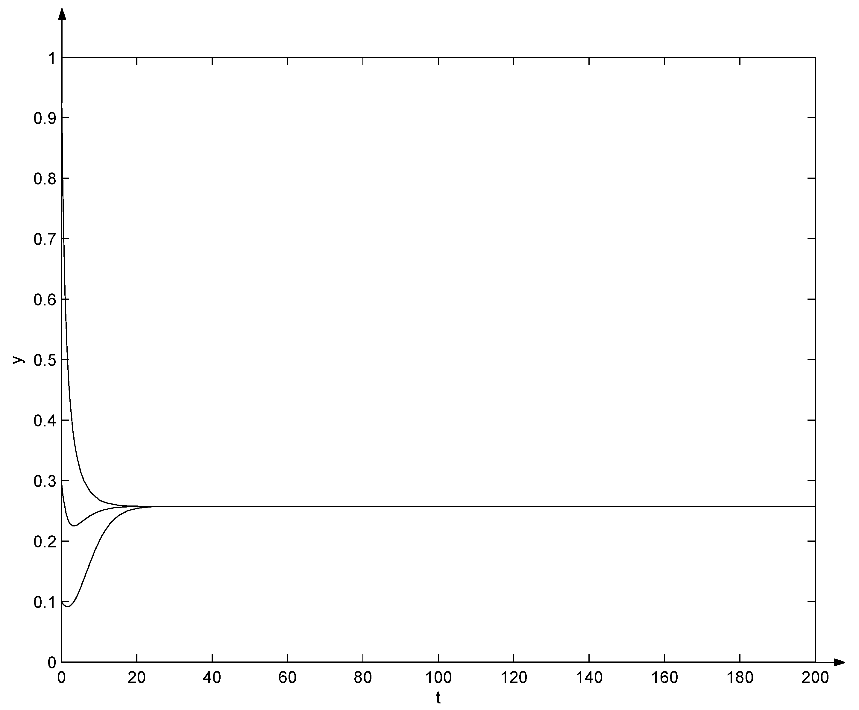
Example 2 

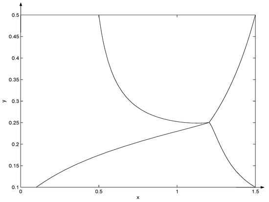
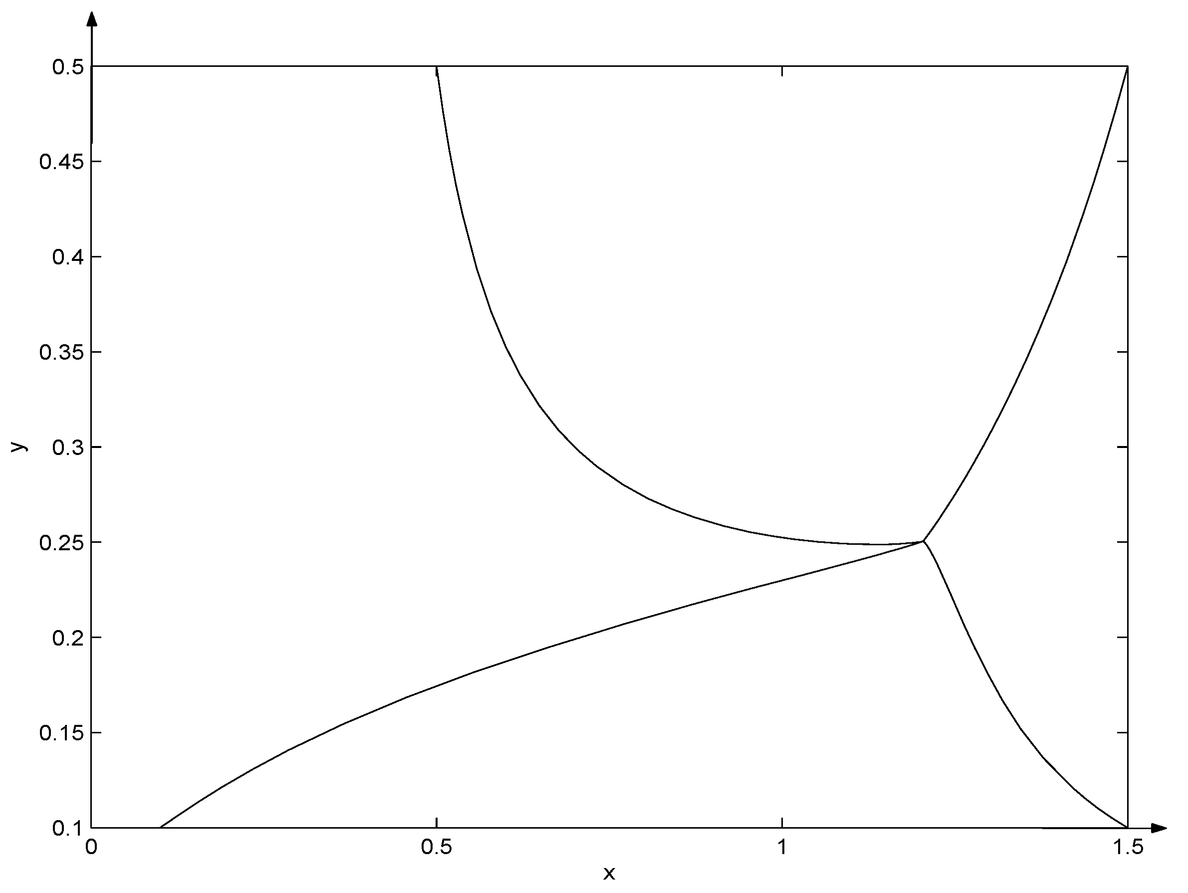
(Example 1 continued). For system (14), the positive equilibrium $(1.2040,0.2505)$ is globally asymptotically stable, which can be seen from Figure 1. Note that in Figure 1, four trajectories start from initial points $(0.5,0.5)$, $(0.1,0.1)$, $(1.5,0.1)$, and $(1.5,0.5)$, respectively, and all converge $(1.2040,0.2505)$ as t tends to $+\infty$.

Figure 1. Four trajectories for system (14) when $\tau =0$.

Remark 3. 

Generally speaking, the exploited population should be mature population, which is more in line with the economic and biological views of renewable resource management. If

$$(a-E_1)\left[f-(d+E_2)m_2\right]>b{m}_1(d+E_2),x^{*}>\frac{a-E_1}{2b},c{m}_2\le f{m}_3,$$

then the positive equilibrium $(x^{*},y^{*})$ of system (7) is globally asymptotically stable for $\tau =0$. From the perspective of eco-managers, in order to plan harvest strategies and maintain the sustainable development of the ecosystem, a positive equilibrium that is asymptotically stable may be required [28].

4.2. Global Asymptotic Stability of Positive Equilibrium for $\tau \ne 0$

In this subsection, we will study the global asymptotical stability of positive equilibrium $(x^{*},y^{*})$ for system (7) by constructing Lyapunov function.

Let $x\left(t\right)=x^{*}+u\left(t\right),y\left(t\right)=y^{*}+v\left(t\right)$, linearized system of system (7) is

$$\left\{\begin{array}{c}{u}^{\prime }=A_{1}u\left(t\right)-A_{2}v\left(t\right),\hfill \\ v^{\prime }=A_{3}u(t-\tau )-A_{4}v\left(t\right)+A_{5}v(t-\tau ),\hfill \end{array}\right.$$

(28)

where

$$\left\{\begin{array}{c}{A}_1=a-2b{x}^{*}-\frac{c{y}^{*}(m_1+m_3{y}^{*})}{{(m_1+m_2{x}^{*}+m_3{y}^{*})}^2}-E_1,A_2=\frac{c{x}^{*}(m_1+m_2{x}^{*})}{{(m_1+m_2{x}^{*}+m_3{y}^{*})}^2},\hfill \\ A_3=\frac{f{e}^{-d_i\tau }{y}^{*}(m_1+m_3{y}^{*})}{{(m_1+m_2{x}^{*}+m_3{y}^{*})}^2},A_4=d+2p{y}^{*}+E_2,A_5=\frac{f{e}^{-d_i\tau }{x}^{*}(m_1+m_2{x}^{*})}{{(m_1+m_2{x}^{*}+m_3{y}^{*})}^2}.\hfill \end{array}\right.$$

(29)

Rewrite the system (28) as follows:

$$\left\{\begin{array}{c}{u}^{\prime }=A_{1}u\left(t\right)-A_{2}v\left(t\right),\hfill \\ v^{\prime }=A_{3}u\left(t\right)+(A_5-A_4)v\left(t\right)-A_3{\int }_{t-\tau }^t{u}^{\prime }\left(s\right)ds-A_5{\int }_{t-\tau }^t{v}^{\prime }\left(s\right)ds.\hfill \end{array}\right.$$

(30)

In the following, we will construct a positive definite Lyapunov function $V\left(t\right)$ and prove that $V^{\prime }\left(t\right)<0$. Thus, if the global asymptotic stability of origin equilibrium $(0,0)$ for system (30) is obtained, we can have the global asymptotic stability of positive equilibrium $(x^{*},y^{*})$ for system (7).

First, let $V_{11}\left(t\right)=v^2\left(t\right)$, then

$$V_{11}^{\prime }\left(t\right)=2v\left(t\right)\left[A_{3}u\left(t\right)+(A_5-A_4)v\left(t\right)-A_3{\int }_{t-\tau }^t{u}^{\prime }\left(s\right)ds-A_5{\int }_{t-\tau }^t{v}^{\prime }\left(s\right)ds\right]$$

$$=2A_{3}u\left(t\right)v\left(t\right)+2(A_5-A_4)v^2\left(t\right)-A_3{\int }_{t-\tau }^t\left[2A_{1}u\left(s\right)v\left(t\right)-2A_{2}v\left(s\right)v\left(t\right)\right]ds$$

$$-A_5{\int }_{t-\tau }^t\left[2A_{3}u(s-\tau )v\left(t\right)-2A_{4}v\left(s\right)v\left(t\right)+2A_{5}v\left(t\right)v(s-\tau )\right]ds.$$

By the inequality $2ab\le a^2+b^2$, we have

$$V_{11}^{\prime }\left(t\right)\le A_3(u^2\left(t\right)+v^2\left(t\right))+(A_2{A}_3+A_4{A}_5+|A_1|A_3+A_3{A}_5+A_5^2)v^2\left(t\right)\tau$$

$$+2(A_5-A_4)v^2\left(t\right)+(A_2{A}_3+A_4{A}_5){\int }_{t-\tau }^t{v}^2\left(s\right)ds+\left|A_1\right|A_3{\int }_{t-\tau }^t{u}^2\left(s\right)ds$$

$$+A_3{A}_5{\int }_{t-\tau }^t{u}^2(s-\tau )ds+A_5^2{\int }_{t-\tau }^t{v}^2(s-\tau )ds.$$

Second, let

$$V_{12}\left(t\right)=(A_2{A}_3+A_4{A}_5){\int }_{t-\tau }^t{\int }_z^t{v}^2\left(s\right)dsdz+\left|A_1\right|A_3{\int }_{t-\tau }^t{\int }_z^t{u}^2\left(s\right)dsdz$$

$$+A_3{A}_5{\int }_{t-\tau }^t{\int }_z^t{u}^2(s-\tau )dsdz+A_5^2{\int }_{t-\tau }^t{\int }_z^t{v}^2(s-\tau )dsdz,$$

then

$$V_{12}^{\prime }\left(t\right)=(A_2{A}_3+A_4{A}_5)\left[\tau v^2\left(t\right)-{\int }_{t-\tau }^t{v}^2\left(s\right)ds\right]+\left|A_1\right|A_3\left[\tau u^2\left(t\right)-{\int }_{t-\tau }^t{u}^2\left(s\right)ds\right]$$

$$+A_3{A}_5\left[\tau u^2(t-\tau )-{\int }_{t-\tau }^t{u}^2(s-\tau )ds\right]+A_5^2\left[\tau u^2(t-\tau )-{\int }_{t-\tau }^t{u}^2(s-\tau )ds\right].$$

Therefore,

$$V_{11}^{\prime }\left(t\right)+V_{12}^{\prime }\left(t\right)\le 2A_{3}u\left(t\right)v\left(t\right)+(2A_2{A}_3+2A_4{A}_5+A_5^2+|A_1|A_3+A_3{A}_5)\tau v^2\left(t\right)$$

$$+2(A_5-A_4)v^2\left(t\right)+\left|A_1\right|A_3\tau u^2\left(t\right)+A_5^2\tau v^2(t-\tau )+A_3{A}_5\tau u^2(t-\tau ).$$

Third, let

$$V_{13}\left(t\right)=A_5^2\tau {\int }_{t-\tau }^t{v}^2\left(s\right)ds+A_3{A}_5\tau {\int }_{t-\tau }^t{u}^2\left(s\right)ds,$$

then

$$V_{13}^{\prime }\left(t\right)=A_5^2\tau [v^2\left(t\right)-v^2(t-\tau )]+A_3{A}_5\tau [u^2\left(t\right)-u^2(t-\tau )].$$

If $V_1\left(t\right)=V_{11}\left(t\right)+V_{12}\left(t\right)+V_{13}\left(t\right)$, we have

$$V_1^{\prime }\left(t\right)\le v^2\left(t\right)\left[2(A_5-A_4)+(2A_2{A}_3+2A_4{A}_5+A_5^2+|A_1|A_3+A_3{A}_5)\tau \right]$$

$$+u^2\left(t\right)\tau \left(\right|A_1|A_3+A_3{A}_5)+2A_{3}u\left(t\right)v\left(t\right).$$

Assume $V_2\left(t\right)=u^2\left(t\right)$, then

$$V_2^{\prime }\left(t\right)=2A_1{u}^2\left(t\right)-2A_{2}u\left(t\right)v\left(t\right).$$

Last, let $V\left(t\right)=V_1\left(t\right)+V_2\left(t\right)$, therefore,

$$V^{\prime }\left(t\right)\le v^2\left(t\right)\left[2(A_5-A_4)+(2A_2{A}_3+2A_4{A}_5+A_5^2+|A_1|A_3+A_3{A}_5)\tau \right]$$

$$+2(A_3-A_2)u\left(t\right)v\left(t\right)+u^2\left(t\right)\left[\right(2A_1+\left(\right|A_1|A_3+A_3{A}_5\left)\tau \right]$$

$$\le v^2\left(t\right)\left[2(A_5-A_4)+|A_3-A_2|+(2A_2{A}_3+2A_4{A}_5+A_5^2+|A_1|A_3+A_3{A}_5)\tau \right]$$

$$+u^2\left(t\right)\left[\right(2A_1+|A_3-A_2|+(|A_1|A_3+A_3{A}_5\left)\tau \right].$$

According to the definition of $A_4$ and $A_5$, we have $A_4>A_5$. Obviously, if

$$\left\{\begin{array}{c}|A_3-A_2|<min\left\{-2A_1,2(A_4-A_5)\right\},A_1<0\hfill \\ \tau <min\left\{\frac{2(A_4-A_5)-|A_3-A_2|}{2A_2{A}_3+2A_4{A}_5+2A_5^2+\left|A_1\right|A_3+A_3{A}_5},\frac{-2A_1-|A_3-A_2|}{|A_1|A_3+A_3{A}_5}\right\}\hfill \end{array}\right.$$

(31)

holds, then $V^{\prime }\left(t\right)<0$. Through the above analysis, $V\left(t\right)$ is a positive definite function and $V^{\prime }\left(t\right)$ is negative definite when the conditions (10) and (31) hold. Thus, $(0,0)$ of the system (30) is globally asymptotically stable. That is, the positive equilibrium $(x^{*},y^{*})$ for system (7) is globally asymptotically stable. We can get the following theorem.

Theorem 6. 

If the conditions (10) and (31) hold, the positive equilibrium $(x^{*},y^{*})$ of system (7) is globally asymptotically stable for $\tau \ne 0$.

Remark 4. 

From the condition (31), we obtain the interval $[0,{\tau }^{**})$, where

$${\tau }^{**}=min\left\{\frac{2(A_4-A_5)-|A_3-A_2|}{2A_2{A}_3+2A_4{A}_5+2A_5^2+\left|A_1\right|A_3+A_3{A}_5},\frac{-2A_1-|A_3-A_2|}{|A_1|A_3+A_3{A}_5}\right\};$$

from the condition (10) and Remark 2, we have the interval $[0,{\tau }^{*})$. Therefore, when $\tau <min\{{\tau }^{*},{\tau }^{**}\}$, Theorem 6 holds. This implies that the value of time delay determines the global asymptotic stability of the positive equilibrium.

Example 3. 

Let $a=1$, $b=0.6$, $c=0.15$, $d=0.02$, $p=0.9$, $f=0.1$, $m_1=0.1$, $m_2=0.2$, $m_3=0.3$, $E_1=0.1$, $E_2=0.05$, $d_i=0.01$, and $\tau =0.2$, the system (7) becomes

$$\left\{\begin{array}{c}{x}^{\prime }\left(t\right)=x\left(1-0.6x-\frac{0.15y}{0.1+0.2x+0.3y}\right)-0.1x,\hfill \\ y^{\prime }\left(t\right)=-0.02y-0.9y^2+\frac{0.1e^{-0.002}x(t-0.2)y(t-0.2)}{0.1+0.2x(t-0.2)+0.3y(t-0.2)}-0.05y.\hfill \end{array}\right.$$

(32)

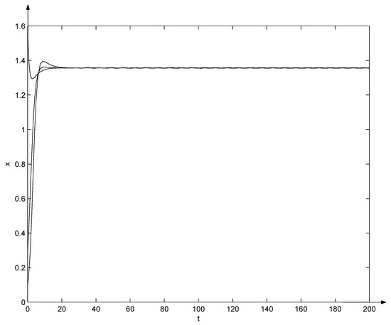
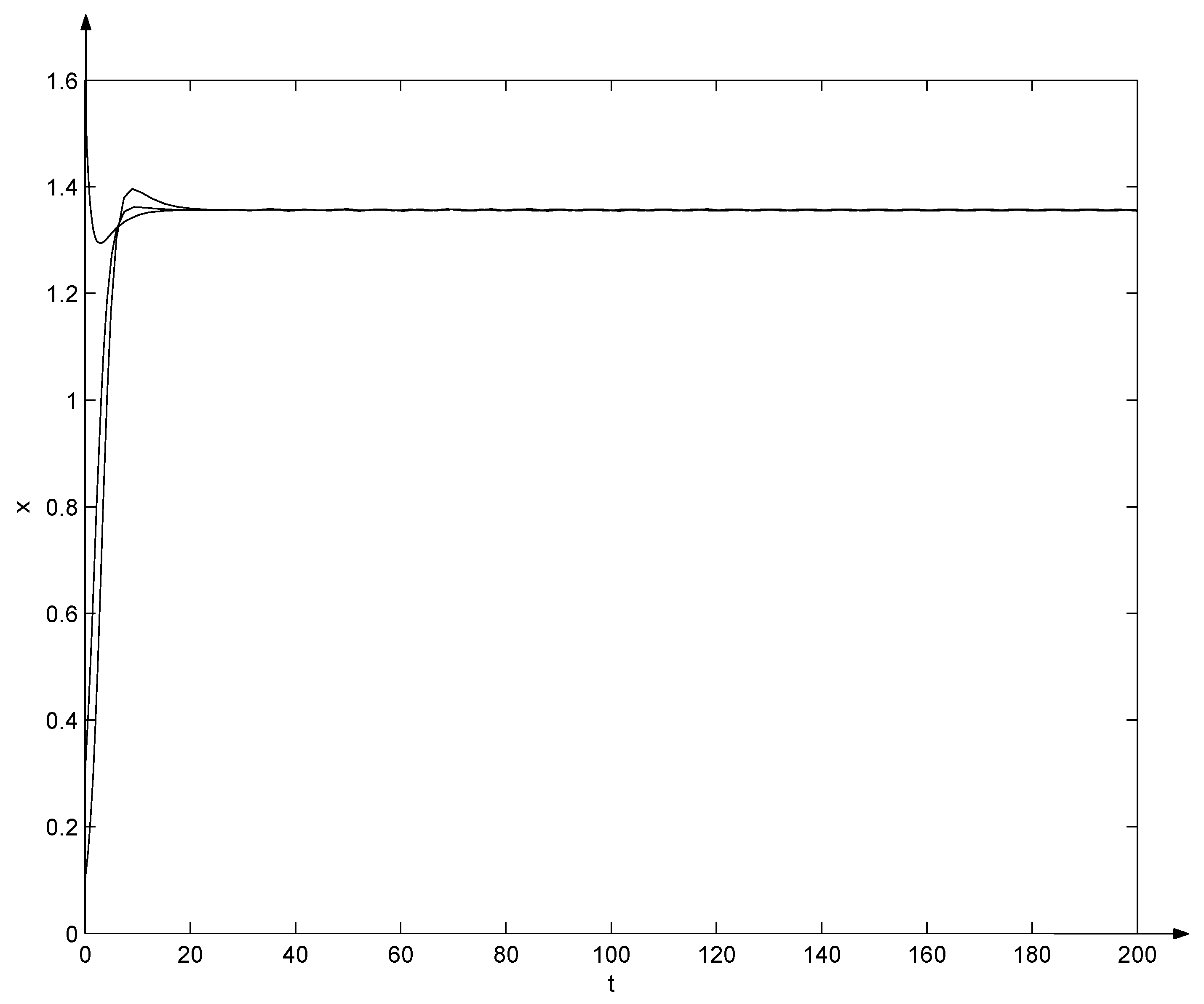
Clearly, $(a-E_1)(f{e}^{-d_i\tau }-(d+E_2)m_2)-b(d+E_2)m_1=0.073$ and from the Equation (29), $A_1=-0.7618$, $A_2=0.3755$, $A_3=0.023$, $A_4=0.5337$, $A_5=0.2498$, $-2A_1=1.5237,A_3-A_2=-0.3528$, $2(A_4-A_5)=0.5678$, $\frac{-2A_1-|A_3-A_2|}{|A_1|A_3+A_3{A}_5}=51.1008$, $\frac{2(A_4-A_5)-|A_3-A_2|}{2A_2{A}_3+2A_4{A}_5+2A_5^2+\left|A_1\right|A_3+A_3{A}_5}=0.4983$. That is, conditions (10) and (31) hold. Due to Theorem 6, the positive equilibrium $(1.3565,0.2576)$ of system (32) is globally asymptotically stable, which can also be seen from Figure 2 and Figure 3. Note that in Figure 2 and Figure 3, three trajectories start from initial points $(1.6,1.0)$, $(0.1,0.1)$, and $(0.3,0.3)$, respectively, and all converge $(1.3565,0.2576)$ as t tends to $+\infty$.

Figure 2. Evolutions $x\left(t\right)$ of system (32).

Figure 3. Evolutions $y\left(t\right)$ of system (32).

5. Conclusions

In this paper, we investigate dynamics of a stage-structured density-dependent predator–prey system with Beddington–DeAngelis functional response and harvesting.

First, according to the sign for real part of eigenvalue, the local stability of the origin equilibrium $(0,0)$ and the boundary equilibrium $\left(\frac{a-E_1}{b},0\right)$ is determined.

In addition, we discuss local stability of positive equilibrium $(x^{*},y^{*})$ for the case of $\tau =0$ and $\tau \ne 0$, respectively. When $\tau =0$, the positive equilibrium $(x^{*},y^{*})$ of system (7) is locally asymptotically stable. However, when $\tau \ne 0$, the local stability of positive equilibrium $(x^{*},y^{*})$ of the system (7) includes the following three cases:

(i) If (10), (13), and (18) hold, the positive equilibrium $(x^{*},y^{*})$ of system (7) is locally asymptotically stable for any $\tau \ge 0$;

(ii) If (10) and (19) hold, when $\tau$ increases and passes ${\tau }_0$, the stability of positive equilibrium $(x^{*},y^{*})$ for system (7) switches from local asymptotical stability to unstability and bifurcates into two periodic solutions with small amplitudes;

(iii) If (10) and (21) hold, there is a positive integer k such that the positive equilibrium $(x^{*},y^{*})$ of system (7) has k switches from stability to instability to stability, which shows when the delay $\tau$ passes the critical value ${\tau }_j^{+},j=0,1,2,\dots ,k-1$, the positive equilibrium $(x^{*},y^{*})$ of system (7) loses its stability and Hopf bifurcation occurs.

Last, we consider the global asymptotical stability of the positive equilibrium $(x^{*},y^{*})$ for system (7). When $\tau =0$, stability theory of the periodic solution is used to prove that the positive equilibrium $(x^{*},y^{*})$ is globally asymptotically stable by contradiction; when $\tau \ne 0$, by constructing Lyapunov functions we prove the positive equilibrium $(x^{*},y^{*})$ for system (7) is globally asymptotically stable. Moreover, examples are given to illustrate the obtained results.

The predator–prey model studied in this paper, where not only the prey density dependence but also the predator density dependence are considered such that the system conforms to real biological environment. In Remarks 1, 2, and 4, we explain the effect of time delay on the stability of boundary equilibrium, the existence of the positive equilibrium, and the global asymptotic stability of the positive equilibrium, respectively. Moreover, we study the effect of harvesting on the global asymptotic stability of the positive equilibrium in Remark 3. Simultaneously, regarding the predator density-dependent mortality rate p, by Theorem 1 and the condition 10, the parameter p does not affect the stability of boundary equilibrium, the existence of the positive equilibrium, respectively. As $x^{*},y^{*},a_i(i=1,2,\cdots ,4),A_j(j=1,2,\cdots ,5)$ all contain parameter p, the predator density-dependent mortality rate p not only affects the local asymptotic stability of the positive equilibrium by Theorems 2 and 4, but also the global asymptotic stability of the positive equilibrium by Theorems 5 and 6. However, we cannot describe exactly how the predator density-dependent mortality rate affects the stability of the positive equilibrium. In our future work, we will further study the influence of parameter p on the predator–prey system.

References

- Fatma, B.; Ali, Y.; Chandan, M. Effects of fear in a fractional-order predator-prey system with predator density-dependent prey mortality. Chaos Soliton. Fract. 2021, 145, 110711. [Google Scholar]
- Jiang, X.; Chen, X.; Huang, T.; Yan, H. Bifurcation and Control for a Predator-Prey System With Two Delays. IEEE Trans. Circuits Syst. II 2021, 68, 376–380. [Google Scholar] [CrossRef]
- Liu, J.; Hu, J.; Yuen, P. Extinction and permanence of the predator-prey system with general functional response and impulsive control. Appl. Math. Model. 2020, 88, 55–67. [Google Scholar] [CrossRef]
- Qiu, H.; Guo, S.; Li, S. Stability and Bifurcation in a Predator–Prey System with Prey-Taxis. Int. J. Bifurcat. Chaos 2020, 30, 2050022. [Google Scholar] [CrossRef]
- Molla, H.; Sarwardi, S.; Sajid, M. Predator-prey dynamics with Allee effect on predator species subject to intra-specific competition and nonlinear prey refuge. J. Math. Comput. Sci. 2021, 25, 150–165. [Google Scholar]
- Roy, J.; Barman, D.; Alam, S. Role of fear in a predator-prey system with ratio-dependent functional response in deterministic and stochastic environment. Biosystems 2020, 197, 104176. [Google Scholar] [CrossRef]
- Song, D.; Li, C.; Song, Y. Stability and cross-diffusion-driven instability in a diffusive predator–prey system with hunting cooperation functional response. Nonlinear Anal. Real 2020, 54, 103106. [Google Scholar] [CrossRef]
- Köhnke, M.C.; Siekmann, I.; Seno, H.; Malchow, H. A type IV functional response with different shapes in a predator–prey model. J. Theor. Biol. 2020, 505, 110419. [Google Scholar] [CrossRef] [PubMed]
- Li, H.; Takeuchi, Y. Dynamics of the density dependent predator-prey system with Beddington-DeAngelis functional response. J. Math. Anal. Appl. 2011, 374, 644–654. [Google Scholar] [CrossRef] [Green Version]
- May, R.M. Stability and Complexity in Model Ecosystems (Monographs in Population Biology); Princeton University Press: Princeton, NJ, USA, 1973; Volume 6. [Google Scholar]
- Oaten, A.; Murdoch, W.W. Functional response and stability in predator–prey systems. Am. Nat. 1975, 109, 289–298. [Google Scholar] [CrossRef]
- Vos, M.; Moreno Berrocal, S.; Karamaouna, F.; Hemerik, L.; Vet, L.E.M. Plant-mediated indirect effects and the persistence of parasitoid—Herbivore communities. Ecol. Lett. 2001, 4, 38–45. [Google Scholar] [CrossRef]
- Gross, T.; Ebenhöh, W.; Feudel, U. Enrichment and food chain stability: The impact of different forms of predator–prey interactions. J. Theor. Biol. 2004, 227, 349–358. [Google Scholar] [CrossRef] [PubMed] [Green Version]
- McCann, K.; Rasmussen, J.; Umbanhowar, J. The dynamics of spatially coupled food webs. Ecol. Lett. 2005, 8, 513–523. [Google Scholar] [CrossRef] [PubMed]
- Beddington, J.R. Mutual interference between parasites or predators and its effect on searching efficiency. J. Anim. Ecol. 1975, 44, 331–340. [Google Scholar] [CrossRef] [Green Version]
- DeAngelis, D.L.; Goldstein, R.A.; O’Neil, R.V. A model of trophic interaction. Ecology 1975, 56, 881–892. [Google Scholar] [CrossRef]
- Holling, C.S. The components of predation as revealed by a study of small-mammal predation of the European pine sawfly. Canad. Entomol. 1959, 91, 293–320. [Google Scholar] [CrossRef]
- Holling, C.S. Some characteristics of simple types of predation and parasitism. Can. Entomol. 1959, 91, 385–395. [Google Scholar] [CrossRef]
- Solomon, M.E. The natural control of animal populations. J. Anim. Ecol. 1949, 18, 1–35. [Google Scholar] [CrossRef]
- Holling, C.S. The functional response of invertebrate predators to prey density. Mem. Entomol. Soc. Can. 1966, 48, 1–87. [Google Scholar] [CrossRef]
- Kratina, P.; Vos, M.; Bateman, A.; Anholt, B.R. Functional response modified by predator density. Oecologia 2009, 159, 425–433. [Google Scholar] [CrossRef]
- Aiello, W.G.; Freedman, H.I. A time-delay model of single-species growth with stage structure. Math. Biosci. 1990, 101, 139–153. [Google Scholar] [CrossRef]
- Freedman, H.I.; Wu, J.H. Persistence and global asymptotic stability of single species dispersal models with stage structure. Quart. Appl. Math. 1991, 2, 351–371. [Google Scholar] [CrossRef] [Green Version]
- Zhao, X.; Zeng, Z. Stationary distribution and extinction of a stochastic ratio-dependent predator–prey system with stage structure for the predator. Physica A 2020, 545, 123310. [Google Scholar] [CrossRef]
- Hu, D.; Li, Y.; Liu, M.; Bai, Y. Stability and Hopf bifurcation for a delayed predator–prey model with stage structure for prey and Ivlev-type functional response. Nonlinear Dyn. 2020, 99, 3323–3350. [Google Scholar] [CrossRef]
- Ghosh, B.; Zhdanova, O.L.; Barman, B.; Frisman, E.Y. Dynamics of stage-structure predator-prey systems under density-dependent effect and mortality. Ecol. Complex. 2020, 41, 100812. [Google Scholar] [CrossRef]
- Liu, S.; Beretta, E. A stage-structured predator-prey model of Beddington-DeAngelis type. SIAM J. Appl. Math. 2006, 66, 1101–1129. [Google Scholar] [CrossRef]
- Song, X.; Chen, L. Optimal harvesting and stability for a two species competitive system with stage structure. Math. Biosci. 2001, 170, 173–186. [Google Scholar] [CrossRef]
- She, Z.; Li, H. Dynamics of a density-dependent stage-structured predator–prey system with Beddington–DeAngelis functional response. J. Math. Anal. Appl. 2013, 406, 188–202. [Google Scholar] [CrossRef]
- Qu, Y.; Wei, J. Bifurcation analysis in a predator-prey system with stage-structure and harvesting. J. Franklin. Inst. 2010, 347, 1097–1113. [Google Scholar] [CrossRef]
- Xiao, D.; Jennings, L.S. Bifurcations of a ratio-dependent predator–prey system with constant rate harvesting. SIAM J. Appl. Math. 2005, 65, 737–753. [Google Scholar] [CrossRef]
- Chen, J.; Huang, J.; Ruan, S.; Wang, J. Bifurcations of invariant tori in predator–prey models with seasonal prey harvesting. SIAM J. Appl. Math. 2013, 73, 1876–1905. [Google Scholar] [CrossRef]
- Yan, X.; Zhang, C. Global stability of a delayed diffusive predator–prey model with prey harvesting of Michaelis–Menten type. Appl. Math. Lett. 2021, 114, 106904. [Google Scholar] [CrossRef]
- Mortuja, M.G.; Chaube, M.K.; Kumar, S. Dynamic analysis of a predator-prey system with nonlinear prey harvesting and square root functional response. Chaos Soliton. Fract. 2021, 148, 111071. [Google Scholar] [CrossRef]
- Brauer, F.; Soudack, A. Stability regions in predator-prey systems with constant rate prey harvesting. J. Math. Biol. 1979, 8, 55–71. [Google Scholar] [CrossRef]
- May, R.M.; Beddington, J.R.; Clark, C.W.; Holt, S.J.; Laws, R.M. Management of multispecies fisheries. Science 1979, 205, 267–277. [Google Scholar] [CrossRef]
- Hale, J.K. Theory of Functial Differential Equations; Springer: New York, NY, USA, 1977. [Google Scholar]
- Kar, T.K.; Pahari, U.K. Modelling and analysis of a prey-predator system with stage-structure and harvesting. Nonlinear Anal. 2007, 8, 601–609. [Google Scholar] [CrossRef]
- Hale, J. Ordinary Differential Equation; Krieger Publishing: Malabar, FL, USA, 1980. [Google Scholar]
Publisher’s Note: MDPI stays neutral with regard to jurisdictional claims in published maps and institutional affiliations. |
© 2021 by the authors. Licensee MDPI, Basel, Switzerland. This article is an open access article distributed under the terms and conditions of the Creative Commons Attribution (CC BY) license (https://creativecommons.org/licenses/by/4.0/).