Detection of Cadmium and Lead Heavy Metals in Soil Samples by Portable Laser-Induced Breakdown Spectroscopy

Abstract

Heavy metal pollution in soil is becoming more and more serious. LIBS is one of the most promising technologies for rapid detection of heavy metal contamination in soil. However, due to the wide variety of soils and complex matrices, accurate quantification remains a challenge. In total, 451 soil samples were prepared and detected by the portable detector of LIBS, which were divided into six categories based on the compactness of the soil pellets, and a separate quantitative model for each type of soil sample was used for quantitative analysis by external standard method. It did not need a lot of data to train the model, and only a small number of calibration samples could be used for quantitative analysis of a large number of samples. The results showed that 78 standard samples and 334 collected samples were quantitatively analyzed by 39 standard samples. Compared with the standard value, the correlation coefficients were all above 0.95. A comparative experiment indicated that the portable LIBS system combined with soil classification and calibration methods can achieve fast and accurate quantitative detection.

1. Introduction

Heavy metal pollution in soil, mainly caused by industrial production, automobile exhaust and household garbage, has become increasingly problematic. Cadmium (Cd), chromium (Cr), copper (Cu), nickel (Ni), lead (Pb) and zinc (Zn) in the air, water and soil enter into plants through adsorption and absorption. Heavy metals are harmful to the environment and the human body. For example, Pb and its compounds enter the human body mainly through the respiratory tract and the digestive tract. Pb can harm human health through atmosphere, drinking water and food. In the human body, Pb is mainly deposited in the bones in the form of insoluble lead phosphate, and a small amount is also accumulated in the brain, liver, kidney, and other organs. The rapid development of lead smelting industry has also caused more and more wastewater containing Pb to be discharged into ecosystems, especially farmland. As a result, the quality of major food crops is reduced, such as rice and vegetables, which in turn reduces production and cause human diseases. At present, the main techniques for detecting heavy metals in soil are the traditional laboratory analysis methods, such as flame atomic absorption spectrometry (FAAS) [1], atomic fluorescence spectroscopy (AFS) [2], inductively coupled plasma-mass spectroscopy (ICP-MS) [3,4], etc. The detection results of these methods are accurate and reliable, but they are time-consuming and require cumbersome sample preparation, which cannot meet the demands of real-time on-site detection and undergo green analysis.

Laser-induced breakdown spectroscopy (LIBS) is a widely used technique for elemental analysis which is based on atomic emission spectroscopy [5]. This method has the advantages of in situ, simultaneous analysis of multiple elements and fast detection speed, and it has been proven to be an effective soil element analysis method [6,7,8,9]. Because the form of the sample is totally unrestricted, LIBS is greatly affected by the sample matrix effect, especially for solid samples. Researchers still must strive to improve the stability, the sensitivity and accuracy of the measurement results [10,11,12]. For soil samples, which are compound samples with complex matrices, several inherent drawbacks, such as mutual interference of elements, low concentration of heavy metals, poor repeatability, shorter plasma lifetime, restrict the use of LIBS [13,14]. Khalil et al. used the double-pulse LIBS technique to enhance the soil LIBS signal intensity. The two lasers were collinear with the wavelengths of 1064 and 266 nm. The results showed that the minimum detection concentrations of Cr and Pb were as low as 6.7 mg·kg⁻¹ and 5.1 mg·kg⁻¹ [15]. Ge et al. developed a device using atmospheric pressure glow discharge as the second excitation source coupled with laser ablation for direct analyzing of soil samples. The respective linear correlation coefficients (R²) were 0.9953, 0.9897, and 0.9961. Moreover, the limits of detection (LOD) of Zn, Pb, and Cd were 0.68, 2.71, and 0.31 mg·kg⁻¹, respectively [16]. Umar et al. implied the LIBS technique with sample heating to detect Pb in soil. The emission line intensities were enhanced and the limit of detection of lead was 3.8 mg·kg⁻¹ [17]. Marcella et al. used LIBS to detect potentially toxic metals in contaminated soil and found an R² value of 0.974 for Cr, which was better than that achieved by inductively coupled plasma optical emission spectrometry and atomic absorption spectroscopy [18]. All of the above research works proved that LIBS technology can be used for detection of heavy metal pollution in soil. However, for different types of soil samples, the detection accuracy needs to be improved.

Recently, the precision and accuracy of LIBS quantitative analysis have improved with the use of the chemometric methods, which can eliminate the interference factors and extract useful information from the LIBS spectrum. Single-pulse and double-pulse LIBS coupled with partial least squares regression (PLSR) and a least square support vector regression (LS-SVR) quantitative model were employed to analyze nutrient elements in soil samples. For all nutrient elements, the correlation coefficient R2 was greater than 0.95 in both the calibration and prediction sets [19]. The LIBS technique coupled with partial least squares (PLS) were used to quantify Ca in soil, and the root mean square error of cross-validation (RMSECV) was 0.314 wt.%, and the R2 can achieved a value of 0.99 [20]. The handheld LIBS combined with multivariate regression methods were used to detect nutrient elements in soil. The regression methods used included PLSR, least absolute shrinkage and selection operator regression (Lasso), and Gaussian process regression (GPR). The best prediction results were obtained for Ca, K, Mg and Fe [21]. LIBS and single/multivariate regression were used to quantify the main components in soil, and the R² values of Cr for the PLSR and SVR calibrations were 0.98 and 0.99, respectively [22]. The regression methods of PLSR and LS-SVR were used to quantitatively analyze the heavy metal element Cd in soil with the LIBS technique [23]. Under argon atmosphere, the LS-SVR model obtained the best performance, which demonstrated the ability of LIBS to perform accurate quantitative detection of Cd in soil. It was demonstrated that the signals for soil samples are strongly affected by the matrix effects and that classification of data is necessary as a preliminary step of quantitative analysis. Principal component analysis (PCA) was considered to be a very effective method of data classification, but it also has limitations in the highly variable physical and chemical parameters of soil samples [24]. Usually, the soil samples are prepared as pellets to be tested using LIBS. The compactness of the pellets has great influence on the ablative pit and directly affects the intensity of the spectral. At present, research on soil classification is mainly based on machine learning algorithms; there is little research about classification according to the physical and chemical properties of soils which are closely related to soil excitation efficiency.

In this paper, soils were classified according to the compactness of the soil pellets, and then a separate calibration curve was established for each type of soil for quantitative analysis based on the external standard method. Compared with machine learning algorithms, the external standard method had the advantage of requiring less calibration samples. Approximately ten calibration samples can be used for quantitative analysis of a large number of samples. The contents of Cd and Pb in 451 soil samples are studied using the external standard method after classification.

2. Materials and Methods

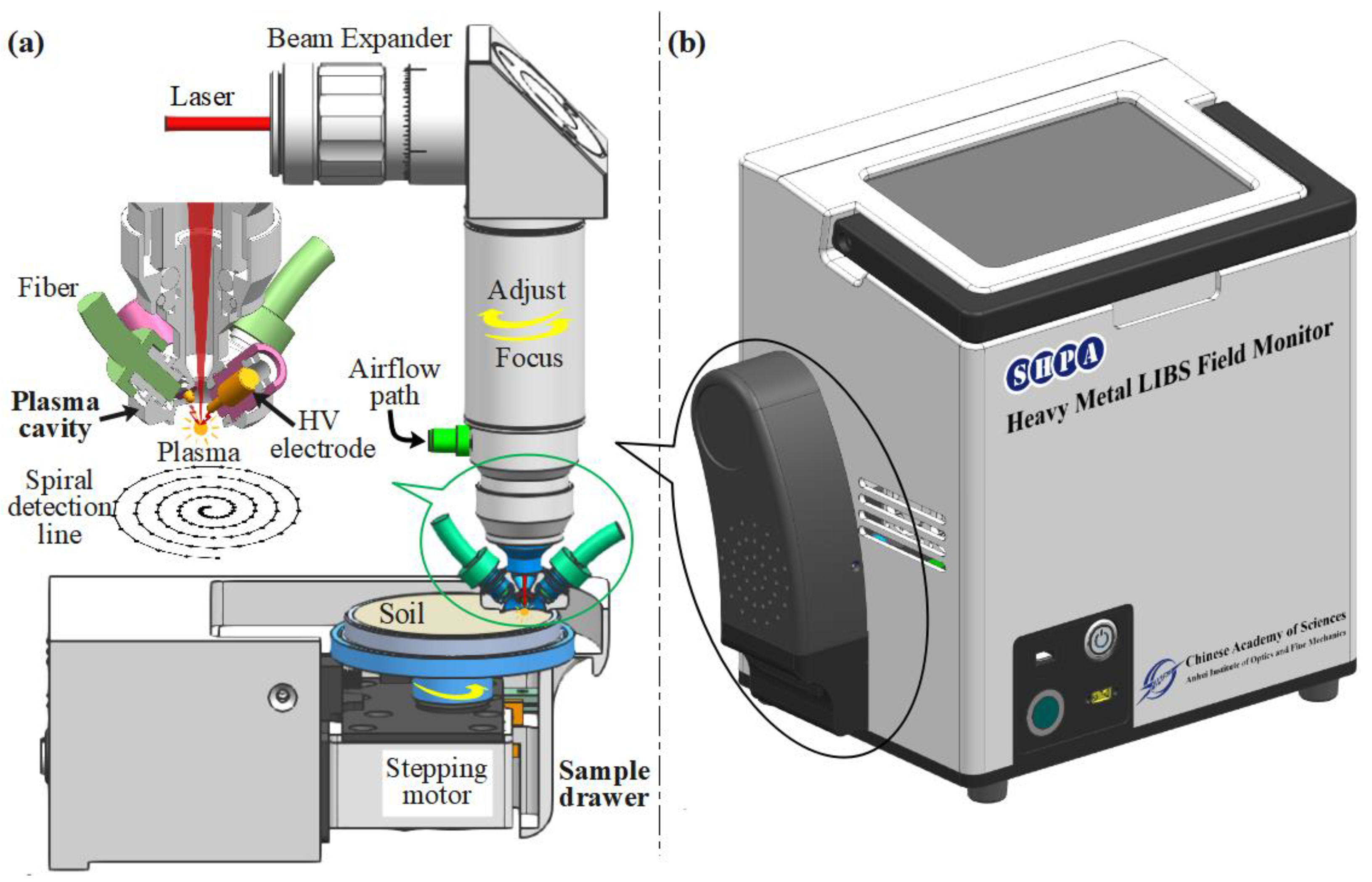
2.1. Experimental Setup

The structure diagram of the portable on-site soil heavy metal laser-induced breakdown spectrum detector is shown in Figure 1. It was independently developed by the research group. Figure 1a illustrates the core structure of spectral signal detection and sample control, which included a spectrum acquisition unit and a sample control unit. The spectral acquisition unit consisted of a laser beam expander, a plasma confinement cavity, spark discharge, and a spectral signal acquisition fiber. The sample control unit was composed of a sample tray, a stepper motor, a screw motor, etc. The laser beam was expanded by a 2.5× beam expander, and then, through a fused silica lens with a focal length of 75 mm, the focus was located outside the hemispherical space constraint cavity, 1.5 mm away from the bottom surface of the constraint cavity. The theoretical focal spot radius was 22.5 µm. The diameter of the hemispherical cavity was 9.6 mm. The laser-induced plasma was enhanced by re-discharge, and the discharge electrode was a tungsten rod with a purity greater than 99.95% and a diameter of 2.5 mm; the distance between the two electrodes was 4 mm, and the discharge parameter was 110 nF and 4.2 kV. The spectral signal was acquired by two bunched fibers (6 × 400 µm) located on the side wall of the hemispherical confinement cavity. The purpose of using two bunched fibers (6 × 400 µm) was to enhance the coupling of plasma optical radiation into the spectrometer. At the same time of spectral acquisition, the air flow was injected through the air valve to discharge the fine dust generated by laser ablation in the hemispherical spatial confinement cavity, which improved the stability of the spectral signal and reduced the degree of contamination of the optical components surface. The parameters of the laser and spectrometer in the portable system are shown in

Table 1. Parameters of the laser and the spectrometer.

Laser (DPS-1064-BS-D)	Wavelength (nm)	1064
	Pulse width (ns)	8
	Divergence (mrad)	1.5
	Repetition rate (Hz)	5
	Pulse energy (mJ)	50
Spectrometer (AVS-MINI-USB2)	Resolution (nm)	0.08~0.12
	Range (nm)	200~450
	Acquisition delay time (µs)	1.25
	Gating time (ms)	1

.

The soil samples were placed on trays controlled by a drawer-like mechanism. The upper surface of the sample was 0.5 mm away from the end face bottom surface of the hemispherical space, a spatially constrained cavity. The sample tray was rotated by a stepper motor, and the stepper motor and the sample tray were transcribed by the screw motor together. Therefore, the trajectory of the laser action point on the surface of the sample was a spiral line during spectral collection, which achieved multi-point non-repetitive controllable spectral signal acquisition, effectively reduced the influence of the non-uniformity of the sample on the detection results, and improved the stability of the spectral data. The sample console was controlled synchronously by the laser’s Q-switched signal.

Laser ablation pits were photographed using commercial microscopes: Nikon ECLIPS Ni-U Vertical microscope (Nikon Eclips Ni-U, Japan).

2.2. Sample Preparation

In the experiment, 60 standard soil samples were purchased (the Henan reference material R & D Center, China). These soils with different matrices were collected from different regions in China. In addition, there were 334 soil samples, including 30 soils collected from a mining area in Tongling, 7 soils from a mining area in Yunnan, and 297 soils collected from Yingshang in Anhui. The contents of Cd and Pb in these soils were detected using ICP-MS. Cd and Pb were added to some of these samples employing a standard addition method. Finally, a total of 452 soil samples with known Cd and Pb concentrations were obtained. The collected soil samples needed to be pre-treated with air-drying, grinding, and sifting. A quantity of 3 g was weighed for each of the samples and pressed into tablets of 30 mm in diameter and 2 mm in thickness under a 10 MPa pressure for 180 s (769YP-40C, KQ, Tianjin, China) [25]. The concentrations of the heavy metals in the 451 soil samples are listed in

Table 2. Statistics of Pb and Cr concentrations in soil samples.

Properties	Cd (mg/kg)	Pb (mg/kg)
Minimum value	0.03	11.30
Maximum value	422.45	1141.13
Mean value	11.77	55.05
Standard deviation values	50.06	89.96

.

A hundred laser-pulsed plasma spectra were collected for each soil sample, with a total of 45,100 LIBS spectra. The acquired spectral data were analyzed using MATLAB software (2021a) and graphed using Origin software (Origin95).

2.3. Influence of Soil Matrix Effects

The main components of the soil are aluminum, silicon, iron, calcium, etc. The content of the main components varied greatly with soil type; for example, the content of aluminum in clay was very high, and clay usually appeared as a very fine powder. However, the content of silicon in the sand was significant, and the sand was characterized by coarse particles and hard texture. The differences in the soil matrix led to differences in the process of interaction between laser and substance, which was reflected in the nonlinear relationship between spectral signal intensity and analyte concentration, and it was difficult to establish a calibration curve, as shown in Figure 2. Matrix effects were a core problem affecting the quantitative analysis of LIBS. One of the ways to solve this problem was to classify the soils in the initial steps of the analysis.

2.4. Classification and Quantitative Analysis Methods

When the soil samples were pressed with the same pressure, the compactness values of different types of soils were very different. For LIBS researchers who are not familiar with soil properties, compactness is the most direct way to distinguish soil types. Moreover, the compactness of the pellets is closely related to the spectral intensity of LIBS. There was almost no dust seen during the laser breakdown on the compact soil pellets, and the ablation pit was very small and very regular. Conversely, when the laser was applied to the surface of the loose soil pellets, a large amount of dust was generated, and the ablation pit was large and irregular. The amount of dust and the size of the ablation pit were determined by the compactness of the pellet when the laser pulse broke down soil pellets. According to the compactness of the pellets, the soil samples were artificially divided into 6 categories.

One soil sample was selected from each of the 6 types of soil samples. The calibration sample was prepared using the standard addition method based on the 6 selected soil samples. The calibration curve was established based on the external standard method to invert the heavy metal content of the other soil samples.

3. Results and Discussion

3.1. Soil Classification and Calibration Model

The two heavy metal elements in soil samples, Cd and Pb, were studied. Observing the spectra of all the soil samples, a characteristic spectral line was selected for each element as the analytical data, such as 228.80 nm for Cd and 405.78 nm for Pb. There was no interfering line around these lines for soil samples. Spectral intensity was obtained by subtracting the baseline from the full spectrum.

Before establishing the quantitative analysis model, all standard samples were classified according to the compactness of the soil pellets, which was not difficult for researchers unfamiliar with edaphology. The results were shown in

Table 3. Soil classification result.

Compactness	Soils
Grade 1	gss7, gss20, gss70, gss71, gss73
Grade 2	gss63, gss67, gss68, gss69, gss76, gss79, gss80, gss81
Grade 3	gss1a, gss54, gss56, gss57, gss62, gss64, gss65, gss66
Grade 4	gss22, gss24, gss32, gss33, gss34, gss36, gss37, gss39, gss40, gss41, gss42, gss43, gss44, gss45, gss46, gss47, gss49, gss59, gss61, gss64, gss72, gss74, gss75, nst2
Grade 5	gss2, gss3a, gss18, gss25, gss38, gss48, gss50, gss52, gss58, gss60, gss77
Grade 6	gsf2, gss17, gss78, gss82

. The compactness of the soil pellets was determined using the ablative pit formed by the laser ablation and the dust generated. Although the classification in this way was subjective, the results prove that there was indeed a close relationship between soil compactness and spectral intensity.

In terms of compactness, soil samples were divided into six grades from loosening to compacted. Grade 1 means that the soil is very compact and rarely produces dust during the laser ablates, and Grade 6 means that the soil pellets are very loose and produce a lot of dust during laser ablation, and that the ablation pits were large and obvious. One soil from each of the six categories was selected for building the quantitative analysis model. They were, respectively, gss71, gss79, gss57, gss72, gss25 and gss82, and the photos of the six grades of soil ablation pits are shown in Figure 3a,b with a corresponding microscope image; magnification was 5.5. According to the observations of the ablation pits, with the exception of gss82, the other five samples had relatively clear edges. The pits of gss71 were small and the outline was clearly visible, and the depth of the pit was about 22 μm. For gss82, it was almost impossible to make out the edge of the ablation pit, and the depth of the pit was about 50 μm. It was also particularly prone to fragmentation during pressing or laser cutting. Soil particles outside the pits were also partially carried away. This microscope was not a very accurate measure of pit depth and was used only for estimation, so it did not measure all pit depths. The diameter of the ablation pit was calculated according to the pixel, and the results were in the following order: 296.85, 313.37, 314.28, 318.91, 399.82, and 467.50 μm. The results were consistent with our previous classification.

Then, a series of standard solutions with different concentrations containing Cd and Pb were configured to establish the calibration curves. The calibration curves are shown in Figure 4. It can be seen that the calibration curves vary greatly from each other among different soil types. The slopes of the Cd calibration curves were, respectively, 2.20, 3.55, 4.26, 5.25, 6.26 and 11.42. The slopes of the Pb calibration curves were, respectively, 0.76, 1.35, 2.19, 2.81, 3.87 and 5.32, and the detailed fitting parameters are shown in

Table 4. Calibration curves of different classes.

Category	Calibration Curve of Cd	R2	Calibration Curve of Pb	R2
1	y = 2.20x + 80.42	0.9823	y = 0.76x + 273.70	0.9610
2	y = 3.55x + 141.41	0.9872	y = 1.35x + 181.72	0.9982
3	y = 4.26x + 140.62	0.9965	y = 1.49x + 208.10	0.9507
4	y = 5.25x + 99.86	0.9954	y = 2.01x + 216.86	0.9836
5	y = 6.26x + 107.40	0.9927	y = 3.85x + 131.42	0.9867
6	y = 11.42x + 104.07	0.9937	y = 5.32x + 40.72	0.9895

. When the concentration of heavy metals was too high, the spectral intensity showed a nonlinear relationship with the concentration, and only the linear fitting part was left in this work. The squares of the linear correlation coefficient R were all greater than 0.98. The looser the soil, the higher the slope of the calibration curve. This may be closely related to the ablation quality. The looser the soil, the larger the ablative pit and the greater the ablative mass, so the corresponding spectral intensity was stronger.

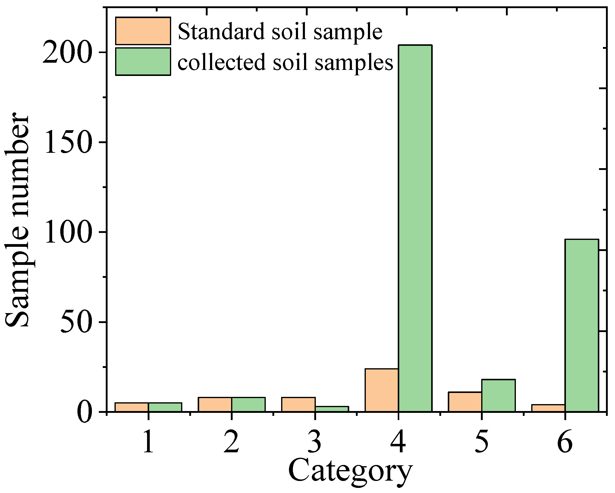
3.2. Classification Results of Soil Samples Collected

There were 334 soil samples collected from Tongling and Yunnan mining areas and Anhui Province in total. When detected by LIBS, we paid attention to the dust situation and the size of the ablative pit, and then each sample was classified into one of the above-mentioned six categories based on the amount of dust produced and the size of the ablation pit. The specific classification results are shown in Figure 5. The largest number of samples was classified in the fourth category, and interestingly, this distribution trend was the same as that of the standard sample.

Only five soil samples were classified as Category 1: one was from the Yunnan mining area, one was from the Tongling mining area, and the other three were from the Anhui Yingshang area. Eight soil samples were classified as Category 2: three from the Yunnan mining area, three from the Tongling mining area and two from the Anhui Yingshang area. Three samples were classified as Category 3, including two from Yunnan Province and one from the Yingshang area. The eighteen samples of Category 5 were mostly from Yingshang of Anhui Province. The number of samples in Categories 4 and 6 accounted for 89.8% of the total samples. Two hundred and four soil samples were classified as Category 4; they were all collected from Anhui Province, except for one sample from Yunnan Province. And ninety-six soil samples were classified as Category 6, which were all collected from Anhui Province. From this result, it seems that there was no significant relationship between the classification results and the geographical location of the samples. The compactness of the soil pellets in the same area was very different, which may be related to heavy metal content and organic matter content.

For a large number of soil samples or field rapid detection applications, the subjective soil particle compactness classification method is limited. However, this method is a useful attempt. Through image recognition technology, texture and color features from soil images can be extracted for recognition and classification [26]. This process can significantly enhance the efficiency of soil type recognition and classification, meeting the requirements of LIBS technology for rapid detection in the field.

Soil classification methods based on spectral data analysis, such as partial least squares discriminant analysis, the minimal mean Mahalanobis distance of the classes, artificial neural network, and other methods, have a classification accuracy of 75–90% [27]. The results indicate that the pure data method is inadequate. If the spectral data analysis method is combined with the analysis of soil texture and color characteristics using machine vision, it is expected to enhance the on-site detection and analysis performance of LIBS technology.

3.3. Quantitative Analysis

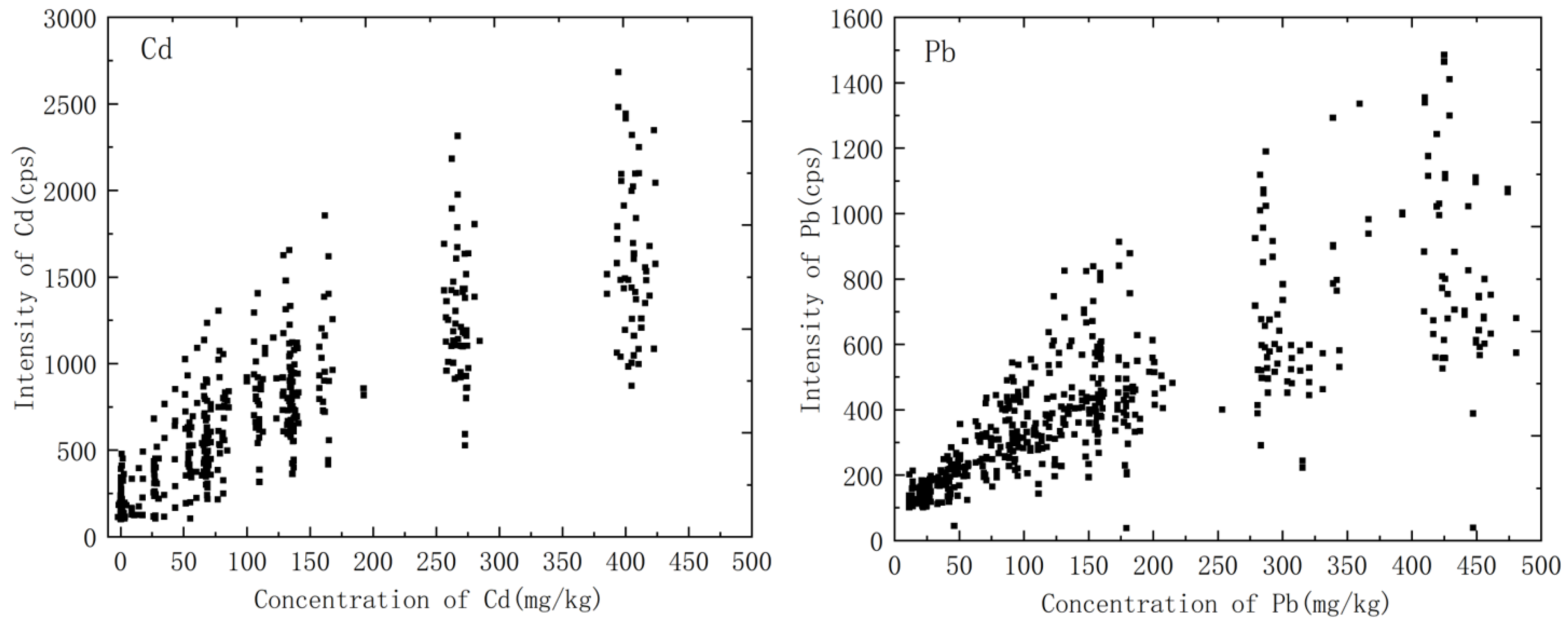
3.3.1. The Standard Soil Samples

Excluding the six standard samples used for calibration, 54 standard soil samples remained. Cd and Pb were added to part of these samples using the standard addition method, and then there were 78 samples in total. The concentrations of Cd and Pb were calculated using the corresponding calibration curves. The comparison between the prediction results of LIBS and the standard values are shown in Figure 6. The horizontal coordinate is the known heavy metal content, and the vertical coordinate is the concentration value detected by LIBS. The detection limits of Cd and Pb were, respectively, 3 and 10 mg·kg⁻¹ for this instrument. However, the Cd contents in 49 standard soil samples were very low, with a mean value of 0.14 mg·kg⁻¹, which were all below the detection limit of the instrument, and data below the detection limit were considered invalid. After the invalid datum were removed, there were 29 valid data for Cd. The 78 data for Pb were all valid. The square of the linear correlation coefficients R for Cd and Pb were 0.9730 and 0.9532, respectively. The average relative errors were 5.43% for Cd and 0.42% for Pb. The absolute error values were −43.21~56.88 mg·kg⁻¹ for Cd and −139.00~109.65 mg·kg⁻¹ for Pb, with averages of 3.09 mg·kg⁻¹ for Cd and 1.79 mg·kg⁻¹ for Pb. The root mean square error (RMSE) values were 16.45 mg·kg⁻¹ for Cd and 27.43 mg·kg⁻¹ for Pb. The results showed that the Cd and Pb contents in standard soils can be well predicted by the pre-classification method.

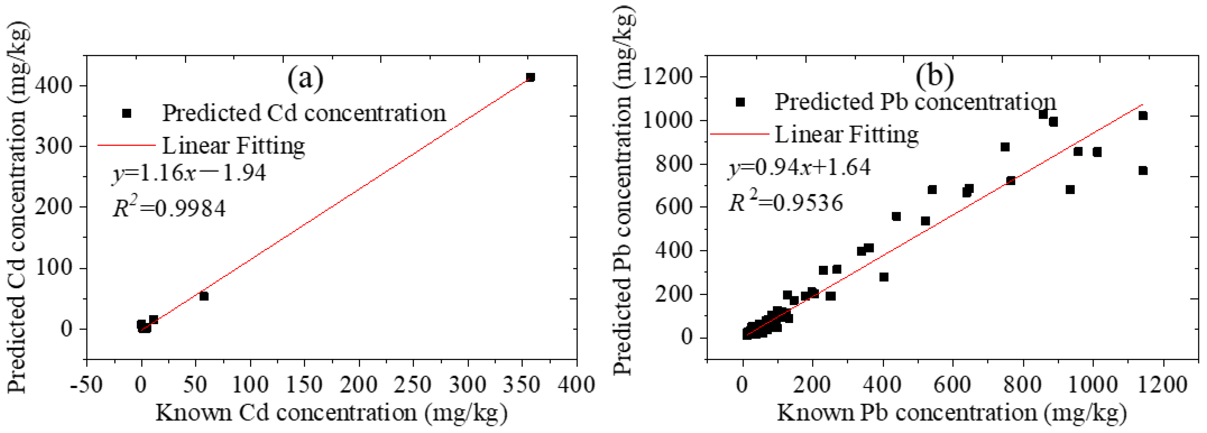
3.3.2. The Collected Soil Samples

For the soil samples collected from Tongling and Yunnan mining areas and Anhui Province, the comparisons between the prediction results of LIBS and the standard values are shown in Figure 7. There were only 11 valid data for Cd, because the Cd content in most soils was very low and could not be detected using this instrument, and there were 334 valid data for Pb.

The 11 soil samples were collected from Yunnan and Tongling mining areas. The two soil samples with the highest Cd content were collected from Tongling solid waste, and the Cd contents were 356.8 mg·kg⁻¹ and 57.08 mg·kg⁻¹, respectively. The Cd contents of the other nine samples were all below 11 mg·kg⁻¹. The square of the linear correlation coefficients R for Cd was 0.9984. The average of the absolute error was 4.56 mg·kg⁻¹, and the RMSE was 17.48 mg·kg⁻¹. Although the amount of Cd data was not sufficient, the results showed that the LIBS method is also comparable to the standard method.

For Pb content in the original soil samples, the sample from Tongling solid waste was the highest; the maximum value was 933.7 mg·kg⁻¹. The other four soil samples with the Pb content exceeding this value were prepared by adding Pb artificially. The square of R for Pb was 0.9536. The relative standard deviation was between −63.87% and 107.55%, with a mean of −2.35%. The RMSE was 17.48 mg·kg⁻¹. Ninety percent of the samples had a relative error of less than forty percent. The results indicated that the predicted values, which were calculated using the calibration model established by the pre-classification method based on the compactness of the soil pellets, were close to the true values. The number of samples with large errors accounted for 10%, which may have been caused by classification errors. Perhaps in addition to the compactness of the soil pellets, there were other factors that had greater impact on the spectrum. The Cd and Pb contents in soil could be quickly detected by this method. In practical application, the soils can be first classified according to the size of the ablation pit and the dust generated when the laser breaks down the soil samples, and then the samples can be calibrated using the corresponding calibration curve. This method did not require a large number of samples to establish models, and only a few gradient samples were required for one type of soil.

4. Conclusions and Prospects

The compactness of the soil pellets is closely related to laser ablation quality. This work attempted to classify soils according to the compactness of the soil pellets and then quantitatively analyze Cd and Pb in soils by the external standard method. The 451 soils were divided into six categories, and six calibration curves were made. The linear correlation coefficients were all above 0.98. In total, 78 standard soils and 334 collected soils were predicted, and the correlation coefficients were all above 0.95 compared with the results obtained using ICP-MS. This work demonstrated that the different soil matrix is largely reflected in the different ablative quality, which is one of the important factors to consider in quantitative analysis. However, the classification method in this paper was based on manual method and was subjective; individual sample error were large, most likely because of classification error. Subsequently, the classification of soil compactness can be realized by advanced means such as image recognition. On the other hand, we speculate that the compactness of the soil pellets is related to the content of organic matter in soil and hope to classify it by spectral signals in the future, rather than this subjective classification method. This can provide a new method for detecting elements in soil quickly and accurately using LIBS.

References

1. Wang, J.; He, Z.; Xie, S.; Liu, S. Health Risk Assessment of Heavy Metals (Pb, Cd, and Cr) in Farmland Soil of Hubei Province. J. Environ. Hyg. 2019, 9, 258–263. [Google Scholar]
2. Gong, D.C.L.; Zheng, H. Determination of Heavy Metals in Soil, Mushroom and Plant Samples by Atomic Absorption Spectrometry. Shandong Chem. Ind. 2020, 49, 101–103. [Google Scholar]
3. Li, H.; Gu, W.; Zhao, S.; Yang, M.; Wei, Z.; Zhou, N. Comparison of 6 heavy metal contents in Paris polyphylla Smith var.yunnanensis medicine and their rhizosphere soils from different geographical areas. Environ. Chem. 2021, 40, 2179–2192. [Google Scholar]
4. Meng, R.; Du, J.; Liu, Y.; Luo, L.; He, K.; Liu, M.; Liu, B. Exploration of Digestion Method for Determination of Heavy Metal Elements in Soil by ICP-MS. Spectrosc. Spectr. Anal. 2021, 41, 2122–2128. [Google Scholar]
5. Qasim, M.; Anwar-Ul-Haq, M.; Afgan, M.S.; Haq, S.U.; Baig, M.A. Quantitative analysis of saindha salt using laser induced breakdown spectroscopy and cross-validation with ICP-MS. Plasma Sci. Technol. 2020, 22, 074007. [Google Scholar] [CrossRef]
6. Wang, Z.; Afgan, M.S.; Gu, W.; Song, Y.; Wang, Y.; Hou, Z.; Song, W.; Li, Z. Recent advances in laser-induced breakdown spectroscopy quantification: From fundamental understanding to data processing. Trends Anal. Chem. 2021, 143, 116385. [Google Scholar]
7. Yan, C.; Qi, J.; Liang, J.; Zhang, T.; Li, H. Determination of coal properties using laser-induced breakdown spectroscopy combined with kernel extreme learning machine and variable selection. J. Anal. At. Spectrom. 2018, 33, 2089–2097. [Google Scholar] [CrossRef]
8. Jull, H.; Künnemeyer, R.; Schaare, P. Nutrient quantification in fresh and dried mixtures of ryegrass and clover leaves using laser-induced breakdown spectroscopy. Precis. Agric. 2018, 19, 823–839. [Google Scholar] [CrossRef]
9. Khalil, A.A.I.; Labib, O.A. Detection of micro-toxic elements in commercial coffee brands using optimized dual-pulsed laser-induced spectral analysis spectrometry. Appl. Opt. 2018, 57, 6729–6741. [Google Scholar]
10. Zhang, D.C.; Hu, Z.Q.; Su, Y.B.; Hai, B.; Zhu, X.L.; Zhu, J.F.; Ma, X. Simple method for liquid analysis by laser-induced breakdown spectroscopy (LIBS). Opt. Express 2018, 26, 18794–18802. [Google Scholar] [CrossRef]
11. Qi, J.; Zhang, T.; Tang, H.; Li, H. Rapid classification of archaeological ceramics via laser-induced breakdown spectroscopy coupled with random forest. Spectrochim. Acta B 2018, 149, 288–293. [Google Scholar] [CrossRef]
12. Bhatt, C.R.; Yueh, F.Y.; Singh, J.P. Univariate and multivariate analyses of rare earth elements by laser-induced breakdown spectroscopy. Appl. Opt. 2017, 56, 2280–2287. [Google Scholar] [CrossRef]
13. Gao, P.; Yang, P.; Zhou, R.; Ma, S.; Zhang, W.; Hao, Z.; Tang, S.; Li, X.; Zeng, X. Determination of antimony in soil using laser-induced breakdown spectroscopy assisted with laser-induced fluorescence. Appl. Opt. 2018, 57, 8942–8946. [Google Scholar] [CrossRef]
14. Mezzacappa, A.; Melikechi, N.; Cousin, A.; Wiens, R.; Lasue, J.; Clegg, S.; Tokar, R.; Bender, S.; Lanza, N.; Maurice, S.; et al. Application of distance correction to ChemCam laser-induced breakdown spectroscopy measurements. Spectrochim. Acta B 2016, 120, 19. [Google Scholar] [CrossRef]
15. Khalil, A.A.; Gondal, M.A.; Dastageer, M.A. Detection of trace elements in nondegradable organic spent clay waste using optimized dual-pulsed laser induced breakdown spectrometer. Appl. Opt. 2014, 53, 1709–1717. [Google Scholar] [CrossRef]
16. Ge, F.; Gao, L.; Peng, X.; Li, Q.; Zhu, Y.; Yu, J.; Wang, Z. Atmospheric pressure glow discharge optical emission spectrometry coupled with laser ablation for direct solid quantitative determination of Zn, Pb, and Cd in soils. Talanta 2020, 218, 121119. [Google Scholar] [CrossRef]
17. Umar, Z.A.; Liaqat, U.; Ahmed, R.; Baig, M.A. Detection of lead in soil implying sample heating and laser-induced breakdown spectroscopy. Appl. Opt. 2021, 60, 452–458. [Google Scholar] [CrossRef]
18. Dell’Aglio, M.; Gaudiuso, R.; Senesi, G.S.; De Giacomo, A.; Zaccone, C.; Miano, T.M.; De Pascale, O. Monitoring of Cr, Cu, Pb, V and Zn in polluted soils by laser induced breakdown spectroscopy (LIBS). J. Environ. Monit. 2011, 13, 1422–1426. [Google Scholar] [CrossRef]
19. He, Y.; Liu, X.; Lv, Y.; Liu, F.; Peng, J.; Shen, T.; Zhao, Y.; Tang, Y.; Luo, S. Quantitative Analysis of Nutrient Elements in Soil Using Single and Double-Pulse Laser-Induced Breakdown Spectroscopy. Sensors 2018, 18, 1526. [Google Scholar] [CrossRef]
20. Rühlmann, M.; Büchele, D.; Ostermann, M.; Bald, I.; Schmid, T. Challenges in the quantification of nutrients in soils using laser-induced breakdown spectroscopy—A case study with calcium. Spectrochim. Acta B 2018, 146, 115–121. [Google Scholar] [CrossRef]
21. Erler, A.; Riebe, D.; Beitz, T.; Löhmannsröben, H.-G.; Gebbers, R. Soil Nutrient Detection for Precision Agriculture Using Handheld Laser-Induced Breakdown Spectroscopy (LIBS) and Multivariate Regression Methods (PLSR, Lasso and GPR). Sensors 2020, 20, 418. [Google Scholar] [CrossRef]
22. Guo, G.; Niu, G.; Shi, Q.; Lin, Q.; Tian, D.; Duan, Y. Multi-element quantitative analysis of soils by laser induced breakdown spectroscopy (LIBS) coupled with univariate and multivariate regression methods. Anal. Methods 2019, 11, 3013. [Google Scholar] [CrossRef]
23. Liu, X.; Liu, F.; Huang, W.; Peng, J.; Shen, T.; He, Y. Quantitative determination of Cd in soil using laser-induced breakdown spectroscopy in Air and Ar conditions. Molecules 2018, 23, 2492. [Google Scholar] [CrossRef]
24. Bousquet, B.; Sirven, J.-B.; Canioni, L. Towards quantitative laser-induced breakdown spectroscopy analysis of soil samples. Spectrochim. Acta Part B 2007, 62, 1582–1589. [Google Scholar] [CrossRef]
25. Lu, C.; Wang, M.; Wang, L.; Hu, H.; Wang, R. Univariate and multivariate analyses of Sr and V in soil by laser-induced breakdown spectroscopy. Appl. Opt. 2019, 58, 7510–7516. [Google Scholar] [CrossRef]
26. Honawadm, S.K.; Chinchali, S.S.; Pawar, K.; Deshpande, P. Soil Classification and Suitable Crop Prediction. In Proceedings of the National Conference on Advances in Computational Biology, Communication, and Data Analytics; 2017; pp. 25–29. [Google Scholar]
27. Vrábel, J.; Képeš, E.; Duponchel, L.; Motto-Ros, V.; Fabre, C.; Connemann, S.; Schreckenberg, F.; Prasse, P.; Riebe, D.; Junjuri, R.; et al. Classification of challenging Laser-Induced Breakdown Spectroscopy soil sample data-EMSLIBS contest. Spectrochim. Acta Part B 2020, 169, 105872. [Google Scholar] [CrossRef]
Figure 1. Schematic of a portable LIBS system. (a) The core structure of spectral signal detection and sample control. (b) The portable on-site soil heavy metal laser-induced breakdown spectrum detector.
Chemosensors 12 00040 g001
Figure 2. Variation of spectral intensity of heavy metals in soil with concentration.
Chemosensors 12 00040 g002
Figure 3. (a) Photo of the soils after laser ablation; (b) microscopic photo of the ablative pits.
Chemosensors 12 00040 g003
Figure 4. Calibration curves of Cd and Pb for different categories of soils.
Chemosensors 12 00040 g004
Figure 5. Classification results of the soil samples.
Chemosensors 12 00040 g005
Figure 6. Prediction resultsof standard soils by LIBS (a) Cd and (b) Pb.
Chemosensors 12 00040 g006
Figure 7. Prediction results of collected soils by LIBS.
Chemosensors 12 00040 g007