L₁ Regularization for High-Dimensional Multivariate GARCH Models

Abstract

The complexity of estimating multivariate GARCH models increases significantly with the increase in the number of asset series. To address this issue, we propose a general regularization framework for high-dimensional GARCH models with BEKK representations, and obtain a penalized quasi-maximum likelihood (PQML) estimator. Under some regularity conditions, we establish some theoretical properties, such as the sparsity and the consistency, of the PQML estimator for the BEKK representations. We then carry out simulation studies to show the performance of the proposed inference framework and the procedure for selecting tuning parameters. In addition, we apply the proposed framework to analyze volatility spillover and portfolio optimization problems, using daily prices of 18 U.S. stocks from January 2016 to January 2018, and show that the proposed framework outperforms some benchmark models.

1. Introduction

Modeling the dynamics of high-dimensional variance–covariance matrices is a challenging problem in high-dimensional time series analysis and has wide applications in financial econometrics. Classical time series models for variance–covariance matrices assume that the number of component time series is low with respect to the number of observed samples. However, many financial and economic applications these days need to model the dynamics of high-dimensional variance–covariance matrices. For example, in modern portfolio management, the number of assets can easily be more than thousands and be larger or on the same order as the observed historical prices of the assets; in analyzing the movements in the financial markets of different products in different countries, it is critical to understand the interdependence and contagion effects of price movements over thousands of markets, while the amounts of jointly observed financial data are only available in decades.

In this paper, we propose an inference procedure with $L_1$ regularization for high-dimensional BEKK representations and obtain a class of penalized quasi-maximum likelihood (PQML) estimators. The $L_1$ regularization allows us to identify important parameters and shrink the non-essential ones to zero, hence providing an estimate of sparse parameters in BEKK representations. Under some regularity conditions, we establish some theoretical properties, such as the sparsity and the consistency, of the PQML estimator for BEKK representations. The proposed procedure is a fairly general framework that can be applied to a large class of high-dimensional MGARCH models; by applying our regularization techniques, the complexity of making inferences from high-dimensional MGARCH models can be greatly reduced and the intrinsic sparse model structures can be uncovered. We carried out simulation studies to show the performance of the proposed inference framework and the procedure for selecting tuning parameters. In addition, we applied the proposed framework to analyze volatility spillover and portfolio optimization problems, using daily prices of 18 U.S. stocks from January 2016 to January 2018. In the comparison of portfolio optimization based on different MGARCH models, we show that the proposed framework outperforms three benchmark models, i.e., the constant covariance model, the factor MGARCH model, and the dynamic conditional correlation model.

The proposed framework can be viewed as an extension of the literature on regularization techniques for converting high-dimensional linear models to nonlinear time series models. Since Tibshirani (1996) introduced LASSO for linear regression models, various regularization techniques concerning high-dimensional statistical inference have been studied for various problems in linear models. For example, Fan and Li (2001) proposed the smoothly clipped absolute deviation (SCAD) penalty that generates sparse estimation of regression coefficients with reduced bias and explored the so-called “oracle property”, in which the estimator has asymptotic properties that are equivalent to the maximum likelihood estimator in the non-penalized model. Zou (2006) proposed adaptive LASSO by adding adaptive weights for different parameters in the $L_1$ penalty to obtain better estimator performance. Yuan and Lin (2006) proposed a group LASSO penalty to solve the problem of selecting grouped factors in regression models. Zhang (2010) proposed a minimax concave penalty that gives nearly unbiased variable selection in linear regression. In addition to discussions on regularized estimation in high-dimensional statistics, which relies primarily on independent and identically distributed (i.i.d.) samples and linear models, regularization techniques have also been applied to study inference problems in high-dimensional linear time-series models. For instance, Uematsu (2015) studied a class of penalty functions and showed the oracle properties for the estimators in high-dimensional vector autoregressive (VAR) models. Basu and Michailidis (2015) investigated the theoretical properties of $L_1$-regularized estimates in high-dimensional stochastic regressions with serially correlated errors and transition matrix estimation in high-dimensional VAR models. Sun and Lin (2011) developed a regularization framework for full-factor MGARCH models (Vrontos et al. 2003), in which the dynamics of covariance matrices are determined by the dynamics of univariate GARCH processes for orthogonal factors. Using the group LASSO technique, Poignard (2017) studied the inference problem for MGARCH models with vine structure, an alternative to dynamic conditional correlation MGARCH models.

The proposed regularization framework is also related to the problem of estimating $p\times p$ covariance matrices using various shrinkage and regularization methods. For instance, Ledoit and Wolf (2004) proposed an optimal linear shrinkage method to estimate constant covariance matrices of p-dimensional i.i.d. vectors, and, later on, Ledoit and Wolf (2012) extended the method and developed nonlinear shrinkage estimators for high-dimensional covariance matrices. Bickel and Levina (2008) and Cai and Liu (2011) proposed covariance regularization procedures that are based on the thresholding of sample covariance matrices to estimate inverse covariance matrices. Lam and Fan (2009) studied sparsistency and rates of convergence for estimating covariance based on penalized likelihood with nonconcave penalties, and Ravikumar et al. (2011) estimated high-dimensional inverse covariance by minimizing $L_1$-penalized log-determinant divergence. This method is also called graphical LASSO and was studied in Yuan and Lin (2006) and Friedman et al. (2007). We note that all these discussions focus on high-dimensional constant covariance matrices; thus, they do not involve the dynamics of covariance matrices.

The remainder of the paper is organized as follows. Section 2 provides a literature review of MGARCH models and their applications in volatility spillover. Section 3 explains the BEKK model with $L_1$-penalty functions in detail. In Section 4, we provide theoretical properties and implementation procedures for the regularized BEKK model. Simulation results and real data analysis are presented in Section 5 and Section 6, respectively. Section 7 gives concluding remarks.

2. Literature Review

Inspired by the idea of univariate generalized autoregressive conditionally heteroskedastic (GARCH) models Bollerslev (1986); Engle (1982); Francq and Zakoian (2019); Hafner et al. (2022), various multivariate GARCH (MGARCH) models were proposed to characterize the dynamics of covariance matrices during the last three decades. Among these MGARCH models, the Baba–Engle–Kraft–Kroner (BEKK) model (Engle and Kroner 1995) uses a general specification to describe the dynamics of covariance matrices of an n-dimensional multivariate time series. Since such a specification contains unknown parameters of order $O\left(n^2\right)$, inference on the BEKK model becomes complicated, even for not very large ns. When $n^2$ increases with the same order as, or larger order than, the length of the time series, inference on the MGARCH–BEKK representation becomes even more difficult due to “the curse of dimensionality”.

To reduce the complexity of inference procedures for unknown parameters in MGARCH models, other forms of MGARCH specifications were proposed to reduce the number of unknown parameters in the model. An important improvement to MGARCH models is the dynamic conditional correlation (DCC) model (Aielli 2013; Bauwens and Laurent 2005; Boudt et al. 2013; Engle 2002). The DCC model allows for time-varying conditional correlations and reduces the dimensionality by factorizing the conditional covariance matrix into the product of a diagonal matrix of conditional standard deviations and a correlation matrix that evolves dynamically over time. Other forms of MGARCH specifications make more assumptions on structures and dynamics of covariance matrices and include, for example, the MGARCH in mean model (Bollerslev et al. 1988), the constant conditional correlation GARCH model (Bollerslev 1990; Ling and McAleer 2003; McAleer et al. 2009), the time-varying conditional correlation MGARCH model (Tse and Tsui 2002), the orthogonal factor MGARCH model (Hafner and Preminger 2009; Lanne and Saikkonen 2007), and so on. Although these MGARCH models provide relatively simple inference procedures, the assumptions on dynamics of covariance matrices are usually too specific to capture the complexity of dynamics of covariance matrices. Furthermore, these models still fail to address the issue of making inference on high-dimensional MGARCH models.

In addition to modeling the joint behavior of volatilities for a set of returns, another aspect of MGARCH models is to characterize volatility spillover in financial markets. Volatility spillover refers to as the process and magnitude by which the instability in one market affects other markets. Volatility spillover is widely observed in equity markets (Hamao et al. 1990), bond markets (Christiansen 2007), futures markets (Pan and Hsueh 1998), exchange markets (Baillie and Bollerslev 1990), markets of equities and exchanges (Apergis and Rezitis 2001), various industries and commodities (Apergis and Rezitis 2003; Kaltenhäuser 2002), and so on. Understanding volatility spillover can provide an insight into financial vulnerabilities, as well as the source and nature of financial exposures, for academic researchers, financial practitioners, and regulatory authorities. For investors, as significant volatility spillover may increase non-systemic risk, understanding volatility spillover can help them diversify the risks associated with their investment. For financial sector regulators, understanding volatility spillover can help them formulate appropriate policies to maintain financial stability, especially when stress from a particular market is transmitted to other markets, such that the risk of systemic instability increases. MGARCH models are generally used to characterize volatility spillover in the markets, which are represented via a low-dimensional multivariate series; see Hamao et al. (1990), Christiansen (2007); Pan and Hsueh (1998), Engle et al. (1990), and Baillie and Bollerslev (1990). In particular, Theodossiou and Lee (1993) used multivariate GARCH-in-mean model to study the economic spillover effect across five countries, Worthington and Higgs (2004) applied a BEKK(1,1) model to study transmission of weekly equity returns and volatility in nine Asian countries from 1988 to 2000, and Hassan and Malik (2007) employed the BEKK(1,1) specification to study three-dimensional US sector indices. Spillover effect has also been explored recently for other financial markets, such as cryptocurrency markets (Billio et al. 2023) and European banks with GARCH models (Giacometti et al. 2023). Additionally, there has been an investigation into the spillover effects using network representations derived from GARCH models in recent studies (Ampountolas 2022; Hong et al. 2023).

The aforementioned studies on spillover effects rely on the foundational structures of the DCC model for analysis (Ampountolas 2022; Shiferaw 2019; Siddiqui and Khan 2018). Although these MGARCH models provide relatively simple inference procedures, the assumptions on dynamics of covariance matrices are usually too specific to capture the complexity of the dynamics of covariance matrices. Moreover, these models still fail to address the issue of making inference on high-dimensional MGARCH models. Under these constraints, the performance and accuracy of these simplified MGARCH models need further investigation in real markets (Engle and Colacito 2006).

3. The MGARCH–BEKK Representations with $L_1$ Regularization

We first introduce the following notations. Given a vector x and a matrix A, the ith component of x and the $ij$th elements of A are written as $x_i$ and $A_{ij}$, respectively. The jth column and the ith row vectors of A are denoted as $A_{.j}$ and $A_{i.}$, respectively. $\left|\right|x\left|\right|$ is the Euclidean norm for vector x. ${\left|\right|x\left|\right|}_{\infty }$ is the largest element of x in the modulus. $\rho \left(A\right)$ is the spectral radius of A, i.e., the largest modulus of eigenvalues of A. ${\lambda }_{min}\left(A\right)$ and ${\lambda }_{\max }\left(A\right)$ are the minimum and maximum eigenvalues of A, respectively. $\left|\right|A\left|\right|$ is the spectral norm, i.e., a square root of $\rho \left(A^{T}A\right)$. ${\left|\right|A\left|\right|}_{\infty }$ represents the operator norm induced by ${\left|\right|x\left|\right|}_{\infty }$, or the largest absolute row sum. For any matrix A and vector x such that $Ax$ is well defined, let ${\left|\right|A\left|\right|}_{2,\infty }:={\max }_{\left|\right|x\left|\right|=1}{\left|\right|Ax\left|\right|}_{\infty }$. We use $\mathrm{sign}\left(x\right)$ to denote the sign of $x:\mathrm{sign}\left(x\right)=x/\left|x\right|$ if $x\ne 0$, and $\mathrm{sign}\left(x\right)=0$ otherwise.

3.1. The MGARCH–BEKK Representation

Let $r_t$ be the vector of returns on n assets in period t. Let ${ϵ}_t$ be i.i.d. n-dimensional standard normal random vectors. Let ${\mathcal{F}}_t$ be the sigma field generated by the past information from $r_t$s. Then, ${\Sigma }_t$ is measurable with respect to ${\mathcal{F}}_{t-1}$; the distribution of $r_t$ can be specified as

$$r_t={\Sigma }_t^{-\frac{1}{2}}{ϵ}_t,{ϵ}_t\sim N(0,I_n),$$

(1)

where $I_n$ is an $n\times n$ identity matrix. Denote the conditional covariance matrix of $r_t$ given ${\mathcal{F}}_{t-1}$ as ${\Sigma }_t$, i.e., ${\Sigma }_t=\mathrm{Cov}\left(r_t\right|{\mathcal{F}}_{t-1})$. Engle and Kroner (1995) proposed the following BEKK$(a,b)$ model to characterize the dynamics of ${\Sigma }_t$:

$${\Sigma }_t=C^{\prime }C+\sum _{k=1}^K\sum _{i=1}^a{A}_{ik}{r}_{t-1}{r}_{t-1}^{\prime }{A}_{ik}^{\prime }+\sum _{k=1}^K\sum _{i=1}^b{B}_{ik}{\Sigma }_{t-1}{B}_{ik}^{\prime },$$

(2)

where $A_{ik}$, and $B_{ik}$ are $n\times n$ parameter matrices, C is an $n\times n$ triangular matrix, and the summation limit K determines the generality of the process.

To illustrate the idea, we consider BEKK(1,1) in our examples with $K=1$ in this paper, which can be written as

$${\Sigma }_t=C^{\prime }C+\sum _{i=1}^a{A}_i{r}_{t-i}{r}_{t-i}^{\prime }{A}_i^{\prime }+\sum _{i=1}^b{B}_i{\Sigma }_{t-i}{B}_i^{\prime }.$$

(3)

in which $A_i,$$B_i$, and C are real $n\times n$ matrices. And, without loss of generality, we choose ${\Sigma }_t^{-1/2}$ to be symmetric. For identification purposes, Engle and Kroner (1995) showed the following property for the BEKK model.

Proposition 1.

Suppose that the diagonal elements in C, $a_{11}$, and $b_{11}$ are positive. Then, there exists no other C, A, or B in Model (3) that gives an equivalent representation.

Proposition 1 is also known as the identification condition (Comte and Lieberman 2003).

Let vec and vech be the vector operators that stack the columns of a matrix and the lower triangular part of a matrix, respectively. That is, if

$$Y=\left(\begin{array}{ccc}{y}_{11}& \cdots & y_{1n}\\ ⋮& \ddots & ⋮\\ y_{n1}& \cdots & y_{nn}\end{array}\right),$$

then

$$vec\left(Y\right)={(y_{11},\cdots ,y_{n1},y_{12},\cdots ,y_{n2},\cdots ,y_{1n},\cdots ,y_{nn})}^{\prime },$$

and

$$vech\left(Y\right)={(y_{11},\cdots ,y_{n1},y_{22},\cdots ,y_{n2},\cdots ,y_{ii},\cdots ,y_{in},\cdots y_{nn})}^{\prime }.$$

Then, Model (3) can be rewritten in a vector form:

$$vec\left({\Sigma }_t\right)=vec\left(C^{\prime }C\right)+\sum _{i=1}^a\mathring{A_i}vec\left(r_{t-i}{r}_{t-i}^{\prime }\right)+\sum _{i=1}^b\mathring{B_i}vec\left({\Sigma }_{t-i}\right).$$

(4)

in which $\mathring{A_i}=A_i\otimes A_i$, $\mathring{B_i}=B_i\otimes B_i$, and ⊗ is the Kronecker product. Since the covariance matrices ${\Sigma }_t$ are symmetric, we can also write (3) in the vector-half form:

$$vech\left({\Sigma }_t\right)=vech\left(C^{\prime }C\right)+\sum _{i=1}^a{\tilde{A}}_{i}vech\left(r_{t-i}{r}_{t-i}^{\prime }\right)+\sum _{i=1}^b{\tilde{B}}_{i}vech\left({\Sigma }_{t-i}\right).$$

(5)

where $\widetilde{A_i}=L_n\mathring{A_i}{K}_n^{\prime }$, $\widetilde{B_i}=L_n\mathring{B_i}{K}_n^{\prime }$, and $L_n$ and $K_n$ are matrices of dimension $n(n+1)\times n^2$ extracting the upper triangular parts of symmetric matrices $\mathring{A_i}$ and $\mathring{B_i}$. Note that dim$\left(vec\left({\Sigma }_t\right)\right)=n^2$ and dim$\left(vech\left({\Sigma }_t\right)\right)=n(n+1)/2$. For convenience, we denote $\theta ={({\theta }_1,\cdots ,{\theta }_p)}^{\prime }$ by the parameter vector in Model (3), in which $p=2(a+b)n^2+n(n+1)/2$, so that the matrices C, $A_i$, and $B_i$ are functions of $\theta$: $C=C\left(\theta \right),A_i=A_i\left(\theta \right),B_i=B_i\left(\theta \right)$. And we denote by ${\theta }^0$ the true parameter vector of the model.

We assume that the values of $r_t$ in (1) are stationary; then, the following stationary condition should be imposed for the BEKK$(a,b)$ Model (5) (see Engle and Kroner (1995) and Comte and Lieberman (2003)).

Condition 1 (Stationary Condition).

The p-dimensional return series $r_t$ in (1) is stationary if the following conditions hold for Model (3):

(i) 

$C^{*}\left(\theta \right)=C^{\prime }C$ is a continuous function of $\theta$, and there exists $C_0>0$, $det\left(C^{*}\left(\theta \right)\right)\ge C_0$, where $det(·)$ represents the determinant of a matrix;

(ii) 

For any $\theta$, ${\tilde{A}}_i\left(\theta \right)$ and $\widetilde{B_i}\left(\theta \right)$ are continuous functions of $\theta$;

(iii) 

For any $\theta$, $\rho ({\sum }_{i=1}^a{\tilde{A}}_i\left(\theta \right)+{\sum }_{i=1}^b{\tilde{B}}_i\left(\theta \right))<1$, i.e., the largest modulus of eigenvalues of ${\sum }_{i=1}^a{\tilde{A}}_i\left(\theta \right)+{\sum }_{i=1}^b{\tilde{B}}_i\left(\theta \right)$ is less than 1.

3.2. Likelihood Function

In this section, we discuss some properties of the likelihood of the BEKK$(a,b)$ model. Assume that ${ϵ}_t$ follows a standard n-dimensional Gaussian distribution. Ignoring constants, we can write the quasi-log-likelihood as

$${\ell }_T\left(\theta \right)=\frac{1}{2T}\sum _{t=1}^T{l}_t\left(\theta \right),l_t\left(\theta \right)=-(\log \left[det\left({\Sigma }_t\right)\right]+r_t^{\prime }{\Sigma }_t^{-1}{r}_t).$$

(6)

Taking the derivative on ${\Sigma }_t$ with respect to the ith element of $\theta$, we obtain

$$\begin{array}{ccc}& & \frac{\partial {\Sigma }_t}{\partial {\theta }_i}=\frac{\partial C^{\prime }C}{\partial {\theta }_i}+\sum _{j=1}^a\left(\frac{\partial A_j}{\partial {\theta }_i}{r}_{t-j}{r}_{t-j}^{\prime }{A}_j^{\prime }+A_j{r}_{t-j}{r}_{t-j}^{\prime }\frac{\partial A_j^{\prime }}{\partial {\theta }_i}\right)+\sum _{j=1}^b(\frac{\partial B_j}{\partial {\theta }_i}{\Sigma }_{t-j}{B}_j\hfill \\ & & +B_j{\Sigma }_{t-j}\frac{\partial B_j^{\prime }}{\partial {\theta }_i}+B_j\frac{\partial {\Sigma }_{t-j}}{\partial {\theta }_i}{B}_j^{\prime }),\hfill \end{array}$$

(7)

which can be computed recursively. The derivative in (7) has the following property (the proof is given in Appendix A).

Proposition 2.

Let ${\mathfrak{R}}_t=vech\left(r_t{r}_t^{\prime }\right)$; then,

$$∥\frac{\partial {\Sigma }_t}{\partial {\theta }_i}∥\le {\Psi }_1+{\Psi }_2·sup\left|\right|{\mathfrak{R}}_t\left|\right|.$$

where ${\Psi }_1$ and ${\Psi }_2$ are two constants.

Assume that $L_T\left(\theta \right)$ is twice continuously differentiable in a neighborhood ${\Theta }^0\in \Theta$ of ${\theta }^0.$ We define the averages of the score vector and Hessian matrix as follows:

$$S_T\left(\theta \right)=T^{-1}\sum _{t=1}^T{s}_t\left(\theta \right)\mathrm{and}{H}_T\left(\theta \right)=T^{-1}\sum _{t=1}^T{h}_t\left(\theta \right),$$

where $s_t\left(\theta \right)=\partial l_t\left(\theta \right)/\partial \theta$ and $h_t\left(\theta \right)={\partial }^2{l}_t\left(\theta \right)/\partial \theta \partial {\theta }^{\prime }$. Taking the derivative of (6) with respect to ${\theta }_i$ yields

$$\frac{\partial l_t}{\partial {\theta }_i}=-Tr\left(\frac{\partial {\Sigma }_t}{\partial {\theta }_i}{\Sigma }_t^{-1}-r_t{r}_t^{\prime }{\Sigma }_t^{-1}\frac{\partial {\Sigma }_t}{\partial {\theta }_i}{\Sigma }_t^{-1}\right),$$

$$\begin{array}{ccc}\hfill \frac{{\partial }^2{l}_t\left(\theta \right)}{\partial {\theta }_j\partial {\theta }_i}& =& -Tr\left(\frac{{\partial }^2{\Sigma }_t}{\partial {\theta }_j\partial {\theta }_i}{\Sigma }_t^{-1}-\frac{\partial {\Sigma }_t}{\partial {\theta }_i}{\Sigma }_t^{-1}\frac{\partial {\Sigma }_t}{\partial {\theta }_j}{\Sigma }_t^{-1}+r_t{r}_t^{\prime }{\Sigma }_t^{-1}\frac{\partial {\Sigma }_t}{\partial {\theta }_j}{\Sigma }_t^{-1}\frac{\partial {\Sigma }_t}{\partial {\theta }_i}{\Sigma }_t^{-1}\right.\hfill \\ & & \left.-r_t{r}_t^{\prime }{\Sigma }_t^{-1}\frac{{\partial }^2{\Sigma }_t}{\partial {\theta }_j\partial {\theta }_i}{\Sigma }_t^{-1}+r_t{r}_t^{\prime }{\Sigma }_t^{-1}\frac{\partial {\Sigma }_t}{\partial {\theta }_i}{\Sigma }_t^{-1}\frac{\partial {\Sigma }_t}{\partial {\theta }_j}{\Sigma }_t^{-1}\right),\hfill \end{array}$$

in which $Tr(·)$ represents the trace of a matrix. Comte and Lieberman (2003) showed the following property for $l_t\left(\theta \right)$.

Proposition 3.

Under Condition 1, the following properties hold:

(i) 

When $T\to +\infty$, $-H_T^0:=-{\displaystyle \frac{1}{T}\sum _{t=1}^T\frac{\partial l_t^2\left({\theta }^0\right)}{\partial \theta \partial {\theta }^{\prime }}\stackrel{P}{\to }H}$ for a nonrandom positive-definite matrix H;

(ii) 

For the Fisher information matrix $I_0:=E({\displaystyle \frac{\partial l_t\left({\theta }^0\right)}{\partial \theta }·\frac{\partial l_t\left({\theta }^0\right)}{\partial {\theta }^{\prime }})}$ $=E\left(S_T^0{\left(S_T^0\right)}^{\prime }\right)$, $\left|\right|I_0{\left|\right|}_{\infty }<\infty$;

(iii) 

For $\theta \in \Theta$, $E\left({sup}_{\left|\right|\theta -{\theta }^0\left|\right|\le ϵ}\right|{\displaystyle \frac{{\partial }^3{l}_t\left(\theta \right)}{\partial {\theta }_i\partial {\theta }_j\partial {\theta }_k}\left|\right)}$ is bounded for all $ϵ>0$ and $i,j,k=1,\dots ,p$.

In the sparse representation, the majority elements of the true parameter vector ${\theta }^0$ are exactly 0. Hence, we could partition ${\theta }^0$ into two sub-vectors. Let ${\mathcal{U}}_0$ be the set of indices $\{j\in \{1,\dots ,p\}:{\theta }_j^0\ne 0\}$ and ${\theta }_{{\mathcal{U}}_0}^0$ be the q-dimensional vector composed of the nonzero elements $\{{\theta }_j^0\ne 0:j\in {\mathcal{U}}_0\}.$ Similarly, we define ${\theta }_{{\mathcal{U}}_0^c}^0$ as a $(p-q)$-dimensional zero vector. Without loss of generality, ${\theta }^0$ is stacked as ${\theta }^0=({\left({\theta }_{{\mathcal{U}}_0}^0\right)}^{\prime },0^{\prime })=({\left({\theta }_{{\mathcal{U}}_0}^0\right)}^{\prime },{\left({\theta }_{{\mathcal{U}}_0^c}^0\right)}^{\prime })$. For convenience, we define the average of the “score subvector” $S_{{\mathcal{U}}_0,T}\left(\theta \right)$ and the “Hessian sub-matrix” $H_{{\mathcal{U}}_0,T}\left(\theta \right)$ by $s_{{\mathcal{U}}_0,t}\left(\theta \right)=\partial l_t\left(\theta \right)/\partial {\theta }_{{\mathcal{U}}_0}$ and $h_{{\mathcal{U}}_0,t}\left(\theta \right)={\partial }^2{l}_t\left(\theta \right)/\partial {\theta }_{{\mathcal{U}}_0}\partial {\theta }_{{\mathcal{U}}_0}^{\prime }$. Similarly, we define $S_{{\mathcal{U}}_0^c,T}\left(\theta \right)$. We also denote $S_T\left({\theta }^0\right)=S_T({\theta }_{{\mathcal{U}}_0}^0,0)$ as $S_T^0.$

Proposition 4.

The quasi-log-likelihood function $L_T$ for the BEKK(1,1) has the following properties:

(i) 

For $i=1,\dots ,p$, $E\left(|T·S_{T,i}^0{|}^4\right)<\infty$, where $S_{T,i}^0$ is the ith element of $S_T^0$;

(ii) 

For a sufficiently large T, $-H_{{\mathcal{U}}_0,T}^0$ is almost surely positive definite, and ${\lambda }_{min}(-H_{{\mathcal{U}}_0,T}^0)=O_p\left(1\right);$

(iii) 

There exists a neighborhood ${\Theta }_{{\mathcal{U}}_0}^0\subset \Theta$ of ${\theta }_{{\mathcal{U}}_0}^0$ such that, for all ${\theta }^{\left(1\right)}$ and ${\theta }^{\left(2\right)}\in {\Theta }_{{\mathcal{U}}_0}^0$ and some $K_T=O_p\left(1\right)$,

$$\left|\right|H_{{\mathcal{U}}_0,T}({\theta }^{\left(1\right)},0)-H_{{\mathcal{U}}_0,T}({\theta }^{\left(2\right)},0)\left|\right|\le K_T\left|\right|{\theta }^{\left(1\right)}-{\theta }^{\left(2\right)}\left|\right|.$$

Here, $a_T=O_p\left(1\right)$ means that $|a_T|\le c$ with probability 1 when $T\to \infty$ and c is a constant. Proposition 4(i) shows that the fourth moment of the score function $S_T$ is always finite. Proposition 4(ii) indicates that ${\lambda }_{min}(-H_{{\mathcal{U}}_0,T}^0)$ is almost surely positive and bounded away from 0. Hence, when the $L_1$ penalty is combined with the quasi-likelihood function, the concavity around ${\theta }^0$ can be ensured, so that a local maximizer can be obtained. Proposition 4(iii) is trivial in linear models, but not in our case. The proof of Proposition 4 is given in Appendix A.

3.3. $L_1$ Penalty Function and Penalized Quasi-Likelihood

Before discussing the consistency of the sparse estimator, we introduce the following condition, by following the strong irrepresentable condition for LASSO-regularized linear regression models in Zhao and Yu (2006).

Condition 2 (Irrepresentable condition).

There exists a neighborhood ${\Theta }_{{\mathcal{U}}_0}^0\subset \Theta$ of ${\theta }_{{\mathcal{U}}_0}^0$, such that

$$\underset{{\theta }^{\left(1\right)},{\theta }^{\left(2\right)}\in {\Theta }_{{\mathcal{U}}_0}^0}{sup}\left|\right|\left[(\partial /\partial {\theta }_{{\mathcal{U}}_0}^T)S_{{\mathcal{U}}_0^c,T}({\theta }^{\left(1\right)},0)\right]{\left[H_{{\mathcal{U}}_0,T}({\theta }^{\left(2\right)},0)\right]}^{-1}{\left|\right|}_{\infty }\le c$$

for a constant c that takes its value in (0,1) almost surely.

Definition 1.

The half of the minimum signal d is defined as

$$d(d=d_T)=\frac{1}{2}min\left\{\right|{\theta }_j^0| : {\theta }_j^0\ne 0\}=\frac{1}{2}\underset{j\in {\mathcal{U}}_0}{min}\left|{\theta }_j^0\right|.$$

(8)

Assume that $p_{\lambda }\left(x\right)$ is an $L_1$ penalty function, i.e., $p_{\lambda }\left(\right|x\left|\right)=\lambda \left|x\right|$. We consider the following penalized quasi-likelihood (PQL):

$$Q_T\left(\theta \right)=L_T\left(\theta \right)-P_T\left(\theta \right)$$

(9)

in which $P_T\left(\theta \right)={\sum }_{j=1}^p{p}_{\lambda }\left(\right|{\theta }_j\left|\right)=\lambda {\sum }_{j=1}^p\left|{\theta }_j\right|$ is the penalty term and $\lambda (={\lambda }_T)\ge 0$ is the regularization parameter determining the size of the model. If $\widehat{\theta }$ maxmizes the PQL, i.e.,

$$\widehat{\theta }=arg\underset{\theta \in \Theta }{\max }{Q}_T\left(\theta \right).$$

we say that $\widehat{\theta }$ is a penalized quasi-maximum likelihood estimator (PQMLE).

Similar to Fan and Lv (2011) and Uematsu (2015), we add some conditions on the penalty function $p_{\lambda }(·)$ and the half minimum signal.

Condition 3.

The penalty function $p_{\lambda }$ satisfies the following properties:

(i) 

$\lambda =min\{O\left(T^{-\alpha }\right),o\left(q^{-\frac{1}{2}}{T}^{-\gamma }\log T\right)\}$ for some $\alpha \in ({\delta }_0+\gamma ,\frac{1}{2}-\frac{{\delta }_0}{4})$, $\gamma \in (0,\frac{1}{2}]$ and large T. Here, $a=O\left(f\right(T\left)\right)$ means $|a/f(T\left)\right|$ is bounded by a constant and $b=o\left(g\right(T\left)\right)$ means $|b/g(T\left)\right|\to$ when $T\to \infty$;

(ii) 

$d\ge T^{-\gamma }\log T$ for some $\gamma \in (0,\frac{1}{2}]$ and large T, where d is the half-minimum signal we defined before.

4. Properties of the PQML Estimator and Implementation

This section studies the sparsity and the consistency of the PQML estimator and discuss some implementation issues.

4.1. Sparsity of the PQML Estimator

First, we introduce three lemmas whose proofs are given in Appendix A. For convenience, we denote $\widehat{\mathcal{U}}:=\mathrm{supp}\left(\widehat{\theta }\right)$, which is a set of indices corresponding to all nonzero components of $\widehat{\theta }$, where supp is the notation of support set and ${\widehat{\theta }}_{\widehat{\mathcal{U}}}$ is a subvector of $\widehat{\theta }$, formed by its restriction to $\widehat{\mathcal{U}}$. Then, $\widehat{{\mathcal{U}}^c}$ represents a set of indices corresponding to all 0 components in $\widehat{\theta }$. We also denote ⊙ as the Hadmard product.

Lemma 1.

When the penalty function $p_{\lambda }$ satisfies Condition 3, $\widehat{\theta }$ is a strict local maximizer of the $L_1$-PQL $Q_T\left(\theta \right)$ defined in (9) if

$$\begin{array}{ccc}& & S_{\widehat{\mathcal{U}},T}\left(\widehat{\theta }\right)-{\lambda }_T\mathbf{1}\odot sign\left({\widehat{\theta }}_{\widehat{\mathcal{U}}}\right)=0,\hfill \end{array}$$

(10)

$$\begin{array}{ccc}& & \left|\right|S_{\widehat{{\mathcal{U}}^c},T}\left(\widehat{\theta }\right){\left|\right|}_{\infty }<{\lambda }_T,\hfill \end{array}$$

(11)

$$\begin{array}{ccc}& & {\lambda }_{min}[-H_{\widehat{\mathcal{U}},T}\left(\widehat{\theta }\right)]>0,\hfill \end{array}$$

(12)

in which $\mathbf{1}$ represents the vector with all elements equaling to 1 and $sign(·)$ is as defined at the beginning of Section 3.

To show the weak oracle property of the PQML estimator, we also need the following lemma.

Lemma 2.

Let $w_t$ be a martingale difference sequence with $E|w_t{|}^m\le C_w$ for all t, where $m>2$ and $C_w$ is a constant. Then, we have

$$T^{-\frac{m}{2}}E{\left(\sum _{t=1}^T{w}_t\right)}^m<\infty .$$

Then, the weak oracle property of the PQML estimator can be established by the following theorem, whose proof is provided in Appendix A.

Theorem 1.

($L_1$-PQML estimator) Under Conditions 2 and 3, for the $L_1$ penalty function $P_T\left(\theta \right)=\lambda {\sum }_{i=1}^p\left|\theta \right|$, in which $p=O\left(T^{\delta }\right)$ and $q=O\left(T^{{\delta }_0}\right)$, if

$$\delta \in [0,4(\frac{1}{2}-\alpha )),0<{\delta }_0<min\{\frac{2}{3}(1-2\gamma ),\gamma \},$$

with $\alpha \in ({\delta }_0+\gamma ,\frac{1}{2}-\frac{{\delta }_0}{4})$, $\gamma \in (0,\frac{1}{2}],$ and $\delta >{\delta }_0$, then there exists a local maximizer $\widehat{\theta }={({\left({\widehat{\theta }}_{{\mathcal{U}}_0}\right)}^{\prime },{\left({\widehat{\theta }}_{{\mathcal{U}}_0^c}\right)}^{\prime })}^{\prime }$ for $Q_T\left(\theta \right)$, such that the following properties are satisfied:

(i) 

(Sparsity) ${\widehat{\theta }}_{{\mathcal{U}}_0^c}=0$ with probability approaching one;

(ii) 

(Rate of convergence) $\left|\right|{\widehat{\theta }}_{{\mathcal{U}}_0}-{\theta }_{{\mathcal{U}}_0}^0{\left|\right|}_{\infty }=O_p\left(T^{-\gamma }\log T\right).$

$p=O\left(T^{\delta }\right)$ is equivalent to $\frac{p}{T^{\delta }}\le c$ when $T\to \infty$. The growth rate of p is controlled by $T^{\delta }$ and q is slower than with $T^{{\delta }_0}$. For example, to make this growth rate of q much slower than p, we can find a set of values for $\delta =\frac{3}{2},$ ${\delta }_0=\frac{1}{20},$ $\gamma =\frac{1}{30}$, and $\alpha =\frac{1}{5}$ that satisfy the conditions above. Since, in our case, $p\sim O\left(n^2\right)$, we have $n=O\left(T^{\frac{3}{4}}\right)$ and, hence, it is possible for n to exceed the sample size T. Although the difference between the rates of p and n is not as large as that in (Fan and Lv 2011), in which $\log p=O\left(T^{1-2\alpha }\right)$ and $q=o\left(T\right)$, it is enough to be applied in most cases in practice.

4.2. Implementation and Selection of $\lambda$

To compute the whole regularization path of $L_1$-PQML estimators, we note that several algorithms have been proposed to solve penalized optimization problems. For example, Efron et al. (2004) proposed the least-angle regression (LARS) algorithm to compute an efficient solution to the optimization problem for LASSO. Later on, pathwise coordinate descent methods were proposed to solve the LASSO-type problem efficiently; see Friedman et al. (2007) and Wu and Lange (2008). For the PQML estimator, we used an algorithm inspired by the BLasso algorithm (Zhao and Yu 2006, 2007) with some necessary modifications since the BLasso algorithm does not need to explicitly calculate the first derivatives and second derivatives of the likelihood function, which are complicated in our case. We note that the original BLasso algorithm uses 0 as initial values for all parameters, but the diagonal elements of A and B are positive by definition, so we make the following modification. We set 0 as the initial values for all off-diagonal elements in A, B, and C, and set the estimated values of fitting the component series into a univariate GARCH model as the initial values of the diagonal elements in parameter matrices A, B, and C.

Another issue in the implementation is to select the tuning parameter $\lambda$, which leads to the problem of model selection. The tuning parameter $\lambda$ can be chosen by several criteria. For example, it is usually easy to consider the Akaike information criterion (AIC), the small-sample corrected AIC (AICC), and Bayesian information criterion (BIC) criteria to select the tuning parameter. In addition, Wang et al. (2009) proposed a modified BIC criterion and Fan and Tang (2013) extended it for the case $p>T$. Sun et al. (2013) proposed using Cohen’s kappa coefficient, which measures the agreement between two sets. Another method for model selection is to use cross-validation (CV). Zhang and Yang (2015) used CV to choose the best model among model selection procedures such as AIC and BIC. In our study, we apply the AIC and BIC criteria on the testing data and select the best tuning parameters. Note that, since our data are ordered, k-fold CV is not applicable here and the data are split in time order.

5. Simulation

In this section, we study the performance of the regularized BEKK models on some simulated examples. Consider Model (3) with $n=4$ and $a=b=1$. Note that we then have $p=42$ parameters, as matrix C is lower triangular. We assume that the parameter matrices satisfy the stationary condition, Condition 2, and, for identification purposes, we assume that the diagonal elements in C are positive, $a_{11}>0$, and $b_{11}>0$. We consider two cases for matrices A, B, and C, which are summarized in Table 1. In both cases, the indices of nonzero elements in coefficient matrices A, B, and C are randomly generated. To ensure that the matrices satisfy Condition 1, values of the diagonal elements in A and B are randomly generated from a uniform distribution on U$(-0.45,0.45)$, and the off-diagonal nonzero elements in A and B are generated from U$(-0.5,0.5)$. All the nonzero elements in C are generated from U$(-0.1,0.1)$.

Table 1. Parameter matrices in simulations.

	Case 1	Case 2
A	$\left(\begin{array}{cccc}0.1268& 0& 0.0358& -0.0618\\ 0& 0.1737& 0& 0\\ 0& 0& 0.2621& 0\\ 0& 0& 0& 0.4096\end{array}\right)$	$\left(\begin{array}{cccc}0.4040& -0.0200& 0& 0\\ 0& 0.4434& -0.0752& 0\\ 0& 0& 0.0406& 0.0684\\ 0& 0& 0& 0.2226\end{array}\right)$
B	$\left(\begin{array}{cccc}0.4257& 0& 0& 0\\ 0& 0.3008& 0& 0\\ 0.0912& 0& 0.2868& 0\\ 0& 0& 0& 0.0372\end{array}\right)$	$\left(\begin{array}{cccc}0.2453& 0& 0& 0\\ 0& 0.2401& 0& 0\\ 0.2398& 0& 0.2157& 0\\ 0& 0& 0& 0.3996\end{array}\right)$
C	$\left(\begin{array}{cccc}0.0324& 0& 0& 0\\ 0& 0.0681& 0& 0\\ 0& 0.0349& 0.0469& 0\\ 0.0728& 0& 0& 0.0739\end{array}\right)$	$\left(\begin{array}{cccc}0.0804& 0& 0& 0\\ 0& 0.0473& 0& 0\\ 0& 0& 0.0521& 0\\ 0.0200& 0& 0& 0.0628\end{array}\right)$

For each case, we simulate the data $r_t$$(1\le t\le T)$ with $T=600$, and then use the proposed regularized procedure to make inference on the model. Since the diagonal elements in A, B, and C cannot be zero, we do not shrink the diagonal elements in A, B, and C. Additionally, we set the estimates of parameters in univariate GARCH models for each component series as the initial values of diagonal elements in A, B, and C.

To demonstrate the performance of our estimates, we consider three measurements. The first is the success rate in estimating zero and nonzero elements in $\theta$ or parameter matrices:

$${\tau }_0=\frac{{\sum }_{i=1}^{p}I({\theta }_i^0=0\wedge {\widehat{\theta }}_i=0)}{{\sum }_{i=1}^{p}I({\theta }_i^0=0)},{\tau }_{0^C}=\frac{{\sum }_{i=1}^{p}I({\theta }_i^0\ne 0\wedge {\widehat{\theta }}_i\ne 0)}{{\sum }_{i=1}^{p}I({\theta }_i^0\ne 0)}.$$

The second measure is the root of mean squared errors, which is defined as $\nu =\left|\right|{\theta }^0-{\widehat{\theta }}_{\lambda }{\left|\right|}_2$. The third measure is the Kullback–Leibler information, which is given by

$$\kappa =\frac{1}{2T}\sum _{t=1}^T\left(|{\Sigma }_t{\widehat{\Sigma }}_t^{-1}|-\log |{\Sigma }_t{\widehat{\Sigma }}_t^{-1}|\right),$$

where ${\widehat{\Sigma }}_t={\widehat{C}}^{\prime }\widehat{C}+\widehat{A}{r}_{t-1}{r}_{t-1}^{\prime }{\widehat{A}}^{\prime }+\widehat{B}{\Sigma }_{t-1}{\widehat{B}}^{\prime }$. We run $N=500$ simulations for each case, and present the performance measures and their standard errors (in parentheses) for different $\lambda$s in Table 2.

Table 2. Performance measures in two cases.

Case	$\mathit{\lambda }$	6	5	4	3	2	1	0.64	0.32	0.16	0.08
	${\tau }_0$	0.988	0.988	0.984	0.981	0.974	0.954	0.934	0.890	0.841	0.756
		(0.031)	(0.031)	(0.035)	(0.037)	(0.040)	(0.046)	(0.051)	(0.058)	(0.066)	(0.083)
1	${\tau }_{0^C}$	0.755	0.755	0.767	0.786	0.814	0.821	0.822	0.834	0.864	0.897
		(0.028)	(0.033)	(0.035)	(0.036)	(0.024)	(0.014)	(0.013)	(0.026)	(0.034)	(0.038)
	$\nu$	0.151	0.151	0.150	0.147	0.142	0.133	0.132	0.131	0.128	0.125
		(0.029)	(0.029)	(0.029)	(0.029)	(0.030)	(0.032)	(0.032)	(0.031)	(0.030)	(0.029)
	$100\kappa$	3.104	3.533	2.370	1.611	0.735	0.461	0.359	0.325	0.289	0.282
		(6.463)	(7.124)	(5.471)	(4.158)	(1.051)	(0.460)	(0.356)	(0.294)	(0.242)	(0.257)
	${\tau }_0$	0.985	0.985	0.983	0.977	0.960	0.918	0.889	0.841	0.805	0.767
		(0.030)	(0.030)	(0.034)	(0.034)	(0.043)	(0.048)	(0.052)	(0.052)	(0.054)	(0.065)
2	${\tau }_{0^C}$	0.740	0.742	0.745	0.752	0.759	0.766	0.765	0.767	0.768	0.782
		(0.029)	(0.029)	(0.028)	(0.025)	(0.019)	(0.011)	(0.014)	(0.013)	(0.014)	(0.030)
	$\nu$	0.151	0.151	0.151	0.149	0.145	0.136	0.136	0.135	0.132	0.126
		(0.022)	(0.022)	(0.022)	(0.021)	(0.021)	(0.023)	(0.023)	(0.022)	(0.021)	(0.022)
	$100\kappa$	2.004	2.040	1.818	0.330	0.323	0.369	0.402	0.278	0.275	0.209
		(8.525)	(9.024)	(7.710)	(1.381)	(1.936)	(1.829)	(2.388)	(0.163)	(0.163)	(0.180)

To select the tuning parameter $\lambda$, we use the first 500 samples as the training data and the last 100 samples as the test data. The training data are used to estimate model parameters ${\theta }_{\lambda }$ for a given $\lambda$, and the test data are used to choose the best $\lambda$, i.e., the one that gives the minimum AICs and BICs. That is,

$${\widehat{\lambda }}_{\mathrm{BIC}}=arg\underset{\lambda }{min}{\mathrm{BIC}}_{\lambda },{\widehat{\lambda }}_{\mathrm{AIC}}=arg\underset{\lambda }{min}{\mathrm{AIC}}_{\lambda },$$

in which the ${\mathrm{AIC}}_{\lambda }$ and ${\mathrm{BIC}}_{\lambda }$ are defined as

$${\mathrm{BIC}}_{\lambda }=-2L_{T_{test}}\left({\widehat{\theta }}_{\lambda }\right)+\frac{k\log \left(T_{test}\right)}{T_{test}}{\mathrm{AIC}}_{\lambda }=-2L_{T_{test}}\left({\widehat{\theta }}_{\lambda }\right)+\frac{2k}{T_{test}},$$

where, in this case, $k={\sum }_{i=1}^{p}I({\widehat{\theta }}_i^{\lambda }\ne 0)$, $T_{test}=100$, and

$$L_{T_{test}}\left(\theta \right)=\frac{1}{2T_{test}}\sum _{t=501}^{600}-(\log \left[det\left({\Sigma }_t\right)\right]+r_t^{\prime }{\Sigma }_t^{-1}{r}_t).$$

Figure 1 shows the histograms of selected $\lambda$s via BIC and AIC with CV for Cases 1 and 2. In general, we can see from Figure 1 that $\lambda$ is favored by BIC and AIC when its value is between $0.64$ and 2. However, slight differences between these two cases can be found. For Case 1, $\lambda$s around 1 are most favored by both BIC and AIC, while, for Case 2, $\lambda$s around 1 and 2 are most favored by BIC and AIC, respectively.

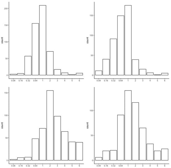
Figure 1. Histograms of selected $\lambda$ in Cases 1 (top) and 2 (bottom) via BIC (left) and AIC (right).

6. Real Data Applications

In this section, we use the regularized BEKK representation to study the volatility spillover effect and find optimal Markowitz’s mean–variance portfolios. The data we studied consist of daily log-returns of 18 stocks during the period 4 January 2016–31 January 2018, which are listed in Table 3 (NASDAQ Stock Symbols n.d.). Figure 2 shows the time series of these 18 stocks and Table 4 summarizes the sample mean, the sample standard deviation, the sample skewness, the sample kurtosis, and the correlations of these 18 series. All the correlations are positive for every two stocks in the selected period, and, except for IPG, all the stocks have a positive mean. The sample kurtosis for some stocks is way larger than 3, which indicates that we cannot simply assume that those returns are following normal distributions individually. Hence, it is natural to employ a suitable time series model to examine the data.

Table 3. Full names of 18 tickers.

Ticker	Company	Ticker	Company
GOOG	Alphabet Inc., Mountain View, CA, USA	GWW	W.W. Grainger, Inc., Lake Forest, FL, USA
IBM	International Business Machines Corporation, Armonk, NY, USA	JPM	JPMorgan Chase & Co., New York, NY, USA
MSFT	Microsoft Corporation, Redmond, WA, USA	NKE	Nike Inc., Beaverton, OR, USA
ORCL	Oracle Corporation, Austin, TX, USA	TIF	Tiffany & Co., New York, NY, USA
IPG	The Interpublic Group of Companies, New York, NY, USA	MAS	Masco Corporation, Livonia, MI, USA
MCD	Mcdonald’s Corp., Chicago, IL, USA	NFLX	Netflix, Inc., Los Gatos, CA, USA
RL	Ralph Lauren Corporation, New York, NY, USA	TXT	Textron Inc., Providence, RI, USA
LNC	Lincoln National Corporation, Radnor, PA, USA	MRO	Marathon Oil Corporation, Houston, TX, USA
TGT	Target Corporation, Minneapolis, MN, USA	WMT	Walmart Inc., Bentonville, AR, USA

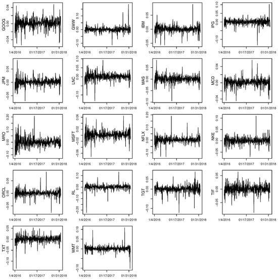
Figure 2. Daily returns of 18 stocks from 4 January 2016 to 31 January 2018.

Table 4. Correlation and statistical features of 18 stocks for 2016–2017.

	GOOG	GWW	IBM	JPM	MSFT	NKE	ORCL	TIF	IPG	MAS	MCD	NFLX	RL	TXT	LNC	MRO	TGT	WMT
Mean	7.037 × ${10}^4$	5.164 × ${10}^4$	4.297 × ${10}^4$	1.150 × ${10}^3$	1.033 × ${10}^3$	1.420 × ${10}^4$	6.439 × ${10}^4$	8.143 × ${10}^4$	−7.648 × ${10}^5$	1.029 × ${10}^3$	8.891 × ${10}^4$	1.304 × ${10}^3$	1.610 × ${10}^4$	7.103 × ${10}^4$	1.148 × ${10}^3$	1.217 × ${10}^3$	5.523 × ${10}^5$	1.116 × ${10}^3$
Std. Dev.	0.013	0.016	0.011	0.013	0.012	0.014	0.012	0.015	0.015	0.014	0.009	0.023	0.021	0.015	0.019	0.034	0.017	0.012
Skewness	−0.440	0.124	0.291	0.348	0.040	0.509	0.097	−0.391	−1.779	−0.456	0.005	0.635	−2.332	−1.438	−0.779	0.640	−1.108	2.291
Kurtosis	6.120	16.399	14.446	8.907	8.926	11.683	15.022	6.274	16.842	9.409	9.640	17.196	33.455	17.970	10.830	7.383	13.600	24.910
GOOG		0.04	0.24	0.26	0.67	0.28	0.36	0.22	0.28	0.33	0.29	0.44	0.15	0.23	0.27	0.11	0.06	0.13
GWW			0.38	0.34	0.13	0.17	0.16	0.24	0.29	0.27	0.03	0.06	0.09	0.34	0.28	0.21	0.16	0.09
IBM				0.38	0.30	0.15	0.42	0.27	0.30	0.31	0.12	0.13	0.15	0.39	0.37	0.19	0.15	0.14
JPM					0.37	0.23	0.38	0.41	0.31	0.44	0.23	0.19	0.28	0.52	0.78	0.36	0.16	0.09
MSFT						0.26	0.45	0.29	0.29	0.38	0.35	0.36	0.19	0.32	0.33	0.20	0.08	0.12
NKE							0.20	0.23	0.30	0.30	0.18	0.18	0.33	0.23	0.30	0.12	0.27	0.16
ORCL								0.34	0.26	0.36	0.26	0.26	0.15	0.30	0.35	0.19	0.09	0.12
TIF									0.23	0.33	0.14	0.18	0.25	0.33	0.42	0.26	0.27	0.11
IPG										0.38	0.09	0.12	0.21	0.26	0.32	0.15	0.21	0.10
MAS											0.28	0.23	0.26	0.36	0.46	0.20	0.24	0.12
MCD												0.14	0.13	0.12	0.16	0.07	0.09	0.16
NFLX													0.10	0.22	0.19	0.07	0.02	0.09
RL														0.22	0.35	0.16	0.31	0.09
TXT															0.53	0.26	0.17	0.09
LNC																0.39	0.19	0.05
MRO																	0.08	0.04
TGT																		0.36

6.1. Volatility Spillovers

To use the MGARCH–BEKK representation to analyze the market, consisting of 18 stocks, we should realize that certain types of regularization or shrinkage are necessary, due to the complexity of the volatility dynamics. In particular, we use the proposed $L_1$-regularized BEKK(1,1) model and procedure to study the volatility spillover among the 18 stocks. We first compute the PQML estimates of the model for different $\lambda$s. Figure 3 shows the estimated structures of estimated coefficient matrices ${\widehat{A}}_{\lambda }$ and ${\widehat{B}}_{\lambda }$ for $\lambda =4,2,1,0.5,0.3$, in which the nonzero values of ${\widehat{A}}_{\lambda }$ and ${\widehat{B}}_{\lambda }$ are represented as the directional lines among stocks. Since matrices A and B in the model are not symmetric before the quadratic forms, we use the directional lines to distinguish the nonzero elements between upper-diagonal and lower-diagonal elements. Specifically, if $a_{ij}\ne 0$, the directional line progresses from i to j. As the PQML estimates ${\widehat{A}}_{\lambda }$ and ${\widehat{B}}_{\lambda }$ tell us the significant interdependence and contagion effects of the 18 stocks, the network structures in Figure 3 provide a clear representation on volatility spillover. Furthermore, we notice that, for some moderate values of $\lambda$, for example, $\lambda =0.5$, ${\widehat{A}}_{\lambda }$ is very sparse, whereas ${\widehat{B}}_{\lambda }$ demonstrates more interdependence among stocks. When larger values of $\lambda$ are used in the regularization procedure, the PQML estimates ${\widehat{A}}_{\lambda }$ are quickly shrunk into diagonal matrices, and ${\widehat{B}}_{\lambda }$ also become more sparse than for the case $\lambda =0.5$.

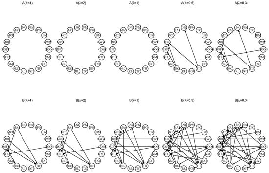
Figure 3. The network structure of estimated matrices A (top) and B (bottom) under different $\lambda$s.

Using the PQML estimates of ${\widehat{A}}_{\lambda }$, ${\widehat{B}}_{\lambda }$, and ${\widehat{C}}_{\lambda }$ and the BEKK(1, 1) representation, we compute the estimated volatilities and the dynamic correlations among 18 stocks. Figure 4 shows the volatilities estimated by the regularized BEKK(1,1) model with $\lambda =2,0.5$ and univariate GARCH models. Note that most volatility series estimated by the three models are similar, except for stocks NFLX, ORCL, and TIF. We also show the estimated dynamic correlations among 18 stocks in a regularized BEKK(1,1) model with $\lambda =1$ in Figure 5. We note that most correlations among the 18 stocks are positive during the sample period.

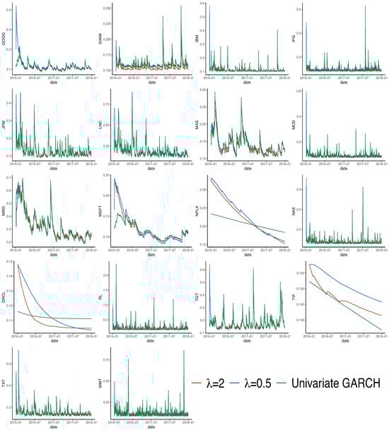
Figure 4. Estimated volatilities by regularized BEKK(1,1) with $\lambda =2$ (red lines), $\lambda =0.5$ (blue lines), and univariate GARCH models (green lines).

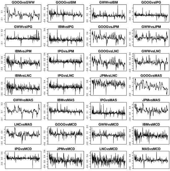
Figure 5. Daily estimated conditional correlations when $\lambda =1$.

To show the overall volatility spillover, we extend the idea of the spillover index in Diebold and Yilmaz (2009). Specifically, note that $E\left[{ϵ}_{t+1}{ϵ}_{t+1}^{\prime }\right]={\Sigma }_{t+1}={\Sigma }_{t+1}^{\frac{1}{2}}{\left({\Sigma }_{t+1}^{\frac{1}{2}}\right)}^{\prime }$, where ${\Sigma }_{t+1}^{\frac{1}{2}}$ is the unique lower-triangular Cholesky factor of ${\Sigma }_{t+1}$. We denote elements of ${\Sigma }_t^{\frac{1}{2}}$ by ${\sigma }_{\frac{1}{2},i,j,t}$; then, the Spillover Index $S_{t+1}$ is defined as

$$S_{t+1}=\frac{{\sum }_{i,j=1,i\ne j}^n{\widehat{\sigma }}_{\frac{1}{2},i,j,t+1}^2}{trace\left({\widehat{\Sigma }}_{t+1}\right)}\times 100\%,$$

where n is the number of stocks, which is equal to 18. We plot the daily spillover indices of 18 stocks for $\lambda =2$ and $0.5$. The spillover indices during the sample period vary between 5% and 80%, and smaller $\lambda$s seem to generate more correlations among stocks. In particular, three big spikes can be found on 4 February 2016, 24 June 2016, and 9 November 2016. In addition to finding the PQML estimates for different $\lambda$s, we also find the whole ${Ł}_1$ regularization path. Note that the number of parameters in the BEKK(1,1) model for 18 stocks is $p=819$, and we only show the regularized path for $819-18\times 3=765$ off-diagonal elements in ${\widehat{A}}_{\lambda }$, ${\widehat{B}}_{\lambda }$, and ${\widehat{C}}_{\lambda }$. And both plots are shown in Figure 6.

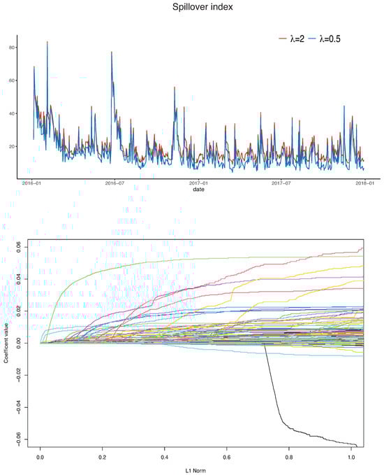
Figure 6. Daily spillover index (top) and regularization paths of estimated off-diagonal parameters in BEKK regularization Model represented by different colors (bottom).

6.2. Portfolio Optimization

We further apply the regularized BEKK model to Markowitz mean–variance portfolio optimization (Markowitz 1952). Using portfolio variance as a measure of the risk, Markowitz portfolio optimization theory provides an optimal pay-off between the profit and the risk. Since the means and covariance matrix of assets are assumed to be known in the theory, they need to be estimated before being plugged into the framework. For high-dimensional portfolios, regularized methods are commonly used to achieve better performance. For instance, Brodie et al. (2009) and Fastrich et al. (2015) used an $L_1$ penalty function for sparse portfolios, and Di Lorenzo et al. (2012) used a concave optimization-based approach to estimate the optimal portfolio. In our case, we use the regularized BEKK model to predict the covariance matrices in the next period, and then apply Markowitz portfolio theory to find the optimal portfolios.

In particular, we assume that the portfolio consists of $n=18$ risky assets and denote ${\mu }_t$ and ${\Sigma }_t$ as the mean and covariance matrix, respectively, of the n risk assets at time t. Let $\mathbf{1}={(1,\cdots ,1)}^{\prime }$ be an n-dimensional vector of ones. Markowtiz mean–variance portfolio theory minimizes the variance of the portfolio ${min}_{w_t}{w}_t^{\prime }{\Sigma }_t{w}_t$, subject to the constraint $w_t^{\prime }\mathbf{1}=1$ and $w_t^{\prime }{\mu }_t={\mu }_{*}$, where ${\mu }_{*}$ is the target return. When short selling is allowed, the efficient portfolio can be explicitly expressed as

$$w_{\mathrm{effi},t}=\frac{\tilde{b}}{\tilde{d}}{\Sigma }_t^{-1}\mathbf{1}-\frac{\tilde{a}}{\tilde{d}}{\Sigma }_t^{-1}{\mu }_t+{\mu }_{*}\left(\frac{\tilde{c}}{\tilde{d}}{\Sigma }_t^{-1}{\mu }_t-\frac{\tilde{a}}{\tilde{d}}{\Sigma }_t^{-1}\mathbf{1}\right),$$

where $\tilde{a}={\mu }_t{\Sigma }_t^{-1}\mathbf{1}$, $\tilde{b}={\mu }_t^{\prime }{\Sigma }_t{\mu }_t$, $\tilde{c}={\mathbf{1}}^{\prime }{\Sigma }_t\mathbf{1}$, and $\tilde{d}=\tilde{b}\tilde{c}-{\tilde{a}}^2$. When the target return ${\mu }_{*}$ is chosen to minimize the variance of the efficient portfolio, we obtain the global minimum variance (GMV) portfolio:

$$w_{\mathrm{minvar},t}={\Sigma }_t^{-1}\mathbf{1}/\left({\mathbf{1}}^{\prime }{\Sigma }_t\mathbf{1}\right).$$

For comparison purposes, we also use another three multivariate volatility models to predict the covariance matrices of $n=18$ stocks. The first is very simple, and it assumes a constant covariance matrix for n stocks. The second is a factor-GARCH model (Alexander 2000; Engle 1990; van der Weide 2002; Vrontos et al. 2003), which assumes the following for asset return vector $r_t$, factors $f_t$, and volatilties of k independent factors:

$$r_t=W{f}_t,\mathrm{Cov}\left(f_t\right)={\Sigma }_t=\mathrm{diag}\{{\sigma }_{1t}^2,{\sigma }_{2t}^2,\dots ,{\sigma }_{kt}^2\},$$

$${\sigma }_{it}^2=1+{\beta }_i{x}_{i,t-1}^2+{\gamma }_i{\sigma }_{i,t-1}^2,$$

where W is a $k\times k$ lower-triangular matrix with diagonal elements equal to 1 and $x_t={(x_{1t},\dots ,x_{kt})}^{\prime }$ is a vector of k independent factors. The third covariance model is a dynamic conditional correlation GARCH (DCC–GARCH) model (Engle 2002), which has the form

$$r_t={\Sigma }_t^{\frac{1}{2}}{ϵ}_t,{ϵ}_t\sim N(0,I_n),{\Sigma }_t=D_t{R}_t{D}_t,$$

$$Q_t=(1-\alpha -\beta )C+\alpha s_{t-1}{s}_{t-1}^{\prime }+\beta Q_{t-1,}{R}_t=\mathrm{diag}{\left(Q_t\right)}^{-\frac{1}{2}}{Q}_t\mathrm{diag}{\left(Q_t\right)}^{-\frac{1}{2}},$$

where $D_t=\mathrm{diag}(d_{1t},\cdots ,d_{nt})$, $s_{i,t}=r_{i,t}/d_{i,t}$, $s_t={(s_{1,t},\cdots ,s_{T,t})}^{\prime }$, and $R_t$ is the conditional correlation matrix at time t, that is, $R_t=\mathrm{Corr}\left(r_t\right|{\mathcal{F}}_{t-1})$. And C is the unconditional correlation matrix, i.e., $C=E\left(R_t\right)$. The matrix $Q_t$ can be interpreted as a conditional covariance matrix of devolatilized residuals. For the dynamics of the univariate volatilities, $d_{i,t}$s are assumed to follow a GARCH(1,1) process:

$$d_{i,t}={\omega }_i+a_i{r}_{i,t-1}^2+b_i{d}_{i,t-1}^2,$$

where $(w_i,a_i,b_i)$ are GARCH(1,1) parameters.

Let $t=$ 2 January 2018, ⋯, 31 January 2018; we first fit 4 covariance models to the returns of 18 stocks from 4 January 2016 to t, and then compute the 1-day-ahead prediction of covariance matrices. Using the predicted covariance matrices, we compute the efficient portfolios $w_{\mathrm{minvar},t+1}$ and $w_{\mathrm{effi},t+1}$ for ${\mu }_{*}=0.15\%,0.10\%$, and $0.05\%$. Table 5 shows the means, standard deviations (SD), and the information ratios (IR, i.e., ratio of means and standard deviations) for realized portfolio returns in the month of January 2018. As argued by Engle and Colacito (2006) and Engle et al. (2019), these statistics are good measurements of the out-of-sample performance of Markowitz portfolios. As DeMiguel et al. (2007) claimed that it is difficult to outperform equally weighted portfolios in terms of the out-of-sample mean for Markowitz portfolios, we also include the performance of equally weighted portfolios as a benchmark in Table 5. We note that all the means generated from four covariance models are smaller than that from equally weighted portfolios (0.430%), and the standard deviations of covariance models, except the factor GARCH, are smaller than that of equally weighted portfolios. Notably, the regularized BEKK model consistently maintains the second-best mean performances at 0.39%, 0.352%, 0.382%, and 0.416% for GMV, and ${\mu }_{*}$ values of 0.15%, 0.10%, and 0.05%. However, the information ratio of the regularized BEKK model surpasses that of all other portfolios. It achieves the highest values across all scenarios—0.601, 0.540, 0.654, and 0.657—for GMV and ${\mu }_{*}=0.15\%,0.10\%$, and $0.05\%$. These results show the robustness and efficiency of the regularized BEKK model in portfolio optimization, consistently delivering competitive mean performance and superior risk-adjusted returns compared to other covariance models.

Table 5. Performance of portfolios using different covariance models.

Model	Mean (%)	SD. (%)	IR	Mean (%)	SD. (%)	IR
Equally weighted	0.430	0.761	0.565
	GMV			${\mu }_{*}=0.15\%$
Regularized BEKK	0.390	0.650	0.601	0.352	0.652	0.540
Factor GARCH	0.326	0.885	0.368	0.223	1.200	0.186
DCC–GARCH	0.244	0.665	0.367	0.302	0.677	0.446
Constant covariance	0.261	0.658	0.397	0.165	0.777	0.212
	${\mu }_{*}=0.10\%$			${\mu }_{*}=0.05\%$
Regularized BEKK	0.382	0.585	0.654	0.416	0.633	0.657
Factor GARCH	0.210	1.169	0.180	0.221	1.321	0.167
DCC–GARCH	0.286	0.631	0.452	0.316	0.660	0.479
Constant covariance	0.219	0.669	0.327	0.273	0.668	0.409

7. Discussion and Conclusive Remarks

Modeling the dynamics of high-dimensional covariance matrices is an interesting and challenging problem in both financial econometrics and high-dimensional time series analysis. To address this issue, this paper proposes an inference procedure with $L_1$ regularization for the sparse representation of high-dimensional BEKK and to obtain a class of penalized quasi-maximum likelihood estimators. The proposed regularization allows us to find significant parameters in the BEKK representation and shrink the non-essential ones to zero, hence providing a sparse estimate of the BEKK representations. We show that the sparse BEKK representation has suitable theoretical properties and is promising for applications in portfolio optimization and volatility spillover.

The proposed sparse BEKK representation also contributes to the application of machine learning methods in time series modeling. As most discussion on applying regularization methods to time series modeling focuses on regularizing high-dimensional vector autoregressive models and their variants (Nicholson et al. 2017; Sánchez García and Cruz Rambaud 2022), it seems that the sparse representation of dynamics of high-dimensional variance–covariance matrices has been ignored in the literature. While obtaining a sparse representation of the dynamics within high-dimensional variance–covariance matrices is crucial to enhance interpretability in time series modeling, our study bridges this gap by considering a basic $L_1$ regularization method. One obvious extension from our current study is to replace the $L_1$ penalty with other types of penalty for high-dimensional MGARCH models, for instance, the SCAD penalty (Fan and Li 2001), the adaptive LASSO (Zou 2006), and the group LASSO (Yuan and Lin 2006). With different types of penalty functions, one can regularize the assets in the model with different requirements, hence causing the estimates to have different kinds of asymptotic properties.

As the proposed sparse BEKK representation simplifies the dynamics of covariance matrices of high-dimensional time series, it has advantages over existing MGARCH models in some financial applications. In particular, the sparse BEKK representation can capture significant volatility spillover effects in high-dimensional financial time series, which usually cannot be analyzed using other MGARCH models. Since significant volatility spillover is captured, the proposed method also improves the performance of portfolio optimization based on the dynamics of high-dimensional covariance matrices. The proposed procedure can certainly be extended to incorporate more empirical aspects of financial time series. Taking the leverage effect as an example, one may modify the regularization procedure to obtain sparse representation of high-dimensional multivariate exponential or threshold GARCH models.

Although the proposed framework shows advantages in modeling dynamics of high-dimensional covariance matrices, the computational challenge is not completely resolved. The main reason is that the proposed inference procedure involves a step of computing derivatives via the Kronecker product of parameter matrices. Since the Kronecker product turns two $n\times n$ matrices into an $n^2\times n^2$ matrix, the requirement for computational memory resources increases significantly. Hence, the proposed procedure is suitable for problems in which the number of component time series ranges from several to 100. If the number of assets progresses beyond 200, the computational cost is still a major concern. One possible remedy for this is training a neural network to approximate the regularized likelihood of the high-dimensional model. In such a way, the proposed regularization using the high-dimensional MGARCH model can be extended to characterize the dynamics of covariance matrices of larger size.

Appendix A.1. Proof of Propostion 2

Let ${\mathfrak{R}}_t$,$\mathfrak{C}$, and ${\Sigma }_t^{*}$ be defined by

$${\mathfrak{R}}_t={(vech{\left(r_t{r}_t^{\prime }\right)}^{\prime },\dots ,vech{\left(r_{t-m+1}{r}_{t-m+1}^{\prime }\right)}^{\prime })}^{\prime },{\Sigma }_t^{*}={(vech{\left({\Sigma }_t\right)}^{\prime },\dots ,vech{\left({\Sigma }_{t-m+1}\right)}^{\prime })}^{\prime },$$

where $m=max(a,b)$, and let

$$\mathfrak{C}={(vech{\left(C^{\prime }C\right)}^{\prime },0,\dots ,0)}^{\prime },$$

with dimensions $mn(n+1)/2$.

Define $A=\left(\begin{array}{ccccc}{\tilde{A}}_1& \dots & \dots & \dots & {\tilde{A}}_m\\ I& 0& 0& \cdots & 0\\ 0& \ddots & \ddots & \ddots & ⋮\\ ⋮& \ddots & \ddots & \ddots & 0\\ 0& \dots & 0& I& 0\end{array}\right)$ and $B=\left(\begin{array}{ccccc}{\tilde{B}}_1& \dots & \dots & \dots & {\tilde{B}}_m\\ I& 0& 0& \cdots & 0\\ 0& \ddots & \ddots & \ddots & ⋮\\ ⋮& \ddots & \ddots & \ddots & 0\\ 0& \dots & 0& I& 0\end{array}\right),$ with convention ${\tilde{A}}_i=0$ if $i>a$ and ${\tilde{B}}_i=0$ if $i>b.$ Then, the model can be written as

$${\Sigma }_t^{*}=\mathfrak{C}+A{\mathfrak{R}}_t+B{\Sigma }_{t-1}^{*}=\sum _{k=0}^{t-1}\left[B^k\left(\theta \right)\mathfrak{C}\left(\theta \right)\right]+B^t\left(\theta \right){\Sigma }_0^{*}+\sum _{k=0}^{t-1}{B}^k\left(\theta \right)A\left(\theta \right)L^k{\mathfrak{R}}_{t-1}\left({\theta }_0\right)$$

where L is the backshift operator $L{r}_t=r_{t-1}$. Here, ${\Sigma }_0^{*}$ is fixed and ${\mathfrak{R}}_{\mathfrak{t}}$ depends on ${\theta }_0$ but is not a function of $\theta$. Then, we have

$$\frac{\partial {\Sigma }_t^{*}}{\partial {\theta }_i}=\frac{\partial }{\partial {\theta }_i}\left(\sum _{k=0}^{t-1}{\tilde{B}}^k\mathfrak{C}\right)+\frac{\partial }{\partial {\theta }_i}\left({\tilde{B}}^t\right){\Sigma }_0^{*}+\frac{\partial }{\partial {\theta }_i}\left(\sum _{k=0}^{t-1}{\tilde{B}}^k\tilde{A}L\right){\mathfrak{R}}_{t-1}$$

(A1)

Since

$$\frac{\partial {\tilde{B}}^k}{\partial \theta }=\sum _{j=0}^{k-1}{\tilde{B}}^j\frac{\partial \tilde{B}}{\partial {\theta }_j}{\tilde{B}}^{k-1-j},$$

we have

$$∥B^j\frac{\partial B}{\partial {\theta }_j}{B}^{k-1-j}∥\le \left|\right|B^j\left|\right|∥\frac{\partial B}{\partial {\theta }_i}∥\left|\right|B^{k-1-j}\left|\right|,j=0,\cdots ,k-1.$$

Applying Lemma A.3. from Comte and Lieberman (2003), $\left|\right|B^k\left|\right|\le \Psi k^{n_0}{\rho }_0^k$ for all k, we have

$$∥B^j\frac{\partial B}{\partial {\theta }_j}{B}^{k-1-j}∥\le {\Psi }^2{k}^{n_0}{\rho }_0^k∥\frac{\partial B}{\partial {\theta }_i}∥.$$

in which $n_0$ is a fixed number, $\Psi$ is a constant independent of $\theta$, and $-1<{\rho }_0<1$.

To bound (A1), there are three terms to bound:

$$\begin{array}{ccc}& & ∥\frac{\partial }{\partial {\theta }_i}\left(\sum _{k=0}^{t-1}{\tilde{B}}^k\mathfrak{C}\right)∥=∥\sum _{k=1}^{t-1}\frac{\partial {\tilde{B}}^k}{\partial {\theta }_i}\mathfrak{C}+\sum _{k=0}^{t-1}{\tilde{B}}^k\frac{\partial \mathfrak{C}}{\partial {\theta }_i}∥\le \hfill \\ & & \sum _{k=1}^{t-1}∥\frac{\partial {\tilde{B}}^k}{\partial {\theta }_i}∥\left|\right|\left|\mathfrak{C}\right||+\sum _{k=0}^{t-1}\left|\right|{\tilde{B}}^k\left|\right|∥\frac{\partial \mathfrak{C}}{\partial {\theta }_i}∥\hfill \\ & & \le {\Psi }^2\left|\right|\mathfrak{C}\left|\right|\sum _{k=1}^{t-1}{k}^{n_0}{\rho }_0^k∥\frac{\partial \tilde{B}}{\partial {\theta }_i}∥+\Psi ∥\frac{\partial \mathfrak{C}}{\partial {\theta }_i}∥\sum _{k=0}^{t-1}{k}^{n_0}{\rho }_0^k\hfill \\ & & \le \pi \left(n_0\right)\Psi (\Psi |\left|\mathfrak{C}\right||·∥\frac{\partial \tilde{B}}{\partial {\theta }_i}∥+∥\frac{\partial \mathfrak{C}}{\partial {\theta }_i}∥),\hfill \end{array}$$

using ${\sum }_{k=0}^{t-1}{k}^{n_0}{\rho }_0^k\le {\sum }_{k=0}^t{k}^{n_0}{\rho }_0^{k-1}\le {\sum }_{k=0}^{\infty }{k}^{n_0}{\rho }_0^{k-1}=\pi \left(n_0\right)$, where $\pi \left(n_0\right)$ is a constant that only depends on $n_0.$ And, if ${\rho }_0=0,$ this term is then easily bounded because $\tilde{B}$ is the nilpotent and all sums are finite. In the same way,

$$∥\frac{\partial }{\partial {\theta }_i}\left({\tilde{B}}^t\right){\Sigma }_0^{*}∥\le \Psi \pi \left(n_0\right)∥\frac{\partial \tilde{B}}{\partial {\theta }_i}∥\left|\right|{\Sigma }_0^{*}\left|\right|.$$

Finally,

$$\left|\right|\frac{\partial }{\partial {\theta }_i}\left(\sum _{k=0}^{t-1}{\tilde{B}}^k{L}^k\tilde{A}\right){\mathfrak{R}}_{t-1}\left|\right|\le \left|\right|\sum _{k=0}^{t-1}(\frac{\partial }{\partial {\theta }_i}{\tilde{B}}^k{L}^k\widetilde{A)}{\mathfrak{R}}_{t-1}\left|\right|+\left|\right|[\sum _{k=0}^{t-1}{\tilde{B}}^k{L}^k\left(\frac{\partial }{\partial {\theta }_i}\tilde{A}\right){\mathfrak{R}}_{t-1}\left|\right|.$$

Denote the first and second sums on the right-hand side of the inequality as $T_1$ and $T_2$, respectively, we have

$$\begin{array}{ccc}& & \left|\right|T_1\left|\right|\le {\Psi }^2\left(\sum _{k=1}^{t-1}{k}^{n_0+1}{\rho }_0^{k-1}\left|\right|\tilde{A}\left|\right|·\left|\right|{\mathfrak{R}}_{t-k-1}\left|\right|\right)·\left|\right|\frac{\partial \tilde{B}}{\partial {\theta }_i}\left|\right|\hfill \\ & & \le {\Psi }^2\left|\right|\tilde{A}\left|\right|·\left|\right|\frac{\partial \tilde{B}}{\partial {\theta }_i}\left|\right|·\left(\sum _{k=1}^{t-1}{k}^{n_0+1}{\rho }_0^{k-1}\right)·\underset{t}{sup}\left|\right|{\mathfrak{R}}_{\mathfrak{t}}\left|\right|\le \pi (n_0+1){\Psi }^2\left|\right|\tilde{A}\left|\right|·\left|\right|\frac{\partial \tilde{B}}{\partial {\theta }_i}\left|\right|·\underset{t}{sup}\left|\right|{\mathfrak{R}}_t\left|\right|,\hfill \end{array}$$

and

$$\left|\right|T_2\left|\right|\le {\Psi }^2\pi \left(n_0\right)\left|\right|\frac{\partial \tilde{A}}{\partial {\theta }_i}\left|\right|\underset{t}{sup}\left|\right|{\mathfrak{R}}_t\left|\right|.$$

By our assumption, $\left|\right|\mathfrak{C}\left|\right|,\left|\right|\frac{\partial \mathfrak{C}}{\partial {\theta }_i}\left|\right|,\left|\right|\tilde{A}\left|\right|,\left|\right|\frac{\partial \tilde{A}}{\partial {\theta }_i}\left|\right|,\left|\right|\frac{\partial \tilde{B}}{\partial {\theta }_i}\left|\right|,\left|\right|{\Sigma }_0^{*}\left|\right|$ are all bounded. And there exists a constant w such that $\left|\right|\frac{\partial {\Sigma }_t^{*}}{\partial {\theta }_i}\left|\right|=m\left|\right|\frac{\partial {\Sigma }_t}{\partial {\theta }_i}\left|\right|.$ Hence,

$$\left|\right|\frac{\partial {\Sigma }_t}{\partial {\theta }_i}\left|\right|\le {\Psi }_1+{\Psi }_2\underset{t}{sup}\left|\right|{\mathfrak{R}}_t\left|\right|.$$

where ${\Psi }_1=\Psi \pi \left(n_0\right)(\Psi |\left|\mathfrak{C}\right||·\left|\right|\frac{\partial \tilde{B}}{\partial {\theta }_i}\left|\right|+\left|\right|\frac{\partial \mathfrak{C}}{\partial {\theta }_i}\left|\right|)+\Psi \pi \left(n_0\right)\left|\right|\frac{\partial \tilde{B}}{\partial {\theta }_i}\left|\right|·\left|\right|{\Sigma }_0^{*}\left|\right|$, and ${\Psi }_2={\Psi }^2\pi (n_0+1)\left|\right|\tilde{A}\left|\right|·\left|\right|\frac{\partial \tilde{B}}{\partial {\theta }_i}\left|\right|+{\Psi }^2\pi \left(n_0\right)\left|\right|\frac{\partial \tilde{A}}{\partial {\theta }_i}\left|\right|$. □

Appendix A.2. Proof of Proposition 4

As $\frac{\partial l_t\left(\theta \right)}{\partial {\theta }_i}=Tr(\frac{\partial {\Sigma }_t}{\partial {\theta }_i}{\Sigma }_t^{-1}-r_t{r}_t^{\prime }{\Sigma }_t^{-1}\frac{\partial {\Sigma }_t}{\partial {\theta }_i}{\Sigma }_t^{-1})$, where $Tr(·)$ denote the trace of a matrix, and $E\left[r_t{r}_t^{\prime }\right|{\mathcal{F}}_{t-1}]={\Sigma }_t$, we, hence, have $E\left[\frac{\partial l_t\left(\theta \right)}{\partial {\theta }_i}\right|{\mathcal{F}}_{t-1}]=0,$ which means that $\frac{\partial l_t\left(\theta \right)}{\partial {\theta }_i}$ is a martingale difference. Then, we want to prove that $E\left[\right|T^{1/2}{T}^{-1}{\sum }_{t=1}T\frac{\partial l_t\left({\theta }^0\right)}{\partial {\theta }_i}{|}^m]=E[|T^{-1/2}{\sum }_{t=1}^T\frac{\partial l_t\left({\theta }^0\right)}{\partial {\theta }_i}{|}^m]<\infty$ holds for $m=4$. By Lemma 2, this proof is thus completed if we show that $E\left[\right|\frac{\partial l_t\left({\theta }^0\right)}{\partial {\theta }_i}{|}^4]<\infty .$ By Proposition 2, $∥\frac{\partial {\Sigma }_t}{\partial {\theta }_i}∥\le {\Psi }_1+{\Psi }_{2}sup\left|\right|vech\left(r_t{r}_t^{\prime }\right)\left|\right|$. Since

$$\begin{array}{ccc}& & ∥\frac{\partial {\Sigma }_t}{\partial {\theta }_i}{\Sigma }_t^{-1}-r_t{r}_t^{\prime }{\Sigma }_t^{-1}\frac{\partial {\Sigma }_t}{\partial {\theta }_i}{\Sigma }_t^{-1}∥=∥(I-r_t{r}_t^{\prime }{\Sigma }_t^{-1})\frac{\partial {\Sigma }_t}{\partial {\theta }_i}{\Sigma }_t^{-1}∥\hfill \\ & & \le \left|\right|(I-r_t{r}_t^{\prime }{\Sigma }_t^{-1})\left|\right|∥\frac{\partial {\Sigma }_t}{\partial {\theta }_i}{\Sigma }_t^{-1}∥\le \left|\right|(I-r_t{r}_t^{\prime }{\Sigma }_t^{-1})\left|\right|∥\frac{\partial {\Sigma }_t}{\partial {\theta }_i}∥\left|\right|{\Sigma }_t^{-1}\left|\right|,\hfill \end{array}$$

it is equivalent to show that

$$E\left[{\left|\frac{\partial l_t\left({\theta }^0\right)}{\partial {\theta }_i}\right|}^4\right]=E\left[T{r}^4\left(\frac{\partial {\Sigma }_t}{\partial {\theta }_i}{\Sigma }_t^{-1}-r_t{r}_t^{\prime }{\Sigma }_t^{-1}\frac{\partial {\Sigma }_t}{\partial {\theta }_i}{\Sigma }_t^{-1}\right)\right]<\infty .$$

Since $Tr\left(AB\right)\le \left|\right|A\left|\right|·\left|\right|B\left|\right|$ and $\left|\right|{\Sigma }_t^{-1}\left|\right|$ is finite, there exists a constant M such that $\left|\right|{\Sigma }_t^{-1}\left|\right|\le M$ for all t. Additionally, $\left|\right|(I-r_t{r}_t^{\prime }{\Sigma }_t^{-1})\left|\right|\le \left|\right|I\left|\right|+\left|\right|r_t{r}_t^{\prime }\left|\right|·\left|\right|{\Sigma }_t{\left|\right|}^{-1}\le 1+M\left|\right|r_t{r}_t^{\prime }\left|\right|$, then

$$Tr\left(\frac{\partial {\Sigma }_t}{\partial {\theta }_i}{\Sigma }_t^{-1}-r_t{r}_t^{\prime }{\Sigma }_t^{-1}\frac{\partial {\Sigma }_t}{\partial {\theta }_i}{\Sigma }_t^{-1}\right)\le \left|\right|(I-r_t{r}_t^{\prime }{\Sigma }_t^{-1})\left|\right|\left|\right|{\Sigma }_t^{-1}\left|\right|∥\frac{\partial {\Sigma }_t}{\partial {\theta }_i}∥$$

$$E\left[T{r}^4\left(\frac{\partial {\Sigma }_t}{\partial {\theta }_i}{\Sigma }_t^{-1}-r_t{r}_t^{\prime }{\Sigma }_t^{-1}\frac{\partial {\Sigma }_t}{\partial {\theta }_i}{\Sigma }_t^{-1}\right)\right]\le E\left[\right(1+Msup\left|\right|r_t{r}_t^{\prime }{\left|\right|)}^4({\Psi }_1+{\Psi }_2\underset{t}{sup}\left|\right|vech\left(r_t{r}_t^{\prime }\right)\left|\right|{)}^4].$$

Because $\left|\right|A\left|\right|\le \left|\right|vech\left(A\right)\left|\right|\le rank\left(A\right)\left|\right|A\left|\right|$, there exists a constant k such that $\left|\right|r_t{r}_t^{\prime }\left|\right|=k\left|\right|vech\left(r_t{r}_t^{\prime }\right)\left|\right|$. Hence, if we let $\left|\right|vech\left(r_t{r}_t^{\prime }\right)\left|\right|=\left|\right|{\mathfrak{R}}_t\left|\right|,$

$$\begin{array}{ccc}& & E\left[\right(1+M\underset{t}{sup}\left|\right|r_t{r}_t^{\prime }{\left|\right|)}^4({\Psi }_1+{\Psi }_2\underset{t}{sup}\left|\right|{\mathfrak{R}}_t\left|\right|{)}^4]\hfill \\ & =& E\left[\right(1+kM\underset{t}{sup}\left|\right|{\mathfrak{R}}_t{\left|\right|)}^4({\Psi }_1+{\Psi }_2\underset{t}{sup}\left|\right|{\mathfrak{R}}_t\left|\right|{)}^4]=E(\sum _{i=0}^8{a}_i\left|\right|{\mathfrak{R}}_t{\left|\right|}^i)\hfill \end{array}$$

where $a_{i}s$ are constants. Since $r_t\sim {\Sigma }_t^{\frac{1}{2}}{ϵ}_t$, where ${ϵ}_{t}s$ follow a normal distribution, $r_{t}s$, hence, admit 16 moments of order. Hence, $E\left|\right|{\mathfrak{R}}_t{\left|\right|}^i<\infty ,$ for i from 0 to 8. Hence, $E\left({\sum }_{i=0}^8{a}_i\right|\left|{\mathfrak{R}}_t\right|{|}^i)<\infty$; then, $E\left[\right|\frac{\partial l_t\left({\theta }^0\right)}{\partial {\theta }_i}{|}^4]<\infty$.

Next, we check (c) and (d). (c) is clear, as we said before. By (III) in Lemma 1, the derivative of $H_{{\mathcal{U}}_0,T}\left(\theta \right)$ is bounded. By the mean-value theorem,

$$vec(H_{{\mathcal{U}}_0,T}({\theta }^{\left(1\right)},0)-H_{{\mathcal{U}}_0,T}({\theta }^{\left(2\right)},0))=\frac{\partial H_{{\mathcal{U}}_0,T}(\theta ,0)}{\partial \theta }{|}_{\theta ={\theta }^{*}}·({\theta }^{\left(1\right)}-{\theta }^{\left(2\right)}).$$

Hence,

$$\begin{array}{ccc}& & \left|\right|H_{{\mathcal{U}}_0,T}({\theta }^{\left(1\right)},0)-H_{{\mathcal{U}}_{0}T}({\theta }^{\left(2\right)},0)\left|\right|\le \left|\right|vec(H_{{\mathcal{U}}_0,T}({\theta }^{\left(1\right)},0)-H_{{\mathcal{U}}_0,T}({\theta }^{\left(2\right)},0)\left|\right|\hfill \\ & =& ∥\frac{\partial H_{{\mathcal{U}}_{0,}T}(\theta ,0)}{\partial \theta }{|}_{\theta ={\theta }^{*}}·({\theta }^{\left(1\right)}-{\theta }^{\left(2\right)})∥\le ∥\frac{\partial H_{{\mathcal{U}}_0,T}(\theta ,0)}{\partial \theta }{|}_{\theta ={\theta }^{*}}∥·\left|\right|{\theta }^{\left(1\right)}-{\theta }^{\left(2\right)}\left|\right|\hfill \\ & \le & \tilde{K}\left|\right|{\theta }^{\left(1\right)}-{\theta }^{\left(2\right)}\left|\right|\hfill \end{array}$$

where $\tilde{K}$ is bounded by (iii) in Proposition 3. Hence, $\tilde{K}=O_p\left(1\right)$ and ${\theta }^{*}$ lies between ${\theta }^{\left(1\right)}$ and ${\theta }^{\left(2\right)}$.

Next, we verify (e) with $\beta ={\delta }_0/2$. For every $i\in \{1,\dots ,p\},$ it is sufficient to show that ${\max }_{\left|\right|v\left|\right|=1}\left|(H_{i1,T}^0,\dots ,H_{iq,T}^0)v\right|=O_p\left(T^{{\delta }_0/2}\right)$ for a vector $v\in {\mathbb{R}}^q.$ Using the Cauchy–Schwarz inequality and property of the norm, the left-hand side is bounded by $\left|\right|(H_{i1,T}^0,\dots ,H_{iq,T}^0)\left|\right|\le q^{1/2}{\max }_{1\le j\le q}\left|H_{ij,T}\right|.$ Since, from (I) and (II) in Lemma 1, $H_{ij,T}^0=O_p\left(1\right)$ and $q=O\left(T^{{\delta }_0}\right),$ the result follows. □

Appendix A.3. Proof of Lemma 1

First, consider the PQL $Q_T\left(\theta \right)$, as defined in (5), in the constrained $\left|\right|\widehat{\theta }{\left|\right|}_0$-dimensional subspace $\mathbb{S}:=\{\theta \in {\mathbb{R}}^p:{\theta }^c=0\}$ of ${\mathbb{R}}^p,$ where ${\theta }^c$ denotes the subvector of $\theta$ formed by the components in $\widehat{{\mathcal{U}}^c}$. It follows from (12) that $Q_T(\theta$) is strictly concave in a ball ${\mathbb{N}}_0\in \mathbb{S}$ centered at $\widehat{\theta }.$ This, along with (10), entails that $\widehat{\theta }$, as a critical point of $Q_T\left(\theta \right)$ in $\mathbb{S}$, is the unique maximizer of $Q_T\left(\theta \right)$ in ${\mathbb{N}}_0$.

Now, we show that $\widehat{\theta }$ is indeed a strict local maximizer of $Q_T\left(\theta \right)$ on the whole space ${\mathbb{R}}^p.$ Take a small ball ${\mathbb{N}}_1\subset {\mathbb{R}}^p$ centered at $\widehat{\theta }$ such that ${\mathbb{N}}_1\cap \mathbb{S}\subset {\mathbb{N}}_0$. We then need to show that $Q_T\left(\widehat{\theta }\right)>Q_T\left({\gamma }_1\right)$ for any ${\gamma }_1\in {\mathbb{N}}_1\setminus {\mathbb{N}}_0.$ Let ${\gamma }_2$ be the projection of ${\gamma }_1$ onto $\mathbb{S}$, such that ${\gamma }_2\in {\mathbb{N}}_0$. Thus, it suffices to prove that $Q_T\left({\gamma }_2\right)>Q_T\left({\gamma }_1\right)$. By the mean value theorem, we have

$$Q_T\left({\gamma }_1\right)-Q_T\left({\gamma }_2\right)=\frac{\partial Q_T\left({\gamma }_0\right)}{\partial {\gamma }^T}({\gamma }_1-{\gamma }_2),$$

where the vector ${\gamma }_0$ lies between ${\gamma }_1$ and ${\gamma }_2$. Note that the components of ${\gamma }_1-{\gamma }_2$ are zero for their indices in $\widehat{\mathcal{U}}$ and $\left({\gamma }_{0j}\right)=sgn\left({\gamma }_{1j}\right)$ for $j\in \widehat{{\mathcal{U}}^c}$. Therefore, we have

$$\begin{array}{ccc}\hfill \frac{\partial Q_T\left({\gamma }_0\right)}{\partial {\gamma }^T}({\gamma }_1-{\gamma }_2)& =& S_T{\left({\gamma }_0\right)}^T({\gamma }_1-{\gamma }_2)-{\lambda }_T{[\mathbf{1}\odot sgn\left({\gamma }_0\right)]}^T({\gamma }_1-{\gamma }_2)\hfill \\ & =& S_{\widehat{{\mathcal{U}}^c}T}{\left({\gamma }_0\right)}^T{\gamma }_{1\widehat{{\mathcal{U}}^c}}-{\lambda }_T\sum _{j\in \widehat{{\mathcal{U}}^c}}\left|{\gamma }_{1j}\right|\hfill \end{array}$$

(A2)

where ${\gamma }_{1\widehat{{\mathcal{U}}^c}}$ is a subvector of ${\gamma }_1$ formed by the components in $\widehat{{\mathcal{U}}^c}$. By (10), there exists some $\delta >0$ such that, for any $\theta$ in a ball in ${\mathbb{R}}^p$ centered at $\widehat{\theta }$ with radius $\delta$,

$$\left|\right|S_{\widehat{{\mathcal{U}}^c}T}\left(\theta \right){\left|\right|}_{\infty }<{\lambda }_T$$

(A3)

We further shrink the radius of ball ${\mathbb{N}}_1$ to less than $\delta$, so that $|{\gamma }_{0j}| \le |{\gamma }_{1j}| < \delta$ for $j\in \widehat{{\mathcal{U}}^c}$ and (A3) holds for any $\theta \in {\mathbb{N}}_1$. Since ${\gamma }_0\in {\mathbb{N}}_1$, it follows from (A3) that (A2) is strictly less than

$${\lambda }_T\left|\right|{\gamma }_{1\widehat{{\mathcal{U}}^{\mathfrak{c}}}}{\left|\right|}_1-{\lambda }_T\left|\right|{\gamma }_{1\widehat{{\mathcal{U}}^{\mathfrak{c}}}}{\left|\right|}_1=0$$

Since $\left|\right|S_{\widehat{{\mathcal{U}}^c}T}\left({\gamma }_0\right){\left|\right|}_{\infty }<{\lambda }_T$, $S_{\widehat{{\mathcal{U}}^c}T}{\left({\gamma }_0\right)}^T{\gamma }_{1\widehat{{\mathcal{U}}^c}}\le {\lambda }_T\left|\right|{\gamma }_{1\widehat{{\mathcal{U}}^c}}{\left|\right|}_1$, and

$${\lambda }_T\sum _{j\in \widehat{{\mathcal{U}}^c}}{|\gamma }_{1j}| \ge {\lambda }_T\sum _{j\in \widehat{{\mathcal{U}}^c}}{|\gamma }_{1j}| = {\lambda }_T\sum _{j\in \widehat{{\mathcal{U}}^c}}\left|\right|{\gamma }_{1\widehat{{\mathcal{U}}^c}}{\left|\right|}_1.$$

we have $\frac{\partial Q_T\left({\gamma }_0\right)}{\partial {\gamma }^T}({\gamma }_1-{\gamma }_2)\le 0$ and $Q_T\left({\gamma }_1\right)\le Q_T\left({\gamma }_2\right)$. □

Appendix A.4. Proof of Lemma 2

A Marcinkiewicz-–Zygmund inequality for martingales (Rio 2017) states that

$$E{\left(\sum _{t=1}^T{w}_t\right)}^m\le {\left\{4m(m-1)\right\}}^{m/2}{T}^{(m-2)/2}\sum _{t=1}^{T}E{\left|w_t\right|}^m$$

(A4)

holds for $m>2$. Because $E|w_t{|}^m\le C_w$ for all t, we have

$$T^{-m/2}E{\left(\sum _{t=1}^T{w}_t\right)}^m\le {\left\{4m(m-1)\right\}}^{m/2}{T}^{-1}\sum _{t=1}^{T}E{\left|w_t\right|}^m\le {\left\{4m(m-1)\right\}}^{m/2}{C}_w.$$

(A5)

Thus, the result follows. □

Appendix A.5. Proof for Theorem 1

For notational simplicity, we write, for example, $Q_T\left({({\left({\theta }_{{\mathcal{U}}_0}\right)}^{\prime },{\left({\theta }_{{\mathcal{U}}_0}^c\right)}^{\prime })}^{\prime }\right)$ as $Q_T({\theta }_{{\mathcal{U}}_0},{\theta }_{{\mathcal{U}}_0}^c)$. Consider events

$${\mathcal{E}}_T^1=\left\{\right||S_{{\mathcal{U}}_0,T}^0{\left|\right|}_{\infty }\le {(q^{1/2}/T)}^{1/2}lo{g}^{1/4}T\},{\mathcal{E}}_T^2=\left\{\right||S_{{\mathcal{U}}_0^c,T}^0{\left|\right|}_{\infty }\le \lambda lo{g}^{-1}T\},$$

where $q=O\left(T^{{\delta }_0}\right)$ and $\lambda =O\left(T^{-\alpha }\right).$ It follows from Bonferroni’s inequality and Markov’s inequality, together with Proposition 4(i), that

$$\begin{array}{ccc}\hfill P({\mathcal{E}}_T^1\cap {\mathcal{E}}_T^2)& \ge & 1-\sum _{i\in {\mathcal{U}}_0}P\left(\right|T^{1/2}{S}_{i,T}^0| > q^{1/4}{\left(\log T\right)}^{1/4})-\sum _{i\in {\mathcal{U}}_0^c}P\left(\right|T^{1/2}{S}_{i,T}^0| > T^{1/2-\alpha })\hfill \\ & \ge & 1-\frac{{\displaystyle \underset{i\in {\mathcal{U}}_0}{\max }}E\left(\right|T^{1/2}{S}_{i,T}^0{|}^4)}{q\log T}-(p-q)\frac{{\displaystyle \underset{i\in {\mathcal{U}}_0^c}{\max }}E\left(\right|T^{1/2}{S}_{i,T}^0{|}^4)}{T^{4(1/2-\alpha )}{\left(\log T\right)}^{-4}}\hfill \\ & =& 1-O\left({\log }^{-1}T\right)-O\left(T^{\delta -4(1/2-\alpha )}{\left(\log T\right)}^4\right),\hfill \end{array}$$

(A6)

where the last two terms are $o\left(1\right)$ because of the condition $\delta <4(1/2-\alpha ).$ Under the event ${\mathcal{E}}_T^1\cap {\mathcal{E}}_T^2,$ we will that there exists a solution $\widehat{\theta }\in {\mathbb{R}}^p$ to (10)–(12) with $sgn\left(\widehat{\theta }\right)=sgn\left({\theta }^0\right)$ and $\left|\right|\widehat{\theta }-{\theta }^0{\left|\right|}_{\infty }=O\left(T^{-\gamma }\log T\right)$ for some $\gamma \in (0,1/2].$

First, we prove that, for a sufficiently large T, Equation (10) has a solution ${\widehat{\theta }}_{{\mathcal{U}}_0}$ inside the hypercube $\mathbb{N}=\{{\theta }_{{\mathcal{U}}_0}\in {\mathbb{R}}^q:||{\theta }_{{\mathcal{U}}_0}-{\theta }_{{\mathcal{U}}_0}^0|{|}_{\infty }=T^{-\gamma }\log T\}$, when we suppose $\widehat{\mathcal{U}}={\mathcal{U}}_0$. Define the function $\Psi :{\mathbb{R}}^q\to {\mathbb{R}}^q$ by

$$\Psi \left({\theta }_{{\mathcal{U}}_0}\right)=S_{{\mathcal{U}}_0,T}({\theta }_{{\mathcal{U}}_0},0)-\lambda \mathbf{1}\odot sgn\left({\theta }_{{\mathcal{U}}_0}\right).$$

(A7)

Then, (10) is equivalent to $\Psi \left({\widehat{\theta }}_{{\mathcal{U}}_0}\right)=0.$ To show that the solution is in the hypercube $\mathbb{N},$ we expand $\Psi \left({\theta }_{{\mathcal{U}}_0}\right)$ around ${\theta }_{{\mathcal{U}}_0}^0.$ Function (A7) is written as

$$\begin{array}{ccc}& & \Psi \left({\theta }_{{\mathcal{U}}_0}\right)=S_{{\mathcal{U}}_0,T}^0+H_{{\mathcal{U}}_{0}T}({\theta }_{{\mathcal{U}}_0}^{*},0)({\theta }_{{\mathcal{U}}_0}-{\theta }_{{\mathcal{U}}_0}^0)-\lambda \mathbf{1}\odot sgn\left({\theta }_{{\mathcal{U}}_0}\right)\hfill \\ & & =H_{{\mathcal{U}}_0,T}^0({\theta }_{{\mathcal{U}}_0}-{\theta }_{{\mathcal{U}}_0}^0)+[S_{{\mathcal{U}}_0,T}^0-\lambda \mathbf{1}\odot sgn\left({\theta }_{{\mathcal{U}}_0}\right)]+[H_{{\mathcal{U}}_0,T}({\theta }_{{\mathcal{U}}_0}^{*},0)-H_{{\mathcal{U}}_0,T}]({\theta }_{{\mathcal{U}}_0}-{\theta }_{{\mathcal{U}}_0}^0)\hfill \\ & & =H_{{\mathcal{U}}_0,T}^0({\theta }_{{\mathcal{U}}_0}-{\theta }_{{\mathcal{U}}_0}^0)+v_T+w_T\hfill \end{array}$$

(A8)

where ${\theta }_{{\mathcal{U}}_0}^{*}$ lies on the line segment that joins ${\theta }_{{\mathcal{U}}_0}$ and ${\theta }_{{\mathcal{U}}_0}^0$. Since the matrix $H_{{\mathcal{U}}_0}^0$ is invertible by Proposition 4(ii), (A8) is further written as

$$\begin{array}{ccc}\hfill \tilde{\Psi }\left({\theta }_{{\mathcal{U}}_0}\right)& :=& {\left(H_{{\mathcal{U}}_0,T}^0\right)}^{-1}\Psi \left({\theta }_{{\mathcal{U}}_0}\right)={\theta }_{{\mathcal{U}}_0}-{\theta }_{{\mathcal{U}}_0}^0+{\left(H_{{\mathcal{U}}_0,T}^0\right)}^{-1}{v}_T+{\left(H_{{\mathcal{U}}_0,T}^0\right)}^{-1}{w}_T\hfill \\ & =& {\theta }_{{\mathcal{U}}_0}-{\theta }_{{\mathcal{U}}_0}^0+{\tilde{v}}_T+{\tilde{w}}_T\hfill \end{array}$$

(A9)

We now derive bounds for the last two terms in (A8). We consider ${\tilde{v}}_T$ first. For any ${\theta }_{{\mathcal{U}}_0}\in \mathbb{N}$,

$$\underset{j\in {\mathcal{U}}_0}{min}|{\theta }_j|\ge \underset{j\in {\mathcal{U}}_0}{min}\left|{\theta }_j^0\right|-d_T=d_T\ge T^{-\gamma }\log T$$

(A10)

by Condition 3(ii), and $sgn\left({\theta }_{{\mathcal{U}}_0}\right)=sgn\left({\theta }_{{\mathcal{U}}_0}^0\right).$ Using Condition 3(i), we have

$$\left|\right|\lambda \mathbf{1}\odot sgn\left({\theta }_{{\mathcal{U}}_0}\right){\left|\right|}_{\infty }=\lambda \le o\left(q^{-1/2}{T}^{-\gamma }\log T\right).$$

This, along with the property of matrix norms and Proposition 4(ii), entails that, during the event ${\mathcal{E}}_T^1,$

$$\begin{array}{ccc}\hfill \left|\right|{\tilde{v}}_T{\left|\right|}_{\infty }& =& \left|\right|H_{{\mathcal{U}}_{0}T}^{0-1}[S_{{\mathcal{U}}_{0}T}^0-\lambda \mathbf{1}\odot sgn\left({\theta }_{{\mathcal{U}}_0}\right)]{\left|\right|}_{\infty }\hfill \\ & \le & \left|\right|H_{{\mathcal{U}}_{0}T}^{0-1}{\left|\right|}_{\infty }\left|\right|S_{{\mathcal{U}}_{0}T}^0-\lambda \mathbf{1}\odot sgn\left({\theta }_{{\mathcal{U}}_{\mathbf{0}}}\right){\left|\right|}_{\infty }\hfill \\ & \le & q^{1/2}\left|\right|H_{{\mathcal{U}}_{0}T}^{0-1}\left|\right|\left(\right||S_{{\mathcal{U}}_{0}T}^0{\left|\right|}_{\infty }+\left|\right|\lambda \mathbf{1}\odot sgn\left({\theta }_{{\mathcal{U}}_0}\right){\left|\right|}_{\infty })\hfill \\ & \le & q^{1/2}{O}_p\left(1\right)({(q^{2/4}/T)}^{1/2}{\left(\log T\right)}^{1/2}+o\left(q^{-1/2}{T}^{-\gamma }\log T\right))\hfill \\ & =& o_p\left(T^{-\gamma }\log T\right)\hfill \end{array}$$

(A11)

where the last equality follows from $q=O\left(T^{{\delta }_0}\right)$ and ${\delta }_0<\frac{2}{3}(1-2\gamma ).$ Next, we consider ${\tilde{w}}_T$. By the property of norms and Propositions 4(ii) and (iii),

$$\begin{array}{ccc}\hfill \left|\right|{\tilde{w}}_T{\left|\right|}_{\infty }& =& \left|\right|{\left(H_{{\mathcal{U}}_0,T}^0\right)}^{-1}({\theta }_{{\mathcal{U}}_0}^{*},0)[H_{{\mathcal{U}}_0,T}({\theta }_{{\mathcal{U}}_0}^{*},0)-H_{{\mathcal{U}}_0,T}^0]({\theta }_{{\mathcal{U}}_0}-{\theta }_{{\mathcal{U}}_0}^0){\left|\right|}_{\infty }\hfill \\ & \le & q^{1/2}\left|\right|{\left(H_{{\mathcal{U}}_0,T}^0\right)}^{-1}\left|\right|\left|\right|[H_{{\mathcal{U}}_0,T}({\theta }^{*},0)-H_{{\mathcal{U}}_0,T}^0]({\theta }_{{\mathcal{U}}_0}-{\theta }_{{\mathcal{U}}_0}^0){\left|\right|}_{\infty }\hfill \\ & \le & q{O}_p\left(1\right)\left|\right|H_{{\mathcal{U}}_0,T}({\theta }_{{\mathcal{U}}_0}^{*},0)-H_{{\mathcal{U}}_0,T}^0\left|\right|\left|\right|{\theta }_{{\mathcal{U}}_0}-{\theta }_{{\mathcal{U}}_0}^0{\left|\right|}_{\infty }\hfill \\ & \le & q{O}_p\left(1\right)K_T\left|\right|{\theta }_{{\mathcal{U}}_0}^{*}-{\theta }_{{\mathcal{U}}_0}^0{\left|\right|}_{\infty }\left|\right|{\theta }_{{\mathcal{U}}_0}-{\theta }_{{\mathcal{U}}_0}^0{\left|\right|}_{\infty },\hfill \end{array}$$

Since $K_T=O_p\left(1\right)$ and $q=O\left(T^{{\delta }_0}\right)$ with ${\delta }_0<\gamma$,

$$\left|\right|{\tilde{w}}_T{\left|\right|}_{\infty }=q{O}_p\left(T^{-2\gamma }{\left(\log T\right)}^2\right)=o_p\left(T^{-\gamma }\log T\right),$$

(A12)

with ${\theta }_i-{\theta }_i^0=T^{-\gamma }logT$ for all $i\in {\mathcal{U}}_0.$ By (A9), (A11), and(A12), for sufficiently large T, and for all $i\in {\mathcal{U}}_0,$

$${\tilde{\Psi }}_i\left({\theta }_{{\mathcal{U}}_0}\right)\ge T^{-\gamma }logT-\left|\right|{\tilde{v}}_T{\left|\right|}_{\infty }-\left|\right|{\tilde{w}}_T{\left|\right|}_{\infty }\ge 0,$$

(A13)

if ${\theta }_i-{\theta }_i^0=T^{-\gamma }\log T,$ and

$${\tilde{\Psi }}_i\left({\theta }_{{\mathcal{U}}_0}\right)\le -T^{-\gamma }logT+\left|\right|{\tilde{v}}_T{\left|\right|}_{\infty }+\left|\right|{\tilde{w}}_T{\left|\right|}_{\infty }\le 0,$$

(A14)

if ${\theta }_i-{\theta }_i^0=-T^{-\gamma }\log T.$

By the continuity of $\tilde{\Psi }$ and inequalities (A13) and (A14), an application of Miranda’s existence theorem tells us that $\tilde{\Psi }\left({\theta }_{{\mathcal{U}}_0}\right)=0$ has a solution ${\widehat{\theta }}_{{\mathcal{U}}_0}$ in $\mathbb{N}.$ Clearly, ${\widehat{\theta }}_{{\mathcal{U}}_0}$ also solves the equation $\Psi \left({\theta }_{{\mathcal{U}}_0}\right)=0$ with regard to the first equality in (A8). Thus, we have shown that (10) indeed has a solution in $\mathbb{N}.$

Second, let $\widehat{\theta }={({\widehat{\theta }}_{{\mathcal{U}}_0}^{\prime },{\widehat{\theta }}_{{\mathcal{U}}_0^c}^{\prime })}^{\prime }\in {\mathbb{R}}^p$, with ${\widehat{\theta }}_{{\mathcal{U}}_0}\in \mathbb{N}$ as a solution to (10), and ${\widehat{\theta }}_{{\mathcal{U}}_0^c}=0$. Next, we show that $\widehat{\theta }$ satisfies (11) for the event ${\mathcal{E}}_T^2$. By the triangle inequality and mean value theorem, we have

$$\begin{array}{ccc}\hfill {\lambda }^{-1}\left|\right|S_{{\mathcal{U}}_0^{c}T}\left(\widehat{\theta }\right){\left|\right|}_{\infty }& \le & {\lambda }^{-1}\left|\right|S_{{\mathcal{U}}_0^{c}T}^0{\left|\right|}_{\infty }+{\lambda }^{-1}\left|\right|S_{{\mathcal{U}}_0^{c}T}\left(\widehat{\theta }\right)-S_{{\mathcal{U}}_0^{c}T}^0{\left|\right|}_{\infty }\hfill \\ & \le & {\left(\log T\right)}^{-1}+{\lambda }^{-1}\left|\right|(\partial /\partial {\theta }_{{\mathcal{U}}_0})S_{{\mathcal{U}}_0^{c}T}({\widehat{\theta }}_{{\mathcal{U}}_0}^{**},0)({\widehat{\theta }}_{{\mathcal{U}}_0}-{\theta }_{{\mathcal{U}}_0}^0){\left|\right|}_{\infty },\hfill \end{array}$$

(A15)

where ${\widehat{\theta }}_{{\mathcal{U}}_0}^{**}$ lies on the line segment joining ${\widehat{\theta }}_{{\mathcal{U}}_0}$ and ${\theta }_{{\mathcal{U}}_0}^0.$ The first term of the upper bound in (A15) is negligible, so that it suffices to show that the second term is less than $g^{\prime }(0+)=1.$ Since ${\widehat{\theta }}_{{\mathcal{U}}_0}$ solves the equation $\Psi \left({\theta }_{{\mathcal{U}}_0}\right)=0$ in (12), we obtain

$$S_{{\mathcal{U}}_{0}T}^0+H_{{\mathcal{U}}_{0}T}({\widehat{\theta }}_{{\mathcal{U}}_0}^{*},0)({\widehat{\theta }}_{{\mathcal{U}}_0}-{\theta }_{{\mathcal{U}}_0}^0)-\lambda \mathbf{1}\odot sgn\left({\widehat{\theta }}_{{\mathcal{U}}_0}\right)=0$$

with ${\widehat{\theta }}_{{\mathcal{U}}_0}^{*}$ lying between ${\widehat{\theta }}_{{\mathcal{U}}_0}$ and ${\theta }_{{\mathcal{U}}_0}^0$. From Proposition 4(ii),(iii) and Condition 1, the last term in (A15) can be expressed as

$$\begin{array}{ccc}& & {\lambda }^{-1}\left|\right|(\partial /\partial {\theta }_{{\mathcal{U}}_0})S_{{\mathcal{U}}_0^{c}T}({\widehat{\theta }}_{{\mathcal{U}}_0}^{**},0){\left[H_{{\mathcal{U}}_{0}T}({\widehat{\theta }}_{{\mathcal{U}}_0}^{*},0)\right]}^{-1}[S_{{\mathcal{U}}_{0}T}^0-\lambda \mathbf{1}\odot sgn\left({\widehat{\theta }}_{{\mathcal{U}}_0}\right)]{\left|\right|}_{\infty }\hfill \\ & \le & {\lambda }^{-1}\underset{\theta ,{\theta }^{\prime }\in \mathbb{N}}{sup}\left|\right|(\partial /\partial {\theta }_{{\mathcal{U}}_0})S_{{\mathcal{U}}_0^{c}T}(\theta ,0){\left[H_{{\mathcal{U}}_{0}T}({\theta }^{\prime },0)\right]}^{-1}{\left|\right|}_{\infty }\left(\right||S_{{\mathcal{U}}_{0}T}^0{\left|\right|}_{\infty }+\lambda )\hfill \\ & \le & {\lambda }^{-1}c{(q^{1/2}/T)}^{1/2}lo{g}^{1/2}T+\lambda \hfill \\ & =& {\lambda }^{-1}c{(q^{1/2}/T)}^{1/2}{\log }^{1/2}T+c.\hfill \end{array}$$

(A16)

By Condition 3(i), the first term in the last equation of (A16) is $o_p\left(1\right)$; hence, (A16) is eventually less than 1. This verifies (11).

Finally, (12) is guaranteed by Lemma 1: we have $\widehat{\theta }$ as a strict local maximizer of $Q_T\left(\theta \right)$ with $\left|\right|\widehat{\theta }-{\theta }^0{\left|\right|}_{\infty }=O\left(T^{-\gamma }\log T\right)$ and ${\widehat{\theta }}_{{\mathcal{U}}_0^c}=0$ in the event that ${\mathcal{E}}_T^1\cap {\mathcal{E}}_T^2.$ Thus, the proofs of Theorems 1(a) and (b) are complete, by (A6). □

References

- Aielli, Gian Piero. 2013. Dynamic conditional correlation: On properties and estimation. Jouranl of Business and Economic Statistics 31: 282–99. [Google Scholar] [CrossRef]
- Alexander, Carol. 2000. Orthogonal methods for generating large positive semi-definite covariance matrices. In ICMA Centre Discussion Papers in Finance icma-dp2000-06. London: Henley Business School, Reading University. [Google Scholar]
- Ampountolas, Apostolos. 2022. Cryptocurrencies intraday high-frequency volatility spillover effects using univariate and multivariate GARCH models. International Journal of Financial Studies 10: 51. [Google Scholar] [CrossRef]
- Apergis, Nicholas, and Anthony Rezitis. 2001. Asymmetric cross-market volatility spillovers: Evidence from daily data on equity and foreign exchange markets. The Manchester School 69: 81–96. [Google Scholar] [CrossRef]
- Apergis, Nicholas, and Anthony Rezitis. 2003. An examination of okun’s law: Evidence from regional areas in greece. Applied Economics 35: 1147–51. [Google Scholar] [CrossRef]
- Baillie, Rechard T., and Tim Bollerslev. 1990. A multivariate generalized arch approach to modeling risk premia in forward foreign exchange rate markets. Journal of International Money and Finance 9: 309–24. [Google Scholar] [CrossRef]
- Basu, Sumanta, and George Michailidis. 2015. Regularized estimation in sparse high-dimensional time series model. The Annals of Statistics 43: 1535–67. [Google Scholar] [CrossRef]
- Bauwens, Luc, and Sébastien Laurent. 2005. A new class of multivariate skew densities, with application to generalized autoregressive conditional heteroscedasticity models. Journal of Business and Economic Statistics 23: 346–54. [Google Scholar] [CrossRef]
- Bickel, Peter J., and Elizaveta Levina. 2008. Covariance regularization by thresholding. The Annals of Statistics 36: 2577–604. [Google Scholar] [CrossRef] [PubMed]
- Billio, Monica, Massimiliano Caporin, Lorenzo Frattarolo, and Loriana Pelizzon. 2023. Networks in risk spillovers: A multivariate GARCH perspective. Econometrics and Statistics 28: 1–29. [Google Scholar] [CrossRef]
- Bollerslev, Tim. 1986. Generalized autoregressive conditional heteroskedasticity. Journal of Econometrics 31: 307–27. [Google Scholar] [CrossRef]
- Bollerslev, Tim. 1990. Comparing predictive accuracy modelling the coherence in short-run nominal exchange rates: A multivariate generalized arch model. The Review of Economics and Statistics 72: 498–05. [Google Scholar] [CrossRef]
- Bollerslev, Tim, Robert Engle, and Jeffrey Wooldridge. 1988. A capital asset pricing model with time-varying covariances. Journal of Political Economy 96: 116–31. [Google Scholar] [CrossRef]
- Boudt, Kris, Jon Danielsson, and Sébastien Laurent. 2013. Robust forecasting of dynamic conditional correlation garch models. International Journal of Forecasting 29: 244–57. [Google Scholar] [CrossRef]
- Brodie, Joshua, Ingrid Daubechies, Christine De Mol, Domenico Giannone, and Ignace Loris. 2009. Sparse and stable markowitz portfolios. Proceedings of the National Academy of Sciences of the United States of America 106: 12267–72. [Google Scholar] [CrossRef]
- Cai, Tony, and Weidong Liu. 2011. Adaptive thresholding for sparse covariance matrix estimation. Journal of the American Statistical Association 106: 672–84. [Google Scholar] [CrossRef]
- Christiansen, Charlotte. 2007. Volatility-Spillover Effects in European Bond Markets. European Financial Management 13: 923–948. [Google Scholar] [CrossRef]
- Comte, Fabienne, and Offer Lieberman. 2003. Asymptotic theory for multivariate garch processes. Journal of Multivariate Analysis 84: 61–84. [Google Scholar] [CrossRef]
- DeMiguel, Victor, Lorenzo Garlappi, and Raman Uppal. 2007. Optimal versus naive diversification: How inefficient is the 1/N portfolio strategy? The Review of Financial Studies 22: 1915–53. [Google Scholar] [CrossRef]
- Diebold, Francis X., and Kamil Yilmaz. 2009. Measuring financial asset return and volatitliy spillovers, with application to global equity markets. Economic Journal 199: 158–71. [Google Scholar] [CrossRef]
- Di Lorenzo, David, Giampalo Liuzzi, Francesco Rinaldi, Fabio Schoen, and Marco Sciandrone. 2012. A concave optimization-based approach for sparse portfolio selection. Optimization Methods and Software 27: 983–1000. [Google Scholar] [CrossRef]
- Efron, Bradley, Trevor Hastie, and Robert Tibshirani. 2004. Least angle regression. The Annals of Statistics 32: 407–99. [Google Scholar] [CrossRef]
- Engle, Rober. 1982. Autoregressive conditional heteroskedasticity with estimates of the variance of united kingdom inflation. Econometrica 50: 987–1007. [Google Scholar] [CrossRef]
- Engle, Robert. 1990. Asset pricing with a factor-arch covariance structure: Empirical estimates for treasury bills. Journal of Econometrics 45: 213–37. [Google Scholar] [CrossRef]
- Engle, Robert. 2002. Dynamic conditional correlation: A simple class of multivariate generalized autoregressive conditional heteroskedasticity models. Journal of Business and Economic Statistics 20: 339–50. [Google Scholar] [CrossRef]
- Engle, Robert, and Kenneth Kroner. 1995. Multivariate simultaneous generalized arch. Econometric Theory 11: 122–50. [Google Scholar] [CrossRef]
- Engle, Robert, and Riccardo Colacito. 2006. Testing and valuing dynamic correlations for asset allocation. Journal of Business and Economic Statistics 24: 238–53. [Google Scholar] [CrossRef]
- Engle, Robert, Olivier Ledoit, and Michael Wolf. 2019. Large dynamic covariance matrices. Journal of Business and Economic Statistics 37: 363–75. [Google Scholar] [CrossRef]
- Engle, Robert, Takatoshi Ito, and Wen-Ling Lin. 1990. Meteor showers or heat waves? Heteroskedastic intra-daily volatility in the foreign exchange market. Econometrica 58: 525–42. [Google Scholar] [CrossRef]
- Fan, Jianqing, and Jinchi Lv. 2011. Noncave penalized likelihood with np-dimensionality. IEEE Transactions on Information Theory 57: 5467–84. [Google Scholar] [CrossRef]
- Fan, Jianqing, and Runze Li. 2001. Variable selection via nonconcave penalized likelihood and its oracle properties. Journal of the American Statistical Association 96: 1348–60. [Google Scholar] [CrossRef]
- Fan, Yingying, and Cheng Yong Tang. 2013. Tuning parameter selection in high dimensional penalized likelihood. Journal of the Royal Statistical Society Series B: Statistical Methodology 75: 531–52. [Google Scholar] [CrossRef]
- Fastrich, Björn, Sandra Paterlini, and Peter Winker. 2015. Constructing optimal sparse portfolios using regularization methods. Computational Management Science 12: 417–34. [Google Scholar] [CrossRef]
- Francq, Christian, and Jean-Michel Zakoian. 2019. GARCH Models: Structure, Statistical Inference and Financial Applications. Hoboken: John Wiley & Sons. [Google Scholar]
- Friedman, Jerome, Trevor Hastie, Holger Höfling, and Robert Tibshirani. 2007. Pathwise coordinate optimization. The Annals of Applied Statistics 1: 302–32. [Google Scholar] [CrossRef]
- Giacometti, Rosella, Gabriele Torri, Kamonchai Rujirarangsan, and Michela Cameletti. 2023. Spatial Multivariate GARCH Models and Financial Spillovers. Journal of Risk and Financial Management 16: 397. [Google Scholar] [CrossRef]
- Hamao, Yasushi, Ronald W. Masulis, and Victor Ng. 1990. Correlations in price changes and volatility across international stock markets. The Review of Financial Studies 3: 281–307. [Google Scholar] [CrossRef]
- Hafner, Christian M., and Arie Preminger. 2009. Asymptotic theory for a factor GARCH model. Econometric Theory 25: 336–63. [Google Scholar] [CrossRef]
- Hafner, Christian M., Helmut Herwartz, and Simone Maxand. 2022. Identification of structural multivariate GARCH models. Journal of Econometrics 227: 212–27. [Google Scholar] [CrossRef]
- Hassan, Syed Aun, and Farooq Malik. 2007. Multivariate garch modeling of sector volatility transmission. The Quarterly Review of Economics and Finance 47: 470–80. [Google Scholar] [CrossRef]
- Hong, Junping, Yi Yan, Ercan Engin Kuruoglu, and Wai Kin Chan. 2023. Multivariate Time Series Forecasting With GARCH Models on Graphs. IEEE Transactions On Signal And Information Processing Over Networks 9: 557–68. [Google Scholar] [CrossRef]
- Kaltenhäuser, Bernd. 2002. Return and Volatility Spillovers to Industry Returns: Does EMU Play a Role? CFS Working Paper Series 2002/05. Frankfurt a. M.: Center for Financial Studies (CFS). [Google Scholar]
- Lam, Clifford, and Jianqing Fan. 2009. Sparsistency and rates of convergence in large covariance matrix estimation. The Annals of Statistics 37: 4254–78. [Google Scholar] [CrossRef] [PubMed]
- Lanne, Markku, and Pentti Saikkonen. 2007. A multivariate generalized orthogonal factor GARCH model. Journal of Business & Economic Statistics 25: 61–75. [Google Scholar]
- Ledoit, Olivier, and Michael Wolf. 2004. A well-conditioned estimator for large-dimensional covariance matrices. Journal of Multivariate Analysis 88: 365–411. [Google Scholar] [CrossRef]
- Ledoit, Olivier, and Michael Wolf. 2012. Nonlinear shrinkage estimation of large-dimensional covariance matrices. The Annals of Statistics 40: 1024–60. [Google Scholar] [CrossRef]
- Ling, Shiqing, and Michael McAleer. 2003. Asymptotic theory for a vector arma-garch model. Econometric Theory 19: 280–310. [Google Scholar] [CrossRef]
- Markowitz, Harry. 1952. Portfolio selection. The Journal of Finance 7: 77–91. [Google Scholar]
- McAleer, Michael, Suhejia Hoti, and Felix Chan. 2009. Structure and asymptotic theory for multivariate asymmetric conditional volatility. Econometric Reviews 28: 422–40. [Google Scholar] [CrossRef]
- NASDAQ Stock Symbols. n.d. Stock Symbol. Available online: https://www.nasdaq.com/market-activity/stocks/ (accessed on 24 January 2024).
- Nicholson, William B., David S. Matteson, and Jacob Bien. 2017. VARX-L: Structured regularization for large vector autoregressions with exogenous variables. International Journal of Forecasting 33: 627–51. [Google Scholar] [CrossRef]
- Pan, Ming-Shiun, and L. Paul Hsueh. 1998. Transmission of stock returns and volatility between the U.S. and Japan: Evidence from the stock index futures markets. Asia-Pacific Financial Markets 5: 211–25. [Google Scholar] [CrossRef]
- Poignard, Benjamin. 2017. New Approaches for High-Dimensional Multivariate Garch Models. General Mathematics [math.GM]. Ph.D. thesis, Université Paris Sciences et Lettres, Paris, France. [Google Scholar]
- Ravikumar, Pradeep, Martin J. Wainwright, Garvesh Raskutti, and Bin Yu. 2011. High-dimensional covariance estimation by minimizing ℓ1-penalized log-determinant divergence. Electronic Journal of Statistics 5: 935–80. [Google Scholar] [CrossRef]
- Rio, Emmanuel. 2017. Asymptotic Theory of Weakly Dependent Random Processes. Berlin: Springer Nature. [Google Scholar]
- Sánchez García, Javier, and Salvador Cruz Rambaud. 2022. Machine Learning Regularization Methods in High-Dimensional Monetary and Financial VARs. Mathematics 10: 877. [Google Scholar] [CrossRef]
- Shiferaw, Yegnanew A. 2019. Time-varying correlation between agricultural commodity and energy price dynamics with Bayesian multivariate DCC-GARCH models. Physica A: Statistical Mechanics and Its Applications 526: 120807. [Google Scholar] [CrossRef]
- Siddiqui, Taufeeque Ahmad, and Mazia Fatima Khan. 2018. Analyzing spillovers in international stock markets: A multivariate GARCH approach. IMJ 10: 57–63. [Google Scholar]
- Sun, Wei, Junhui Wang, and Yixin Fang. 2013. Consistent selection of tuning parameters via variable selection stability. Journal of Machine Learning Research 14: 3419–40. [Google Scholar]
- Sun, Yan, and Xiaodong Lin. 2011. Regularization for stationary multivariate time series. Quantitative Finance 12: 573–86. [Google Scholar] [CrossRef]
- Theodossiou, Panayiotis, and Unro Lee. 1993. Mean and volatility spillovers across major national stock markets: Further empirical evidence. The Journal of Financial Research 16: 337–50. [Google Scholar] [CrossRef]
- Tibshirani, Robert. 1996. Regression shrinkage and selection via the lasso. Journal of the Royal Statistical Society. Series B (Methodological) 58: 267–88. [Google Scholar] [CrossRef]
- Tse, Yiu Kuen, and Albert K. C. Tsui. 2002. A multivariate generalized autoregressive conditional heteroscedasticity model with time-varying correlations. Journal of Business & Economic Statistics 20: 351–62. [Google Scholar]
- Uematsu, Yoshimasa. 2015. Penalized likelihood estimation in high-dimensional time series models and its application. arXiv arXiv:1504.06706. [Google Scholar]
- van der Weide, Roy. 2002. Go-garch: A multivariate generalized orthogonal garch model. Journal of Applied Econometrics 17: 549–64. [Google Scholar] [CrossRef]
- Vrontos, Ioannis, Petros Dellaportas, and Dimitris N. Politis. 2003. A full-factor multivariate garch model. The Econometrics Journal 6: 312–34. [Google Scholar] [CrossRef]
- Wang, Hansheng, Bo Li, and Chenlei Leng. 2009. Shrinkage tuning parameter selection with a diverging number of parameters. Journal of the Royal Statistical Society. Series B (Statistical Methodology) 71: 671–83. [Google Scholar] [CrossRef]
- Worthington, Andrew, and Helen Higgs. 2004. Transmission of equity returns and volatility in asian developed and emerging markets: A multivariate garch analysis. International Journal of Finance & Economics 9: 71–80. [Google Scholar]
- Wu, Tong Tong, and Kenneth Lange. 2008. Coordinate descent algorithms for lasso penalized regression. Annals of Applied Statistics 2: 224–44. [Google Scholar] [CrossRef]
- Yuan, Ming, and Yi Lin. 2006. Model selection and estimation in regression with grouped variables. Journal of the Royal Statistical Society: Series B (Statistical Methodology) 68: 49–67. [Google Scholar] [CrossRef]
- Zhang, Cun-Hui. 2010. Nearly unbiased variable selection under minimax concave penalty. Annals of Statistics 38: 894–942. [Google Scholar] [CrossRef]
- Zhang, Yongli, and Yuhong Yang. 2015. Cross-validation for selecting a model selection procedure. Journal of Econometrics 187: 95–112. [Google Scholar] [CrossRef]
- Zhao, Peng, and Bin Yu. 2006. On model selection consistency of lasso. Journal of Machine Learning Research 7: 2541–67. [Google Scholar]
- Zhao, Peng, and Bin Yu. 2007. Stagewise lasso. Journal of Machine Learning Research 8: 2701–26. [Google Scholar]
- Zou, Hui. 2006. The adaptive lasso and its oracle properties. Journal of the American Statistical Association 101: 1418–29. [Google Scholar] [CrossRef]
Disclaimer/Publisher’s Note: The statements, opinions and data contained in all publications are solely those of the individual author(s) and contributor(s) and not of MDPI and/or the editor(s). MDPI and/or the editor(s) disclaim responsibility for any injury to people or property resulting from any ideas, methods, instructions or products referred to in the content. |
© 2024 by the authors. Licensee MDPI, Basel, Switzerland. This article is an open access article distributed under the terms and conditions of the Creative Commons Attribution (CC BY) license (https://creativecommons.org/licenses/by/4.0/).