Abstract
This work aims to verify an authorial forecasting method from a system of interdependent equations, which is based on empirical equations of the structural form and is mainly intended for econometric micromodels. The prediction procedure will be analogous to the so-called chain prediction that is used for recursive models. The difference—compared with the prediction from a recursive model—entails the necessity of using one of the reduced-form empirical equations to begin the procedure of constructing a sequence of forecasts from successive structural-form empirical equations. The research results presented above indicate that the above-proposed iterative forecasting method from structural-form equations of a system of interdependent equations guarantees synchronization of forecasts as part of a closed cycle of relations. A different number of iterations is required to obtain convergent forecasts. It can be noticed that the further ahead the forecasted period is, the more iterations should be carried out to obtain convergent forecasts. Small business management with the use of forecasting can be done remotely. Rapid updates of statistical information will require cloud-based communication. Completion of data in a cloud will allow, on one hand, accurate assessment of expired forecasts and, on the other, to update the predictor equations. This can be carried out at any place with Internet access.
Keywords:
econometric micromodel; econometric forecasting; small industrial enterprise; small business management; synchronization of forecasts JEL Codes:
C30; C32; D24
1. Introduction
Forecasting from systems of interdependent equations is not one of the issues often discussed in econometric literature. In the past, the interest in econometric macromodels caused prediction from systems of interdependent equations to be treated as a mentionable topic rather than one to be elaborated in the literature on the subject. The systems of interdependent equations presented in the literature are mainly models of national economies of different countries.
Macromodels are mostly based on data in the form of annual time series, which are characterized by “smooth” iteration. Econometric macromodels built based on quarterly data are an exception. In such cases, the description accuracy of each equation is usually high, for the convergence coefficient R2 at a level above 0.95 dominates in micromodel equations, often reaching the value of 0.99 (Wiśniewski 2011). In such a situation, the issue of possible discrepancies in the forecasts obtained from the reduced form, after their confrontation with the results of predictions from the structural-form equations of the model, is not noticed.
This work aims to verify an authorial method of forecasting from a system of interdependent equations, which is based on empirical equations of the structural form and is mainly intended for econometric micromodels. The prediction procedure will be analogous to the so-called chain prediction that is used for recursive models. The difference—compared with the prediction from a recursive model—entails the necessity of using one of the reduced-form empirical equations to begin the procedure of constructing a sequence of forecasts from successive structural-form empirical equations. The issue of whether it matters which of the reduced-form equations will be used for the construction of forecasts or not needs to be clarified. Thus, a procedure of prediction from a system of interdependent equations, which can be described as a reduced-chain prediction procedure (Wiśniewski 2016a, pp. 43–45; 2016b, 2017; Wiśniewski 2018a, 2018b) or an iterative prediction procedure, is consequential to this (Wiśniewski 2020). It also is a contribution to the theory of constructing econometric forecasts under the circumstances indicated below. The econometric forecasting procedure proposed in this work will be illustrated using an empirical example based on real data from an existing small-sized enterprise with a closed-cycle system of relations, which the author was the owner of in 1991–2011.
Availability of forecasts of the components making up each enterprise’s system reduces the risk of faulty business decisions. Good information constitutes the foundation for rational decisions, although it does not eliminate the risk of a decision error.
2. Literature
Before 1960, little empirical research on prognostic methods had been carried out. Since then, the research literature has been gradually expanded, particularly in the area of forecasting. New findings have led to a significant increase in the ability to predict and thus help people use forecasts. The scientific research on forecasting from the mid-twenties of the last century entails, e.g., Yule (1927). Kolmogorov’s and Wiener’s contribution to the forecasting theory is also well-known and acknowledged. The turning point in the theory, methodology and forecasting was marked by a great book by Box and Jenkins (1970), which has been re-published several times. To this day, it has been the primary method of forecasting, even though it gets quite complex when used in full generality. A very general and elementary (almost without the use of mathematics) overview of forecasting methods is contained within books edited by Makridakis and Wheelwright (1983) and Armstrong and Green (2017), Armstrong and Brodie (1999) as well as in a well-known book by Armstrong (1984)). An overview of advanced, classic (fully formal) methods of time-series forecasting is contained within a collective work edited by Makridakis and Wheelwright (1979), Graefe et al. (2015), Hawkins (2015). A book by Pankratz (1983) contains an essential introduction to the Box–Jenkins method. An important, contemporary work by West and Harrison (1997) introduces the Bayesian approach to forecasting theory. A book by Harvey (1989) is similar in its degree of advancement, but it does not stress the Bayesian methods. Both these works use the so-called state–space methods and an algorithm (of estimation and sequential forecast) called the Kalman filter.
Forecasters should validate any method they put forward, comparing it with the evidence-based methods. An ideal way to avoid bias is to obtain experimental evidence for multiple reasonable hypotheses. Such an approach has a long tradition in science, as described by Chamberlin ([1890] 1965). Simple methods may turn out to be reasonable ones. According to the evidence summarized by Armstrong (1984), simple models of extrapolation (such as the naive model that “things will not change”) often turn out to be accurate. Schnaars (1984), for example, used extrapolation methods to produce annual forecasts for 98 annual series representing the sales of consumer products for five years ahead; the naive forecast was as accurate as any of the other five extrapolation methods he used.
Forecasting methods can be categorized in various ways, for example, depending on the application or on the forecast horizon. An important division of the popular methods entails those designed for mass forecasts (PDPM methods), which are largely related to statistics and often automated, and those designed for sporadic forecasts (PDPS methods), which may (but need not) be expensive and time-consuming, for example, requiring the establishment of expert commissions or teams. Division based on the degree of formalization of the method is even more important. Apart from the history of ancient prophecies, it is believed (e.g., Makridakis and Wheelwright 1983) that the history of formal forecasting methods begins with and involves the use of statistical methods to forecast future values in large sets (Beveridge 1921). Statisticians have treated the issue of forecasting very seriously and non-opportunistically: as Dawid (1984, p. 287) writes, “one of the major purposes of statistical analysis is to make forecasts for the future”. A decisive impact on the theory of the forecast, however, was made by Kolmogoroff (1941) and Wiener (1949).
3. Methodology and Data
Prediction from a system of interdependent equations can be carried out in two ways. In the first method, structural-form equations of the model are used, whereas, in the second method, inference into the future is based on reduced-form equations. These methods are not interchangeable, especially when the system of equations is ambiguously identifiable.
Reduced-form equations can be used when the existence of mutual causal relations in the stochastic interdependent variables is omitted and when the objective is to estimate the effect of the one-sided dependence of these variables exclusively. Particularly, such conduct is justified in the case of econometric macromodels built based on annual time series. The procedure is then similar to that used for simple equations. The values of the exogenous variables that in the equations play the role of the explanatory ones are determined for T forecasting periods, using such methods as those applied to exogenous variables. It should be noted that normally equations of the reduced form, each of which contains all the predetermined variables, are characterized by the occurrence of statistically insignificant explanatory variables. This usually results in large average prediction errors, calculated from the reduced form. Therefore, the average prediction errors for forecasts from the systems of interdependent equations obtained from the reduced-form equations ought to be determined from the matrix of variance and covariance of the assessments of the structural parameters obtained from the structural-form equations (Wiśniewski 2017).
The procedure used in this work will consist of the “breaking” of a closed cycle (Wiśniewski 2017). The use of the forecasts from a selected reduced-form equation allows the determination of forecasts from the structural-form equation immediately following that equation. Knowledge of the forecasts from the structural-form equation allows the construction of further forecasts, following the mechanism of the cycle’s relations. The same goes for the structural-form equation that was earlier replaced by the reduced-form equation to determine the first forecast. It is then possible to compare the forecast obtained from the structural-form equation with the forecast obtained from the equation of the reduced form. The differences between these forecasts usually are significant. It is, therefore, necessary to continue the recurrent proceedings to determine forecasts from the successive structural-form equations, following the direction in the cycle. The proceedings are continued until the forecasts converge. As such, the procedure ends when, after the next iteration, identical forecasts are obtained, as in the previous iteration for any of the forecasted variables. In this situation, the next iteration repeats the previous forecasts for each of the other forecasted variables.
Below is the current closed cycle of relations between five interdependent variables from an econometric model of a small industrial enterprise. The below-presented mechanism of relations is similar to a recursive one. It, however, differs from recursiveness in the fact that there is neither a beginning nor an end. The following closed cycle of relations between five endogenous variables in a small enterprise will be considered:
The following variables occur in the above-presented Figure 1:

Figure 1.
Closed cycle of relations between five endogenous variables in a small enterprise.
- CASH—the amount of cash inflows in period t, in thousands PLN;
- SBRUT—the gross sales revenues in period t, in thousands PLN;
- PROD—the value of ready-made production (in sales prices) in period t, in thousands PLN;
- EMP—the number of employees, in full-time equivalents, in period t (number of persons);
- APAY—the average net wage in the enterprise, paid to employees for work in period t, in PLN.
The essence of the iterative forecasting method proposed lies in the endogeneity of the variables making up a closed cycle of interrelations or feedback. To date, this issue has not been discussed in the literature. The exogeneity of the variables appearing around the system has a significant impact on its dynamics. The inclusion of exogenous variables allows conscious control of the system, reducing the risk of faulty business decisions.
Individual empirical equations of the econometric model also contain delayed endogenous variables (including an autoregression) and monthly dummy variables, which allow isolation of periodic variations of individual variables forming the cycle. The dummy variables were marked with symbols dm1, dm2, …, dm12. In the equation describing production (PROD), an exogenous variable (MACH) appears, with relevant statistically significant delays, which provides information about the initial value of machinery and equipment (in thousands PLN). The empirical equations describing the variables in the cycle can be found in Appendix A (Table A1, Table A2, Table A3, Table A4 and Table A5).
4. Empirical Results
4.1. Forecasts from Structural-Form Equations, in a Stable Enterprise System
In the empirical equation describing ready-made production (Table A2), an explanatory variable MACH occurs, with delays of 2, 3, 4, 5 and 12 months. The variable MACH is treated as a decision-making instrument, the size of which is determined by the company’s manager. The response to a change in the initial value of machinery and equipment within the dimension of ready-made production takes place with a delay calculated in months, as indicated above. The first variant of forecasting from a closed cycle of relations assumes that in the next months of 2009, the value of machinery and equipment will remain at the current level, i.e., MACH2008,I = MACH2008,II = … = MACH2008,XII = 405.9 thousand PLN.
The existing research shows that forecasting from an econometric micromodel with a closed cycle of relations can be started with any equation, without the need to use any forecasts from the reduced-form equations. As such, it is assumed that in the following months of 2009, employment volume () will reach the size of 20 full-time positions. Table 1 presents these values in row EMP.it.0.

Table 1.
Forecasts from the structural-form system of interdependent equations—the path to convergent forecasts, under the conditions of the stabilized initial value of machinery and equipment.
Having the values assumed enables the performance of the first iteration and calculation of the forecasts, the acquisition of which allows determination of the forecasts. On the other hand, having the forecast enables the determination of the forecasts. In this way, we have four forecasts from the structural-form equations, i.e., , , , . As such, the forecasts can be calculated using the forecasts from the structural-form empirical equation. If all forecasts from the first iteration are identical to the employment figures assumed, the procedure should be terminated. The values presented in row EMP.it.1 differ from those in row EMP.it.0. This results in the necessity to perform another forecasting of , , , in a second iteration, reaching the forecasts presented in row EMP.it.2 (Table 1). Due to the differences in the forecasts from the first and the second iterations—the procedure should be continued to determine forecasts in the following iterations, using the forecasts from a previous iteration. Repetition of the forecast values in a given iteration ends the proceedings. The forecasts obtained in the last iteration become definitive, guaranteeing their synchronization within the closed cycle.
Full synchronization of the forecasts for all forecasted periods occurred after four iterations. Iteration five was necessary to confirm the forecasts obtained in the fourth iteration. The synchronized forecasts are presented in Table 1, in bold italics. It turns out that the more distant the forecast period is, the more iterations are necessary to obtain convergence of forecasts. Some forecasts converged after just three iterations (the variables APAY, EMP for the first six months). Full repetition of the forecasts in the fifth iteration occurred for the variable APAY. Therefore, in the fifth iteration, there was no need to make any calculations for the variable EMP.
The synchronized forecasts presented in Table 1 allowed the construction of Table 2 containing the definite forecasts. The last row of Table 2 presents annual forecasts of the variables PROD, SBRUT and CASH, expressed in thousands of PLN. The values of the variables APAY and EMP are the average monthly wages and the number of employees. The significant difference between the annual forecasts of the variables PROD and SBRUT is noteworthy. It should be noted that ready-made production is expressed in a net value. On the other hand, the value of the sales revenues is the amount of the revenues from the net sales plus the tax on goods and services, which, on average, represents about 20% of the net revenues.

Table 2.
Monthly synchronized forecasts of the variables forming the cycle under the conditions of a stabilized initial value of machinery and equipment in 2008.
4.2. Forecasts from Structural-Form Equations, with Consideration of the Increase in the Value of Machinery and Equipment
In the second variant of forecasting from an econometric micromodel with a closed cycle of relations between interdependent variables, an increase in the value of machinery and equipment will be assumed, successively to the level of MACH2008,I = MACH2008,II = MACH2008,III = 500 thousand PLN, MACH2008,IV = MACH2008,V = MACH2008,VI = 600 thousand PLN and MACH2008,VII = MACH2008,VIII = … = MACH2008,XII = 700 thousand PLN. Additionally—as before—it was assumed that the volume of employment (), in the following months of 2009, will amount to 20 full-time positions. The forecasting procedure starts with equations of ready-made production (PROD) through SBRUT, CASH, APAY and reaching EMP. The calculation results are presented in Table 3, the rows with the values for the first iteration, i.e., PROD.it.1, SBRUT.it.1, CASH.it.1, APAY.it.1 and EMP.it.1. Since the forecasts from the first iteration differ from the assumed values of EMP.it.0, it is necessary to move onto a second iteration, in the order: from the equation of ready-made production (PROD), through SBRUT, CASH, APAY successively, and reaching the EMP. The second iteration did not provide convergent forecasts. This results in a necessity to continue calculations in subsequent iterations. It turns out that synchronized forecasts are obtained by the performance of three to four iterations. The convergent forecasts of a synchronization quality are presented in Table 3 in bold.

Table 3.
Forecasts from the structural-form system of interdependent equations—the path to convergent forecasts, with consideration of an increase in the value of machinery and equipment.
The forecasts of the variables from the system are identical in the first two months of 2009. This is due to the delay-effect the value of machinery and equipment has on the volume of ready-made production. The first reaction of the variable PROD to the increase in the variable MACH occurs after two months. Subsequent changes in the value of the variable PROD occur after 3, 4, 5 and 12 months. Table 4 presents annual values of the forecasts that take into account the effects of the increase in the value of machinery and equipment. Table 5, in turn, allows a comparison of the annual values of two forecast variants for each of the variables forecasted: at stabilized values of the variable MACH and after increasing their values to the levels indicated in Table 3.

Table 4.
Monthly forecasts of the variables forming the cycle, with consideration of an increase in the value of machinery and equipment in 2008.

Table 5.
Comparison of the variable forecasts forming the cycle in a 2008 annual system, without a change and after increasing the value of an exogenous variable (MACH).
The company’s management may consider various variants of the decision’s results on the value of the variable MACHTp in the forecasted periods T. Consequences of its decisions will be visible in the forecasts of the variables that form the closed cycle of relations. The indicated values of machinery and equipment, resultant from the decision on their increase, cause the annual values of the forecasts presented in Table 4. The forecasts without the increase in the value of the variable MACH can thus be compared with the forecast’s consequence to the increase in the value of machinery and equipment (Table 5). The delays of the variable MACH in the ready-made production equation cause the first production effects of the increase in machinery and equipment to begin appearing in April 2008. In the final account, it can be expected that as a result of investing in machinery and equipment, the value of ready-made production will increase in 2008 by about 195,000. PLN (Table 5). It is also possible to expect an indirect outcome of investment in the variable MACH: an increase in the sales revenues, approximately by PLN 118,000, and an increase in the cash inflows by over PLN 66,000. At the same time, an effect of past, labor-saving investments can be observed, i.e., a reduction in the demand for work, on average, by 0.125 a month. The ultimate indirect effect of the increase in machinery and equipment may entail a slight increase in the average monthly pay, by PLN 17.21. It is possible to consider other volume variants of the variable MACH. The self-regulation of the system means that the decision-maker does not have the freedom to shape the values of variables remaining in a relation of a closed-cycle-of-relations nature.
5. Conclusions
The research results presented above indicate that the above-proposed iterative forecasting method from structural-form equations of a system of interdependent equations guarantees synchronization of forecasts as part of a closed cycle of relations. A different number of iterations is required to obtain convergent forecasts. It can be noticed that the further ahead the forecasted period is, the more iterations should be carried out to obtain convergent forecasts.
Convergent forecasts from the structural form differ significantly from the forecasts from reduced-form equations. These differences are all the greater the lower the value of the coefficient R2 in the empirical equation. Moreover, forecasts from the reduced form do not have the properties of synchronizing the forecast values as part of a closed cycle of the relations between the variables forecasted, which constitutes a significant disadvantage of the solutions used to date.
To “break” a closed cycle of relations in an iterative procedure, there is no need to use forecasts based on any reduced-form equation. It is enough to assume rational future values of any of the variables forecasted in the cycle. As a result of subsequent iterations, the system is autoregulated, which ultimately leads to convergent forecasts, characterized by adequate autosynchronization in the system. An economic system in the form of a closed cycle of interdependent variables autonomously strives for balance, guaranteeing synchronized forecasts. Therefore, the procedure presented in this work can be effective both in econometric micromodels as well as in macromodels. The first proposal of the forecasting method from the system of interdependent equations entailed a suggestion to begin from the reduced-form with the highest R2 (Wiśniewski 2016a, pp. 43–45). It was named the snail method. In the course of further research, it turned out that the enterprise’s economic system seeks equilibrium, regardless of the choice of the initial equation and the starting values of the forecasts in the initial equation (Wiśniewski 2020, chp. 6).
The use of cloud computing in company management allows acceleration of the decision-making process. It results from the possibility of immediate reaction to new circumstances and statistical information. Regardless of the decision-maker’s location—he/she may still have full knowledge of the company situation. This allows for a response adequate to the situation, especially when unexpected cases occur. The systematic flow of statistical data on the variables that make up the cycle enables the control of the forecast accuracy in the system. As such, if necessary, the empirical model can be respecified, thus reducing the risk of inaccurate forecasts.
Funding
This research received no external funding.
Institutional Review Board Statement
Not applicable.
Informed Consent Statement
Not applicable.
Data Availability Statement
Not applicable.
Conflicts of Interest
The author declares no conflict of interest.
Ethical Approval
This article does not contain any studies with human participants performed by any of the authors. I certify that I comply with the applicable ethical principles obligatory for MDPI.
Appendix A

Table A1.
Dependent variable: number of employees, in full-time equivalents, in period t (EMP) (observation 2000:07–2007:12 (N = 90)).
Table A1.
Dependent variable: number of employees, in full-time equivalents, in period t (EMP) (observation 2000:07–2007:12 (N = 90)).
| Variable | Coefficient | Std. Error | t-Statistic | Prob. p | |
|---|---|---|---|---|---|
| const | 3.14014 | 1.0705 | 2.9333 | 0.0043 | *** |
| APAY | −0.00684514 | 0.00153286 | −4.4656 | <0.0001 | *** |
| APAY_1 | 0.0058283 | 0.00155833 | 3.7401 | 0.0003 | *** |
| dm4 | −1.24797 | 0.491222 | −2.5405 | 0.0129 | ** |
| EMP_1 | 0.903308 | 0.0615207 | 14.6830 | <0.0001 | *** |
| EMP_5 | −0.249044 | 0.0935859 | −2.6611 | 0.0093 | *** |
| EMP_6 | 0.234981 | 0.0835741 | 2.8116 | 0.0061 | *** |
| const | 3.14014 | 1.0705 | 2.9333 | 0.0043 | *** |
| Mean dependent var. | 19.11111 | SD dependent var. | 2.687652 | ||
| Sum squared resid. | 118.1950 | SE of regression | 1.193330 | ||
| R-squared | 0.816150 | Adjusted R-squared | 0.802860 | ||
| F(3, 31) | 61.40927 | Prob (F-statistic) | 1.86 × 10⁻²⁸ | ||
| Log-likelihood | −139.9681 | Akaike info criterion | 293.9363 | ||
| Schwarz criterion | 311.4349 | Hannan–Quinn criterion | 300.9928 | ||
| Autocorrel. coeff. (rho1) | −0.028815 | Durbin h-statistic | −0.336642 | ||
Explanation: ***—statistical significance for p < 0.01; **—statistical significance for 0.01 ≤ p < 0.05.

Table A2.
Dependent variable: value of ready-made production (in sales prices) in period t (PROD) (observation 2001:01–2007:12 (N = 84)).
Table A2.
Dependent variable: value of ready-made production (in sales prices) in period t (PROD) (observation 2001:01–2007:12 (N = 84)).
| Variable | Coefficient | Std. Error | t-Statistic | Prob. p | |
|---|---|---|---|---|---|
| const | −30.4323 | 30.1963 | −1.0078 | 0.3171 | |
| EMP | 4.51437 | 1.77749 | 2.5397 | 0.0133 | ** |
| EMP_1 | −5.79804 | 1.90079 | −3.0503 | 0.0032 | *** |
| EMP_3 | 4.17608 | 1.42888 | 2.9226 | 0.0047 | *** |
| EMP_10 | 2.0825 | 0.987263 | 2.1094 | 0.0385 | ** |
| MACH_2 | −0.517713 | 0.246821 | −2.0975 | 0.0396 | ** |
| MACH_3 | 0.911772 | 0.306579 | 2.9740 | 0.0040 | *** |
| MACH_4 | 0.868031 | 0.321655 | 2.6986 | 0.0087 | *** |
| MACH_5 | −1.38254 | 0.251358 | −5.5003 | <0.0001 | *** |
| MACH_12 | 0.183259 | 0.0902438 | 2.0307 | 0.0461 | ** |
| dm8 | −26.2803 | 10.9694 | −2.3958 | 0.0193 | ** |
| dm9 | 48.8021 | 9.98067 | 4.8897 | <0.0001 | *** |
| dm10 | 52.375 | 8.66769 | 6.0426 | <0.0001 | *** |
| PROD_8 | −0.252661 | 0.0607184 | −4.1612 | <0.0001 | *** |
| PROD_11 | 0.392794 | 0.0861144 | 4.5613 | <0.0001 | *** |
| Mean dependent var. | 104.0060 | SD dependent var. | 39.07460 | ||
| Sum squared resid. | 26,233.08 | SE of regression | 19.49845 | ||
| R-squared | 0.792994 | Adjusted R-squared | 0.750993 | ||
| F(3, 31) | 18.88032 | Prob (F-statistic) | 2.72 × 10⁻¹⁸ | ||
| Log-likelihood | −360.4371 | Akaike info criterion | 750.8743 | ||
| Schwarz criterion | 787.3365 | Hannan–Quinn criterion | 765.5318 | ||
| Autocorrel. coeff. (rho1) | −0.140929 | Durbin h-statistic | 2.280957 | ||
Explanation: ***—statistical significance for p < 0.01; **—statistical significance for 0.01 ≤ p < 0.05.

Table A3.
Dependent variable: gross sales revenues in period t (SBRUT) (observation 2001:01–2007:12 (N = 84)).
Table A3.
Dependent variable: gross sales revenues in period t (SBRUT) (observation 2001:01–2007:12 (N = 84)).
| Variable | Coefficient | Std. Error | t-Statistic | Prob. p | |
|---|---|---|---|---|---|
| const | 4.32888 | 12.8217 | 0.3376 | 0.7366 | |
| PROD | 0.339317 | 0.0826794 | 4.1040 | 0.0001 | *** |
| PROD_2 | 0.201699 | 0.0677421 | 2.9774 | 0.0040 | *** |
| PROD_6 | 0.180337 | 0.0805435 | 2.2390 | 0.0282 | ** |
| PROD_12 | 0.313787 | 0.0780841 | 4.0186 | 0.0001 | *** |
| dm1 | 54.4481 | 8.183 | 6.6538 | <0.0001 | *** |
| dm4 | −47.2574 | 8.82433 | −5.3554 | <0.0001 | *** |
| dm5 | −22.5667 | 8.84125 | −2.5524 | 0.0128 | ** |
| dm8 | 62.2141 | 8.90435 | 6.9869 | <0.0001 | *** |
| dm9 | 50.1442 | 10.2446 | 4.8947 | <0.0001 | *** |
| SBRUT_1 | 0.155464 | 0.0619913 | 2.5078 | 0.0144 | ** |
| SBRUT_6 | −0.152382 | 0.0613659 | −2.4832 | 0.0154 | ** |
| Mean dependent var. | 118.9869 | SD dependent var. | 56.88350 | ||
| Sum squared resid. | 28,110.54 | SE of regression | 19.75915 | ||
| R-squared | 0.895331 | Adjusted R-squared | 0.879340 | ||
| F(3, 31) | 55.98928 | Prob (F-statistic) | 8.53 × 10⁻³¹ | ||
| Log-likelihood | −363.3403 | Akaike info criterion | 750.6807 | ||
| Schwarz criterion | 779.8505 | Hannan–Quinn criterion | 762.4067 | ||
| Autocorrel. coeff. (rho1) | −0.049523 | Durbin h-statistic | −0.551555 | ||
Explanation: ***—statistical significance for p < 0.01; **—statistical significance for 0.01 ≤ p < 0.05.

Table A4.
Dependent variable: amount of cash inflows in period t (CASH) (observation 2001:01–2007:12 (N = 84)).
Table A4.
Dependent variable: amount of cash inflows in period t (CASH) (observation 2001:01–2007:12 (N = 84)).
| Variable | Coefficient | Std. Error | t-Statistic | Prob. p | |
|---|---|---|---|---|---|
| const | 50.4052 | 10.0194 | 5.0307 | <0.0001 | *** |
| SBRUT | 0.385957 | 0.0670915 | 5.7527 | <0.0001 | *** |
| SBRUT_1 | 0.195233 | 0.0624877 | 3.1243 | 0.0026 | *** |
| SBRUT_6 | −0.11779 | 0.0480459 | −2.4516 | 0.0167 | ** |
| SBRUT_9 | 0.196502 | 0.0611543 | 3.2132 | 0.0020 | *** |
| SBRUT_12 | 0.166486 | 0.0630426 | 2.6408 | 0.0102 | ** |
| dm3 | 33.2137 | 8.10437 | 4.0982 | 0.0001 | *** |
| dm5 | −29.9424 | 10.1212 | −2.9584 | 0.0042 | *** |
| dm6 | −62.6892 | 12.3368 | −5.0815 | <0.0001 | *** |
| dm7 | −64.3534 | 10.1973 | −6.3108 | <0.0001 | *** |
| dm8 | −62.9222 | 9.37499 | −6.7117 | <0.0001 | *** |
| dm9 | −74.7007 | 8.88617 | −8.4064 | <0.0001 | *** |
| dm10 | −74.1246 | 10.4016 | −7.1263 | <0.0001 | *** |
| Mean dependent var. | 114.8274 | SD dependent var. | 40.71390 | ||
| Sum squared resid. | 15,614.39 | SE of regression | 14.93528 | ||
| R-squared | 0.886509 | Adjusted R-squared | 0.865432 | ||
| F(3, 31) | 42.06067 | Prob (F-statistic) | 7.72 × 10⁻²⁸ | ||
| Log-likelihood | −338.6464 | Akaike info criterion | 705.2927 | ||
| Schwarz criterion | 739.3242 | Hannan–Quinn criterion | 718.9731 | ||
| Autocorrel. coeff. (rho1) | −0.026584 | Durbin–Watson statistic | 2.045460 | ||
Explanation: ***—statistical significance for p < 0.01; **—statistical significance for 0.01 ≤ p < 0.05.

Table A5.
Dependent variable: average net wage in the enterprise, paid to employees for work in period t (APAY) (observation 2001:01–2007:12 (N = 84)).
Table A5.
Dependent variable: average net wage in the enterprise, paid to employees for work in period t (APAY) (observation 2001:01–2007:12 (N = 84)).
| Variable | Coefficient | Std. Error | t-Statistic | Prob. p | |
|---|---|---|---|---|---|
| const | −101.487 | 57.5161 | −1.7645 | 0.0816 | * |
| CASH | 1.29239 | 0.265176 | 4.8737 | <0.0001 | *** |
| CASH_2 | 0.667649 | 0.27319 | 2.4439 | 0.0168 | ** |
| CASH_6 | 1.22519 | 0.268721 | 4.5593 | <0.0001 | *** |
| CASH_7 | 0.673364 | 0.299422 | 2.2489 | 0.0274 | ** |
| CASH_9 | 0.571513 | 0.222173 | 2.5724 | 0.0120 | ** |
| time | 4.66942 | 0.82609 | 5.6524 | <0.0001 | *** |
| dm1 | 122.463 | 31.1652 | 3.9295 | 0.0002 | *** |
| APAY_1 | 0.433048 | 0.0912593 | 4.7453 | <0.0001 | *** |
| APAY_7 | −0.230824 | 0.0972228 | −2.3742 | 0.0201 | ** |
| Mean dependent var. | 834.5106 | SD dependent var. | 216.1564 | ||
| Sum squared resid. | 334,083.0 | SE of regression | 65.86912 | ||
| R-squared | 0.916858 | Adjusted R-squared | 0.907140 | ||
| F(3, 31) | 94.34752 | Prob (F-statistic) | 7.14 × 10−38 | ||
| Log-likelihood | −482.4634 | Akaike info criterion | 984.9269 | ||
| Schwarz criterion | 1009.586 | Hannan–Quinn criterion | 994.8564 | ||
| Autocorrel. coeff. (rho1) | −0.056694 | Durbin h-statistic | −1.007593 | ||
Explanation: ***—statistical significance for p < 0.01; **—statistical significance for 0.01 ≤ p < 0.05; *—statistical significance for 0.05 ≤ p < 0.10.

Table A6.
Statistical information on the model’s variables, monthly from January 2000 to December 2007.
Table A6.
Statistical information on the model’s variables, monthly from January 2000 to December 2007.
| Period | SBRUT | APAY | EMP | PROD | CASH | MACH | Period | SBRUT | APAY | EMP | PROD | CASH | MACH |
|---|---|---|---|---|---|---|---|---|---|---|---|---|---|
| 1 | 99.6 | 390 | 10 | 52.7 | 142.1 | 34.4 | 49 | 164.8 | 923.81 | 21 | 88.4 | 163.3 | 332.5 |
| 2 | 39 | 390 | 10 | 48.7 | 77.4 | 34.4 | 50 | 112.1 | 1044.44 | 18 | 93.9 | 150.1 | 332.5 |
| 3 | 55.2 | 378.57 | 14 | 53.6 | 71.6 | 59.2 | 51 | 97.4 | 994.74 | 19 | 118.6 | 158.6 | 332.5 |
| 4 | 33.9 | 268.42 | 19 | 56.9 | 61.1 | 97.2 | 52 | 37.8 | 820.00 | 20 | 109.8 | 72.4 | 332.5 |
| 5 | 29.8 | 365.71 | 17.5 | 52.5 | 45.7 | 144.7 | 53 | 55.2 | 888.89 | 18 | 140.7 | 86 | 332.5 |
| 6 | 37.6 | 366.67 | 15 | 46.4 | 32.1 | 157 | 54 | 66.6 | 850.00 | 18 | 50.6 | 68 | 332.5 |
| 7 | 69 | 412.50 | 16 | 57.5 | 42.4 | 157 | 55 | 75.3 | 922.22 | 18 | 123.5 | 62 | 332.5 |
| 8 | 103.6 | 412.50 | 16 | 107.9 | 77.9 | 157 | 56 | 199.5 | 942.11 | 19 | 138 | 139.9 | 384.9 |
| 9 | 199.3 | 570.37 | 13.5 | 202.8 | 88.5 | 157 | 57 | 262.7 | 1076.47 | 17 | 151.3 | 169.9 | 394.9 |
| 10 | 184.9 | 438.89 | 18 | 152.5 | 151.1 | 157 | 58 | 168.6 | 933.33 | 18 | 121.8 | 152.2 | 394.9 |
| 11 | 112.9 | 417.65 | 17 | 90.1 | 143.9 | 159.3 | 59 | 123.7 | 994.44 | 18 | 100.6 | 126.7 | 399.4 |
| 12 | 60.9 | 473.33 | 15 | 33.4 | 139 | 189.1 | 60 | 150.1 | 1011.11 | 18 | 108 | 170.5 | 399.4 |
| 13 | 97.7 | 448.28 | 14.5 | 40.2 | 124.9 | 189.1 | 61 | 204.7 | 1047.37 | 19 | 114.3 | 177.1 | 399.4 |
| 14 | 60.3 | 464.71 | 17 | 58.7 | 84.3 | 189.1 | 62 | 93.5 | 947.37 | 19 | 80.2 | 122.2 | 399.4 |
| 15 | 48.1 | 468.75 | 16 | 56 | 88.8 | 195.9 | 63 | 99 | 1000 | 19 | 78.7 | 131 | 399.4 |
| 16 | 45.4 | 480 | 15 | 51.9 | 88.4 | 195.9 | 64 | 54 | 805 | 20 | 93.6 | 112.2 | 399.4 |
| 17 | 19.9 | 460 | 15 | 38.4 | 42.9 | 195.9 | 65 | 58.9 | 776.19 | 21 | 72.1 | 70.8 | 399.4 |
| 18 | 32 | 476.47 | 17 | 31.1 | 32.6 | 195.9 | 66 | 63.3 | 820.00 | 20 | 68.5 | 73.8 | 399.4 |
| 19 | 59 | 442.11 | 19 | 62.9 | 42.8 | 236.7 | 67 | 103 | 938.10 | 21 | 130.2 | 60.9 | 399.4 |
| 20 | 115.1 | 500 | 19 | 100 | 61.9 | 236.7 | 68 | 165.7 | 961.90 | 21 | 80.4 | 113.8 | 399.4 |
| 21 | 157.1 | 535.14 | 18.5 | 116 | 107.6 | 236.7 | 69 | 216.2 | 947.62 | 21 | 131.6 | 141.1 | 399.4 |
| 22 | 179.5 | 518.18 | 22 | 195.5 | 109.1 | 236.7 | 70 | 156.3 | 990.48 | 21 | 164 | 126.7 | 399.4 |
| 23 | 131.2 | 486.36 | 22 | 105.5 | 118.7 | 236.7 | 71 | 174.2 | 930.00 | 20 | 133.1 | 101 | 399.4 |
| 24 | 119 | 477.27 | 22 | 81.2 | 165.9 | 236.8 | 72 | 117.1 | 989.47 | 19 | 125.1 | 150.5 | 399.4 |
| 25 | 136.3 | 628 | 25 | 97.4 | 145.6 | 236.8 | 73 | 177.1 | 1111.11 | 18 | 111.1 | 180.1 | 399.4 |
| 26 | 120.6 | 604 | 25 | 68.3 | 107.9 | 236.8 | 74 | 86.8 | 977.78 | 18 | 93 | 134 | 399.4 |
| 27 | 69.9 | 708.70 | 23 | 83.9 | 140.6 | 236.8 | 75 | 62.5 | 1000 | 18 | 85.5 | 122.7 | 399.4 |
| 28 | 37 | 622.73 | 22 | 79.5 | 59.2 | 236.8 | 76 | 58.2 | 1029.41 | 17 | 96.9 | 91.1 | 399.4 |
| 29 | 44.6 | 654.55 | 22 | 71.4 | 52.2 | 236.8 | 77 | 63.6 | 894.12 | 17 | 90.6 | 86.7 | 399.4 |
| 30 | 61.5 | 690.48 | 21 | 71.7 | 54 | 236.8 | 78 | 75.1 | 964.71 | 17 | 83.5 | 76.3 | 399.4 |
| 31 | 95.1 | 723.81 | 21 | 78.1 | 69.2 | 236.8 | 79 | 118.5 | 935.29 | 17 | 110.3 | 70.3 | 399.4 |
| 32 | 136.9 | 761.90 | 21 | 112.8 | 107.4 | 236.8 | 80 | 160.1 | 944.44 | 18 | 43 | 105.5 | 403.4 |
| 33 | 194.1 | 732 | 25 | 219.6 | 108.7 | 236.8 | 81 | 195.2 | 1077.78 | 18 | 168.4 | 153 | 403.4 |
| 34 | 173.6 | 629.63 | 27 | 148.3 | 120.5 | 236.8 | 82 | 169.1 | 1155.56 | 18 | 167.4 | 140.8 | 403.4 |
| 35 | 153.6 | 603.85 | 26 | 114.8 | 122.6 | 236.8 | 83 | 158.2 | 1005.56 | 18 | 126.7 | 115.9 | 403.4 |
| 36 | 148.3 | 675.00 | 24 | 103.4 | 144.7 | 236.8 | 84 | 126.9 | 977.78 | 18 | 99.7 | 143 | 403.4 |
| 37 | 194.7 | 752.17 | 23 | 98.5 | 187.7 | 250.1 | 85 | 177.5 | 1170.59 | 17 | 139.2 | 165.2 | 403.4 |
| 38 | 88.7 | 795.45 | 22 | 97.2 | 165.5 | 250.1 | 86 | 92.9 | 988.24 | 17 | 84.4 | 115.6 | 403.4 |
| 39 | 159.1 | 833.33 | 21 | 82.6 | 186.6 | 256 | 87 | 84.6 | 1011.77 | 17 | 94.2 | 128.4 | 405.9 |
| 40 | 55 | 742.11 | 19 | 81.1 | 67.5 | 256 | 88 | 30.4 | 1043.75 | 16 | 110.9 | 108.5 | 405.9 |
| 41 | 59.7 | 720.00 | 20 | 63.5 | 77.2 | 276 | 89 | 73.5 | 900.00 | 16 | 61.2 | 84 | 405.9 |
| 42 | 77.7 | 723.81 | 21 | 96 | 53.9 | 276 | 90 | 78.9 | 875.00 | 16 | 61 | 63 | 405.9 |
| 43 | 85.7 | 905.26 | 19 | 80.8 | 66.2 | 276 | 91 | 107.8 | 1072.73 | 16.5 | 83.9 | 71.7 | 405.9 |
| 44 | 218.2 | 1010.53 | 19 | 140.1 | 124.6 | 276 | 92 | 142.6 | 977.78 | 18 | 117.2 | 133 | 405.9 |
| 45 | 267.5 | 985.71 | 21 | 259.9 | 168.1 | 276 | 93 | 210.2 | 1083.33 | 18 | 143.9 | 131.7 | 405.9 |
| 46 | 179.9 | 1063.16 | 19 | 159.4 | 149.4 | 276 | 94 | 146.3 | 1164.71 | 17 | 140.5 | 172.4 | 405.9 |
| 47 | 178.3 | 940 | 20 | 113.5 | 123.3 | 276 | 95 | 121.5 | 1100.00 | 17 | 116 | 120.8 | 405.9 |
| 48 | 155.9 | 775 | 24 | 119.7 | 214 | 276 | 96 | 101.5 | 1217.65 | 17 | 112.1 | 146.6 | 405.9 |
Source: the company’s documentation.
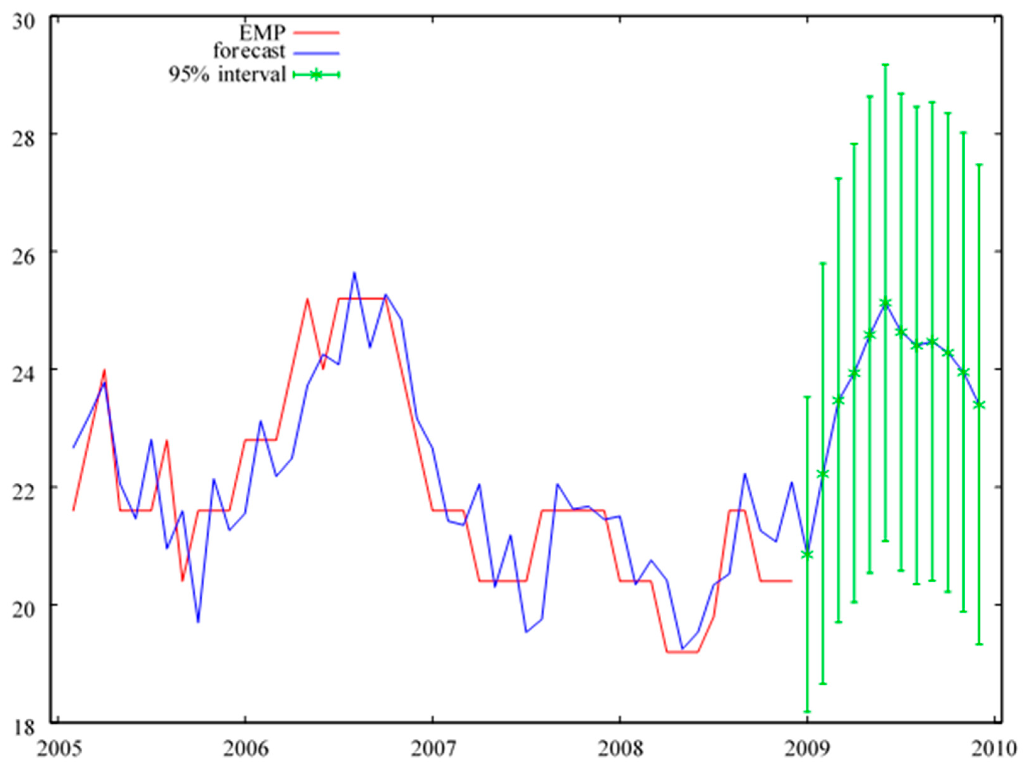
The graphs show forecasts with a 95% confidence interval, which constitutes a computational standard in the widely available, free-of-charge GRETL package. The range boundaries, however, can be changed, depending on the research needs.
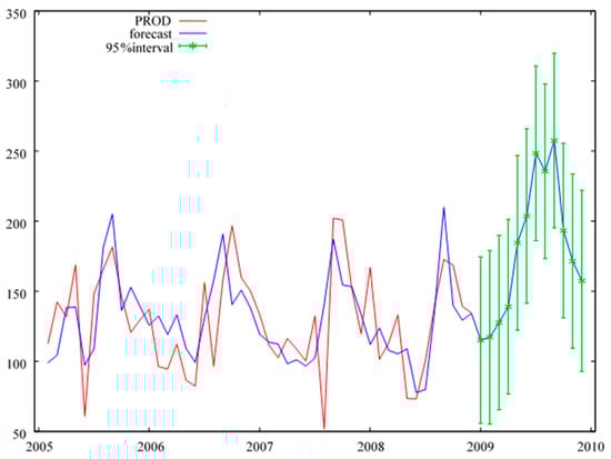
Figure A1.
Monthly forecasts of ready-made production for the year 2009, in a system with an increase in the initial value of machinery and equipment. Source: Table 4.
Figure A1.
Monthly forecasts of ready-made production for the year 2009, in a system with an increase in the initial value of machinery and equipment. Source: Table 4.
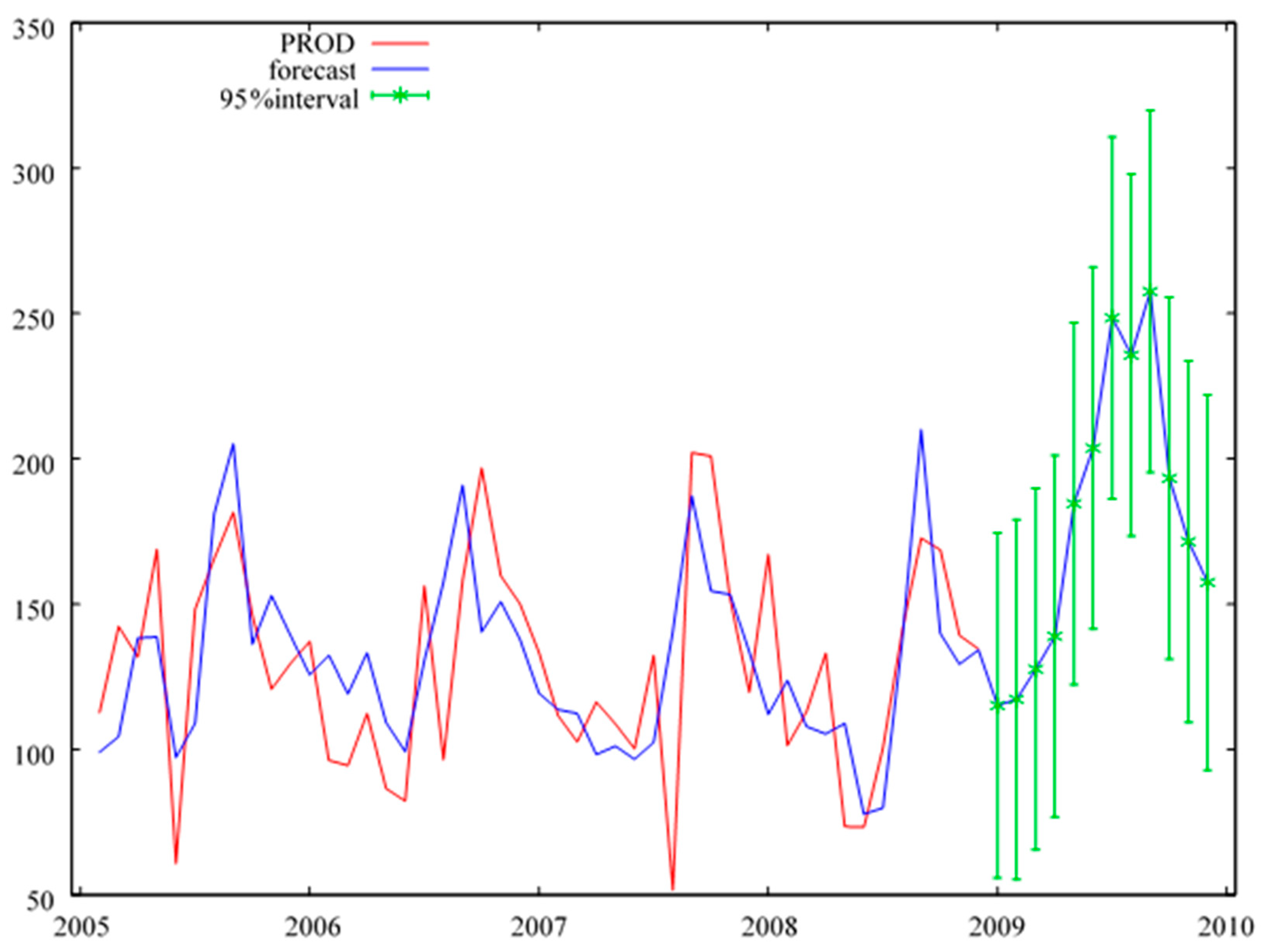
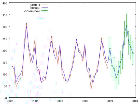
Figure A2.
Monthly forecasts of gross sales revenues for the year 2009, in a system with an increase in the initial value of machinery and equipment. Source: Table 4.
Figure A2.
Monthly forecasts of gross sales revenues for the year 2009, in a system with an increase in the initial value of machinery and equipment. Source: Table 4.
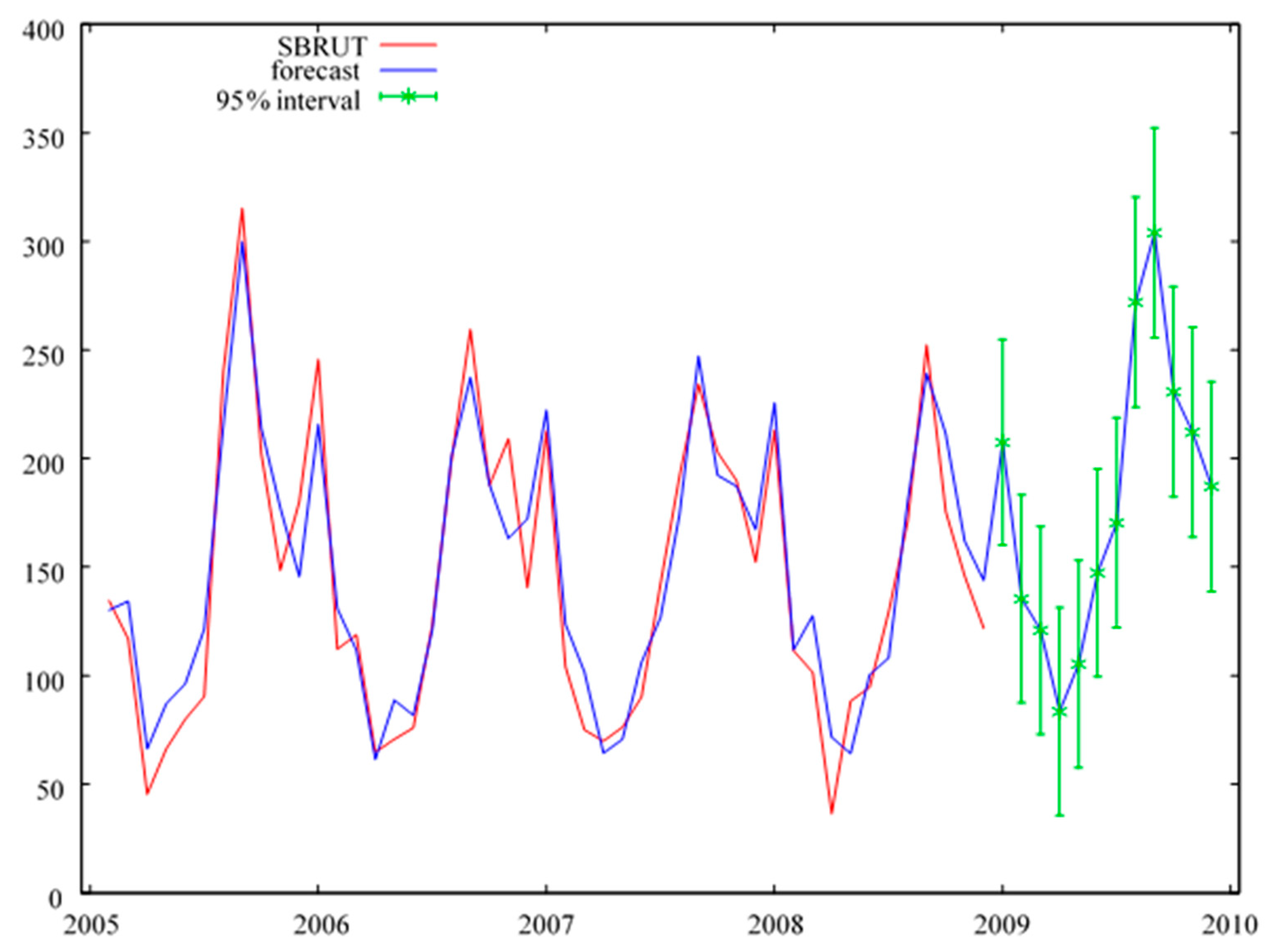
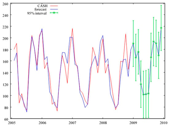
Figure A3.
Monthly forecasts of the cash inflows for the year 2009, in a system with an increase in the initial value of machinery and equipment. Source: Table 4.
Figure A3.
Monthly forecasts of the cash inflows for the year 2009, in a system with an increase in the initial value of machinery and equipment. Source: Table 4.
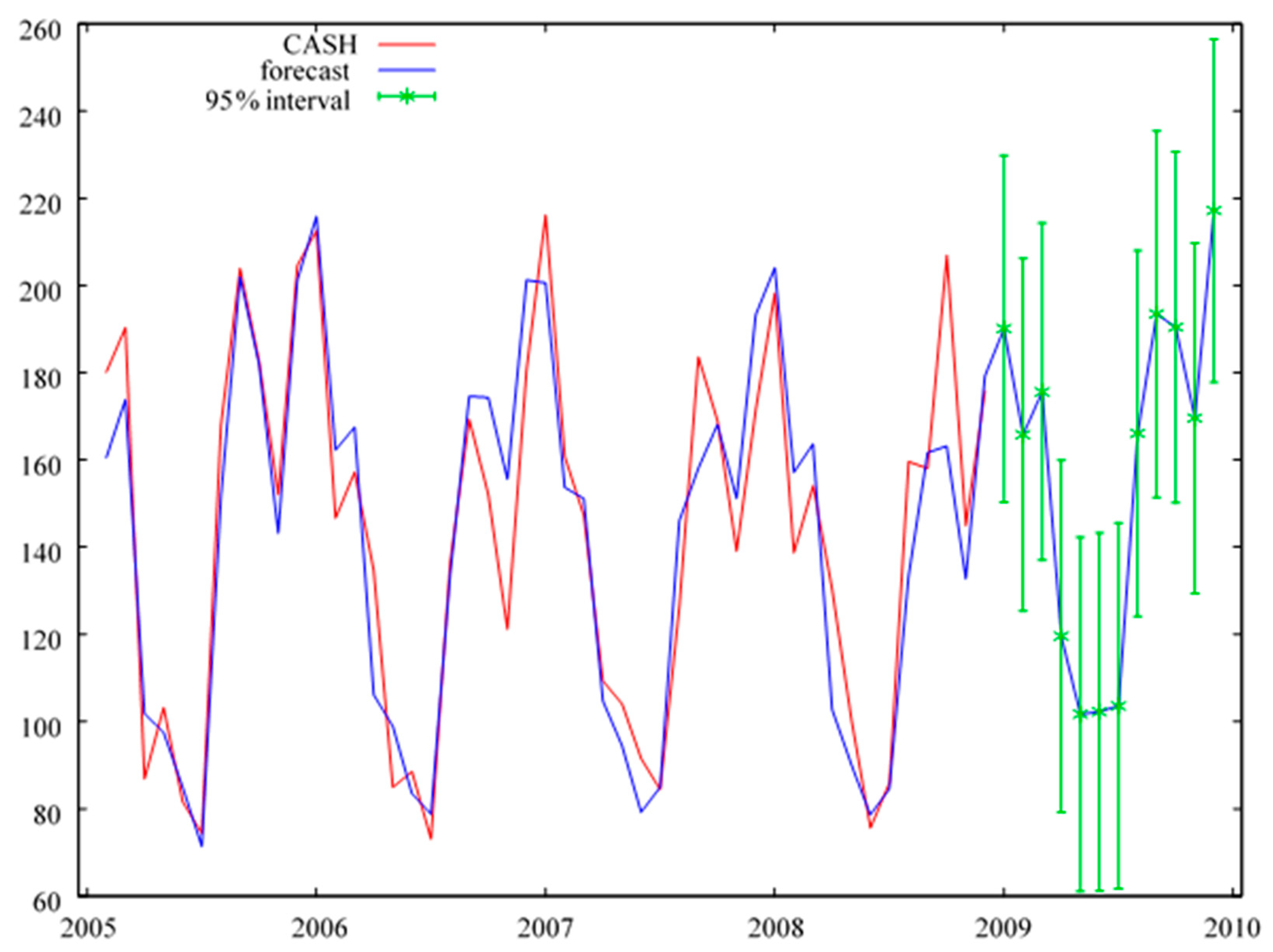
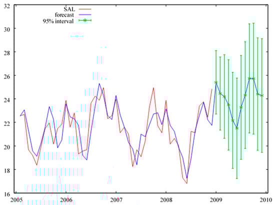
Figure A4.
Monthly forecasts of net pay for the year 2009, in a system with an increase in the initial value of machinery and equipment. Source: Table 4.
Figure A4.
Monthly forecasts of net pay for the year 2009, in a system with an increase in the initial value of machinery and equipment. Source: Table 4.
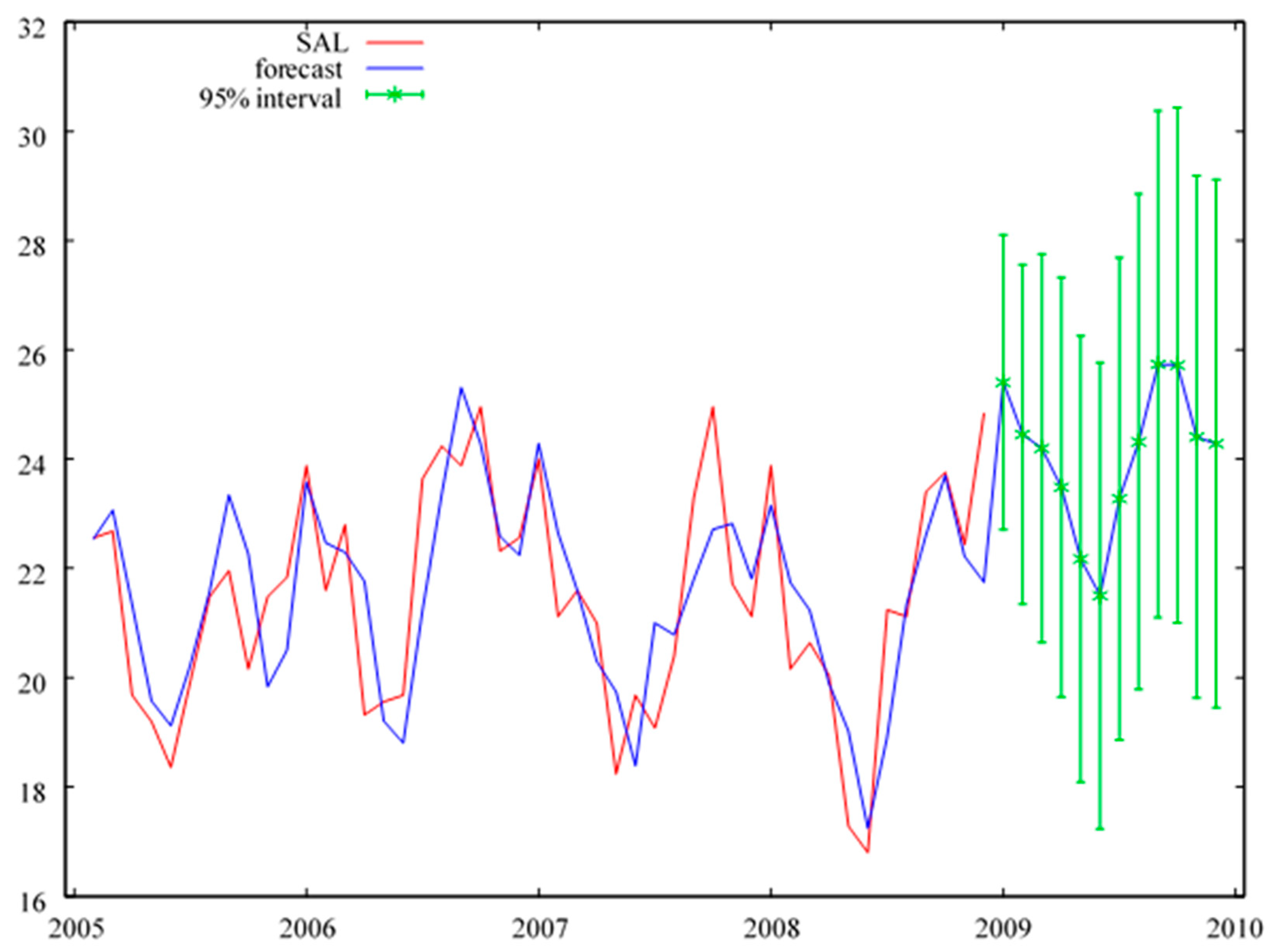
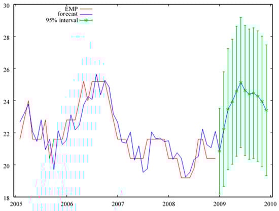
Figure A5.
Monthly forecasts of employment volume for the year 2009, in a system with an increase in the initial value of machinery and equipment. Source: Table 4.
Figure A5.
Monthly forecasts of employment volume for the year 2009, in a system with an increase in the initial value of machinery and equipment. Source: Table 4.
References
- Armstrong, J. Scott. 1984. Forecasting by extrapolation: Conclusions from 25 years of research. Interfaces 14: 52–66. [Google Scholar] [CrossRef]
- Armstrong, J. Scott, and Kesten C. Green. 2017. Forecasting Methods and Principles: Evidence Based Checklists. Available online: https://www.researchgate.net/publication/318392870_Forecasting_Methods_and_Principles_Evidence-Based_Checklists (accessed on 1 December 2017).
- Armstrong, J. Scott, and Rod Brodie. 1999. Forecasting for Marketing. In Quantitative Methods in Marketing, 2nd ed. Edited by Graham J. Hooley and Michael K. Hussey. London: International Thompson Business Press, pp. 92–119. [Google Scholar]
- Beveridge, William H. 1921. Weather and harvest cycles. The Economic Journal 31: 429–52. [Google Scholar]
- Box, George E. P., and Gwilym M. Jenkins. 1970. Time Series Analysis Forecasting and Control. San Francisco: Holden-Day. [Google Scholar]
- Chamberlin, Thomas C. 1965. The method of multiple working hypotheses. Science 148: 754–59. First published 1890. [Google Scholar] [CrossRef] [PubMed]
- Dawid, A. Philip. 1984. Statistical Theory the Prequential Approach. Journal of the Royal Statistical Society: Series A 147: 278–92. [Google Scholar] [CrossRef]
- Graefe, Andreas, Kesten C. Green, and J. Scott Armstrong. 2015. Effect of Conservatism on the Accuracy of Forecasts from Econometric. Paper presented at the International Symposium on Forecasting Riverside, California, CA, USA, June 24. [Google Scholar]
- Harvey, Andrew C. 1989. Forecasting, Structural Time Series Models and the Kalman Filter. Cambridge: Cambridge University Press. [Google Scholar]
- Hawkins, John. 2015. Economic Forecasting: History and Procedures. Available online: https://www.researchgate.net/publication/252956181 (accessed on 15 August 2015).
- Kolmogoroff, Andrei Nikolaevich. 1941. Interpolation und Extrapolation von Stationären zufälligen Folgen. Izvestiya Rossiiskoi Akademii Nauk. Seriya Matematicheskaya 5: 3–14. [Google Scholar]
- Makridakis, Spyros, and Steven C. Wheelwright, eds. 1979. Forecasting. Amsterdam: North-Holland. [Google Scholar]
- Makridakis, Spyros, and Steven C. Wheelwright, eds. 1983. The Handbook of Forecasting. A Manager’s Guide. New York: J. Wiley. [Google Scholar]
- Pankratz, Alan. 1983. Forecasting with Univariate Box–Jenkins Models. Concept and Cases. New York: J. Wiley. [Google Scholar]
- Schnaars, Steven P. 1984. Situational factors affecting forecast accuracy. Journal of Marketing Research 21: 290–97. [Google Scholar] [CrossRef]
- West, Mike, and Jeff Harrison. 1997. Bayesian Forecasting and Dynamic Models. New York: Springer. [Google Scholar]
- Wiener, Norbert. 1949. The Extrapolation, Interpolation and Smoothing of Stationary Time Series with Engineering Applications. New York: J. Wiley. [Google Scholar]
- Wiśniewski, Jerzy W. 2011. Dylematy podwójnej metody najmniejszych kwadratów w mikromodelu ekonometrycznym. In Modelowanie i prognozowanie gospodarki narodowej. Sopot: Prace i Materiały Wydziału Zarządzania Uniwersytetu Gdańskiego, Nr 4/8. pp. 523–30. [Google Scholar]
- Wiśniewski, Jerzy W. 2016a. Microeconometrics in Business Management. New York: John Wiley & Sons. Ltd. Singapore: Chichester. [Google Scholar]
- Wiśniewski, Jerzy W. 2016b. Empirical Econometric Model of an Enterprise. Folia Oeconomica Stetinensia 16: 232–47. [Google Scholar] [CrossRef][Green Version]
- Wiśniewski, Jerzy W. 2017. Predykcja z układu równań współzależnych. Ekonometria Econometrics 1: 9–20. [Google Scholar]
- Wiśniewski, Jerzy W. 2018a. Forecasting from an Econometric Model with Feedback. In 9th International Scientific Conference “Analysis of International Relations 2018. Methods and Models of Regional Development. Winter Edition”. Edited by Włodzimierz Szkutnik, Anna Sączewska-Piotrowska, Monika Hadaś-Dyduch and Jan Acedański. Katowice: Publishing House of the University of Economics in Katowice, pp. 179–85. [Google Scholar]
- Wiśniewski, Jerzy W. 2018b. Forecasting from an Econometric System of Interdependent Equations. Chisinau: LAP LAMBERT Academic Publishing. ISBN 978-3-659-85711-9. [Google Scholar]
- Wiśniewski, Jerzy W. 2020. Prognozowanie z Wielorównaniowych Mikromodeli Ekonometrycznych (Forecasting from Multi-Equation Econometric Micromodels). Toruń: Wydawnictwo Naukowe Uniwersytetu Mikołaja Kopernika. ISBN 978-83-231-4459-5. [Google Scholar]
- Yule, George Udny. 1927. On a method of investigating periodicities in disturbed series with special reference to Wolfer’s sunspot numbers. Philosophical Transactions of the Royal Society of London. Series A 226: 267–98. [Google Scholar]
Publisher’s Note: MDPI stays neutral with regard to jurisdictional claims in published maps and institutional affiliations. |
© 2021 by the author. Licensee MDPI, Basel, Switzerland. This article is an open access article distributed under the terms and conditions of the Creative Commons Attribution (CC BY) license (https://creativecommons.org/licenses/by/4.0/).

