Abstract
Cooling structures of gas turbine blades have become more complex to achieve a better cooling effect. Therefore, heat transfer analysis tools with higher accuracy and efficiency are required to verify the effectiveness of cooling designs and continuously improve the design. In this work, a data-driven method is combined with a decoupled conjugate heat transfer analysis. The analysis object is a typical air-cooled gas turbine first-stage vane with film cooling, impingement cooling, and pin-fin cooling. In addition, a conventional 3-D conjugate heat transfer simulation of the vane was executed for contrast. Results show that this method shortens the time of the heat transfer analysis process significantly and ensures accuracy. It proves that the data-driven method is effective for the evaluation of a modern gas turbine cooling design and is an improvement compared to the traditional three-dimensional heat transfer analysis method.
1. Introduction
For higher thermal efficiency and larger specific work, gas turbines’ inlet temperature rises rapidly and exceeds the allowable temperature of even the best superalloys. The turbine blades of the first several stages must be provided with effective thermal protection to avoid failures. For example, first-stage vanes of a modern gas turbine usually apply the compound scheme with internal impingement cooling, pin-fin cooling, and external film cooling. A complex geometry results in a complex flow, which increases the difficulty of predicting the temperature distribution of gas turbine blades [1,2].
The temperature distribution of the blades is an important criterion for a cooling scheme’s validity during the designing period of a turbine. The peak temperature should not exceed the metal temperature tolerance limit, and the temperature gradient should not be too large to avoid excessive thermal stress on the surface. The solution of the temperature distribution can be abstracted as a heat conduction problem of an infinite one-dimensional plate under the third kind of boundary conditions, convection heat transfer with mainstream hot gas on the outer surface and coolant on the inner surface. The final time-average temperature distribution relies on both conductivity and thermal boundary conditions [3,4]. This is due to the temperature of the blades influencing the flow of the surrounding fluids and may cause the thermal boundary condition to change. This bidirectional influence also makes the prediction of the temperature field more difficult.
A conventional method to obtain the detailed temperature distribution is the conjugate heat transfer calculation. The Navier-Stokes equation is solved in the fluid region, and the Fourier equation is solved in the solid regions. The coupling of two regions is achieved by a common wall temperature and the same heat flux through the intersurface. Bohn et al. [5] developed a conjugate calculation code and used it to calculate the temperature distribution of the convection-cooled nozzle guide vane Mark II. The heat transfer boundary conditions on the air-cooled surface are prescribed with the experimental data; the temperature on the outer surface is fully determined by the conjugate calculation. Finally, the maximum difference in temperature on the outer surface is less than 2%. The conjugate calculation of a film-cooled vane with the same code was also carried out [6]. The results from different film flow angles provided a valuable reference for a film-cooled vanes’ design. Takahashi et al. simulated a real turbine vane with a typical 3-D structure using a commercial conjugate code. The results proved that the conjugate method is useful for the prediction of blade temperature depending on various conditions of operation. Determining the flow and heat transfer in one code is quite convenient. However, the more complicated cooling structure makes the 3-D conjugate heat transfer analysis time-consuming, which is not quite suitable for the optimization design that requires a quick evaluation for a large number of design schemes. It is necessary to develop a relatively accurate cooling-scheme evaluation method that saves time and resources.
In order to make the calculation flexible enough for different accuracy and efficiency demands, a decoupled method was developed, which allows applying different analysis methods to solve different domains. Bonini and Andreini [7,8] developed a cooling system simulation tool combining external CFD, internal flow network code, and a finite element conductive model and applied it to the first rotor blade of the MS5002E gas turbine. Temperature profiles from the simulation tool and experiment matched well. Chowdhury et al. [9] developed a model to calculate the distribution of the coolant mass flow rate and the metal temperatures of a turbine blade, using the mass and energy balance equations at given external and internal boundary conditions. With the application of predicting the temperature distribution of the GE E3 stage 1 blade, this model proved, with reasonable accuracy, if the correct boundary conditions were applied. Ngetich et al. [10] also used the decoupled method to analyze a double-walled turbine blade. The blade was divided into basic units connecting with each other whose internal and external boundary conditions were assigned by correlations. The results from the decoupled method, which include film, metal effectiveness, and coolant mass flow consumption, have been found to closely match results available from the open literature. These decoupled analyses validated the results of each region to timely obtain convinced final results, although the outer iteration between regions is complex [11,12].
In the decoupled analysis method, the models applied in the domains are the key to the final accuracy. The development of the experimental measurement technique [13,14,15] offers a great opportunity for data-driven models based on two-dimensional experimental data, which enables reliable and efficient predictions. This work developed a data-driven method to predict the temperature of gas turbine vanes based on the decoupled heat transfer analysis. The decoupled method is mainly employed for its ability to customize intersurface conditions. The structure of the code allows the flow and heat transfer to interact with each other in a timely manner. The validation of the method was carried out on a typical air-cooled first-stage guide vane. The accuracy and efficiency were assessed by comparing the data-driven method with the fully conjugate calculation andthe experimental data.
2. Data-Driven CHT Method
This section will introduce the data-driven method in detail. Section 2.1. contains the core strategy of the data-driven method concerning the division of regions and the interactiveness between the regions. Section 2.2 introduces the experimental data source and the processing operations. Finally, Section 2.3. describes the integration of the database with the CHT algorithm.
2.1. General Simulation Strategy
The strategy of the data-driven method mainly includes the division method of the regions and the iterative structure of the code.
The outer interface of fluid and solid is the key point in heat transfer analysis. Two sets of domains separated by the outer interface of the vane were chosen for the following analysis. Domain 1 is the passage of hot gas, which is used for the mainstream flow calculation. Domain 2 contains the solid region of the vane and the fluid region inside the vane where coolant flows. The calculation of domain 1 is able to offer mainstream information, which is necessary for heat transfer with film cooling. The other information is obtained from the calculation of Domain 2. The position relationship of the two domains is shown in Figure 1.
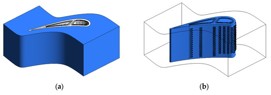
Figure 1.
Domain division: (a) Domain 1; (b) Domain 2.
The interaction between the domains follows the rules in Figure 2. Three parts are for different regions, roughly. In part 1, a simulation of mainstream passage without film cooling on the vane’s surface is carried out. Key parameters of the flow and heat transfer near the vane’s surface were exported for the next parts’ calculations. For the vane and the coolant, a simulation of Domain 2 is carried out to obtain the initial internal flow parameters of the vane. A hypothetical external thermal boundary condition is used in the first simulation of Domain 2 because the actual condition is unknown yet. In part 2, the external thermal boundary condition that consists of the heat transfer coefficient (HTC) and the heat transfer driving temperature (Taw) were generated from the results of the first part. HTC h is a product of HTC without film cooling (h0) and the HTC enhancement factor (h/h0). Equations (1) and (2) were applied for h0′s calculation at the leading edge [16,17],
and the flat board correlation, Equation (3), is for h0 on the pressure surface and suction surface [17].
h/h0 is determined by Baldauf’s method [18]. Taw is calculated by Equation (4) and is assigned to be the heat transfer driving temperature,
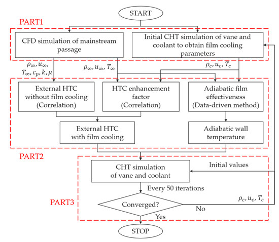
Figure 2.
Iterative strategy of the decoupled CHT method.
Adiabatic film effectiveness η’s distribution on the vane’s surface is generated by the data-driven method using results from part 1, which will be introduced later in Section 2.2.
In part 3, with boundary conditions from part 2, another CFD simulation of Domain 2 is used to obtain new internal flow parameters. These parameters usually differ from those in part 1 due to the different boundary assignments. Therefore, the previous parameters in part 1 were replaced by newly obtained ones, and then part 2 was executed again with new parameters. Such iterations go on until the average temperature variation is less than 0.01 K.
The three parts construct a data-driven method for the heat transfer of the vane’s outer surface. The parameter transfer and iterative calculations ensure the rationality of the final temperature distribution.
2.2. Experimental Database of Film Cooling Effectiveness
The data-driven method in this work considers the film effectiveness distribution on the vane’s surface, a result of the joint influence of multiple units. The basic unit is a single film jet. Each film jet influences its downstream area of a certain width at different degrees, which is determined by the geometry and flow parameters [19]. To describe these influences accurately, a series of data under different sensitive experimental parameters was referenced.
The first step in the data-driven method is to establish a database. Experimental data of a single hole were measured from Qin’s experiment with pressure-sensitive paint (PSP) [20,21]. PSP is an effective surface measurement method that provides a detailed two-dimensional distribution of adiabatic film effectiveness. Its measurement error range is acceptable and known. In this database, data per experimental condition were reshaped to a 61 × 171 matrix corresponding to an area of flow direction coordinates (x/D) ranging from −1 to 16 and lateral coordinates (y/D) ranging from −3 to 3. The total number of data matrices is 440. The experimental conditions were recorded, and their ranges are listed in Table 1. The orthogonal experimental samples provide excellent support for the prediction of film effectiveness based on multiple sensitive parameters.

Table 1.
Experimental conditions in the database.
A sample of adiabatic film effectiveness data matrices is plotted in Figure 3. Since the area affected by the film is a long and narrow strip, the measured data only contains its main area of influence near the hole. The solution to avoid this disadvantage will be introduced in Section 2.3.
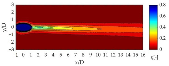
Figure 3.
A sample of experimental data matrix.
2.3. Integration of Database with CHT Algorithm
After simulations in part 1, which were introduced in Section 2.1, the key parameters in Table 1 should be calculated as an input to query the film effectiveness. The multidimensional linear interpolation is implemented according to input parameters. In addition, there is a problem to consider in that the actual coverage of a single hole’s influence is larger than the area’s existing data value. To extract the 2D distribution law and expand it to a larger area, the non-linear least squares regressions were applied with queried data. The detailed method of data extension and the integration with the CHT algorithm is introduced in Section 2.3.
Equation (5) describes the 2-D distribution of cylindrical holes’ film effectiveness in the form of Goldstein’s correlation [22],
When x is assigned, lateral film effectiveness obeys the Gaussian distribution. Strictly, c is also a function of x, but when x is large. The change in c with x is small. Thus, it is considered a constant in the far downstream area. Equation (6) can be deduced from the definition of the lateral averaged film effectiveness () and the integral of ,
Combining Equations (5) and (6) to eliminate , is written as Equation (7),
follows the correlation form in Equation (8). Therefore, the final form of is Equation (9):
If b, c, d, e, and f in Equation (9) are known, the distribution is uniquely defined. The parameters d, e, and f are obtained by regression on data of x/D ranging from 4 to 13, while b and c are decided by regression on data of x/D ranging from 12 to 13. Then, Equation (9) is used to calculate a film effectiveness distribution where x/D is larger than 12.
To make the combination result smooth, the final film effectiveness, where x/D is between 12 and 13, adopts an interpolation from the data queried and the distribution calculated.
The film effectiveness of a fan-shaped hole distributes a little differently from a cylindrical hole. Due to the expansion at the exit, there are usually two peak points in the lateral distribution of film effectiveness. Therefore, the form of is described by the superposition of two Gaussian distributions as Equation (10). Equations (6) and (8) are also suitable for fan-shaped holes. The parameters are determined in the same way as cylindrical holes.
Finally, Sellers’s Equation [23], as below, defined the superposition rules when there are overlaps between film holes’ influence areas:
After the superposition, a complete film effectiveness covering the outer surface of the vane is formed, as shown in Figure 4a,b. The generated film effectiveness distribution is basically consistent with the expected distribution. On the pressure surface, film effectiveness increases along the flow direction because multi-row holes bring coolant accumulation. On the suction surface, film effectiveness keeps declining along the flow direction without continuous coolant supplement.
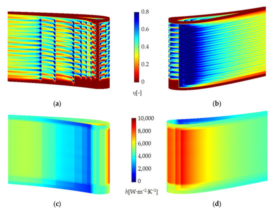
Figure 4.
Boundary conditions generated by the data-driven method: (a) Film effectiveness on pressure surface (-); (b) Film effectiveness on suction surface (-); (c) HTC on pressure surface (W·m−2·K−1); (d) HTC on suction surface (W·m−2·K−1).
The heat transfer enhancement factor (h/h0) is calculated according to single holes’ flow parameters. Superposition rules similar to film effectiveness are applied to form a global distribution in Figure 4c,d.
These surface distributions are written to a (.csv) file to be loaded in preprocessing as a boundary condition. The distribution is recalculated in each new iteration of the data-driven CHT analysis as the key parameters changes.
3. Calculation Analysis
In this section, numerical calculation methods and techniques are introduced, including governing equations, geometric models, mesh selection, calculation settings, etc.
3.1. Governing Equations and Computational Technique
Fluid simulation in this work uses the steady-state RANS method. Three-dimensional steady-state, compressible Reynolds averaged Navier-Stokes equations are solved in the fluid domain. The Solver version is CFX-Solver 19.1. The continuity equation and the momentum equations can be written as
and
respectively. In Equation (13), τ is the stress tensor, and SM is the momentum source term. This work deals with heat transfer, so the total energy equation is also used:
htot is the total enthalpy, and SE is the energy source term. In this work, both momentum and energy source terms can be ignored.
In the solid domain, the following thermal equation is solved instead of the total energy equation:
The velocity of the solid Us is zero in this work.
The SST k-ω turbulence model is used to close the N-S equations after Reynolds averaging. The γ-θ transitional model is set for the fluid domain to obtain a reasonable judgment of transition. The convergence criterion of the traditional coupled heat transfer calculation is that the residual is less than 10−5, and the convergence criterion of the data-driven decoupled calculation method is that the temperature error of the outer iteration is less than 0.01 K.
Two materials are defined for this simulation. The solid’s thermal conductivity (λs) follows a linear expression as Equation (12).
The fluid is an ideal gas. Its thermal conductivity (λf) and dynamic viscosity (μf) are assigned by Sutherland’s formula.
3.2. Vane’s Geometry
One typical guide vane is selected for the validation of the data-driven method. It is modified from the Energy Efficient Engine’s first stage guide vane [24] and has most of the advanced cooling structures. Figure 5 shows its cross-section geometry and cooling structures. The profiles of the sections remain the same along the blade height direction. The vane is fully covered by film cooling holes. Seven rows of cylindrical film holes with 25 degrees of radial inclination are set at the leading edge. Two rows of fan-shaped holes are arranged near the leading edge of the suction surface. Three rows of cylindrical film holes with axial inclination along the axis are on the pressure surface, of which the two rows near the leading edge also have a compound angle. Meanwhile, the vane has a complex internal structure. There are two coolant cavities at different pressures inside the vane with impingement cooling. The cooling structure at the trailing edge includes several rows of pin-fins, which are more usually applied in modern vane designs.
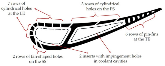
Figure 5.
The geometry and cooling structure of a GE E3 1st Stage Vane.
3.3. Mesh Applied on Calculation
The computing mesh is generated according to the needs of iterative calculations. Three different sets of mesh in Figure 6 are output for certain purposes. The first mesh only contains mainstream passage and the second one includes coolant passage and vane solid. These two are prepared for the data-driven method. The third mesh contains whole computation domains with the mainstream passage, coolant passage, and vane solid. It is prepared for the conventional coupled CHT of the vane together with the mainstream passage.
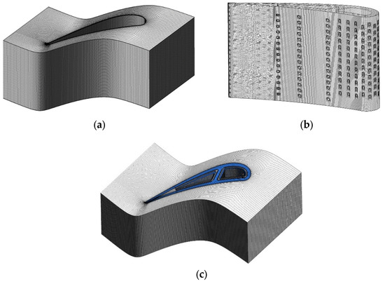
Figure 6.
Mesh for data-driven heat transfer analysis and validation: (a) Mesh 1; (b) Mesh 2; (c) Mesh 3.
For the fluid–solid interfaces and other no-slip walls, the fluid grids nearby are refined to adapt to the turbulence model applied.
The grid independence test is performed against the computational domain, which corresponds to Mesh 3. Three sets of grids with different degrees of density are respectively used for the calculation, and the cell numbers and calculation results are listed in Table 2.
Table 2.
Grid independence test.
The change in mesh density has little influence on the calculation results. Thus, the medium grid density is employed to determine the final grid amount applied. Mesh 1 has 2,099,916 hexahedral cells in total. Most cells of Mesh 2 are also hexahedral except for some solid areas near the film hole where the geometry changes dramatically. The total number of cells in Mesh 2 is 7,422,585. Mesh 3 is not simply a joint of Mesh 1 and Mesh 2. The mesh of the mainstream passage near the exit of the film holes is refined, and the total number of cells exceeds 11,834,831.
3.4. Boundary Set-Ups
The flow parameters are set up according to the design report of the Energy Efficient Engine turbine. For the mainstream inlet, the total pressure is 2.526 MPa, and the total temperature is 2012 K. The Mach number of the mainstream outlet is 0.78. The outlet static pressure recalculated with the isentropic flow hypothesis is 1.51 MPa. The front cavity’s inlet has a higher total pressure of 2.588 MPa. The rear cavity’s inlet has a total pressure of 2.576 MPa. The total temperature at both coolant inlets is 883 K. All boundary conditions about flow are included in Table 3. The hub and shroud are isothermal no-slip walls since the heat transfer of these surfaces is not a concern in this work. Two side surfaces in tangential directions are rotating periodic interfaces. The interface between the fluid and solid is a no-slip wall with heat transfer.
Table 3.
Boundary conditions setup.
4. Results
This section qualitatively analyzes the effect of the data-driven method through the contour map of the calculation results. It then quantitatively evaluates the improvement of the data-driven method compared with the traditional method through the indicators of accuracy and efficiency.
4.1. Temperature Distribution Results
Figure 7 shows the temperature distribution of the vane’s external surface with the conventional CHT method. Referring to the empirical flow pattern of the cascade and film jet, the temperature distribution reasonably reflects the effect of the cooling structure. Film cooling protects most areas of the external surface, except for the top and bottom edges of the suction surface. These areas are controlled by vortices from the endwall, while no film cooling is set on the endwall in this simulation. Therefore, the part close to the middle section of the vane reflects the effect of the blade cooling design. By comparing the temperature distribution on the pressure surface and suction surface, the influence of the film hole type on the cooling effect can be significantly observed. In the case of similar hole spacing, fan-shaped expansion can make the cooling downstream of the hole more uniform. On the pressure surface, the film holes with the compound angle made the coolant accumulate on top of the surface, so the surface temperature decreased along the radial direction. The distribution trend of the traditional CHT is believable due to the features above and the integrity of its analysis domain, but the accuracy of its numerical value is still yet to be discussed.
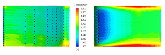
Figure 7.
Temperature distribution of vane’s external surface in conventional method.
Temperature distribution on the external surface of the vane from the data-driven method is shown in Figure 8 with the same legend as Figure 7. Due to the detailed thermal boundary prediction from the data-driven method, the final temperature distribution presents a detailed result similar to that from the conventional CHT. It can obviously be found on the pressure surface that the existence of film holes makes the downstream temperature appear as a band, which means the downstream temperature of the hole is significantly lower than the temperature of the area without air film on both sides. Downstream of the fan-shaped film holes on the suction surface, the uniformity of the temperature distribution of the blade spanwise is consistent with the traditional conjugate calculation, which well captures the cooling characteristics of fan-shaped holes.
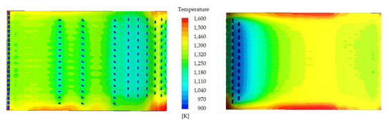
Figure 8.
Temperature distribution of the vane’s external surface in data-driven method.
The overall temperature in Figure 8 is slightly higher than that in Figure 7. Considering that the difference between the two cases lies in the calculation of film cooling, the main reason for the above phenomenon is that the film effectiveness predicted by the data-driven method is relatively lower. When the cooling effect of film on the surface is weakened, the reduction in temperature by internal cooling is more obvious in the cloud image. The low-temperature area on the pressure surface and suction surface near the trailing edge is caused by the enhanced heat transfer of the pin-fins inside the trailing edge. The low-temperature area near the hole outlet is caused by the heat transfer of the hole’s inner wall.
4.2. Performance Evaluation of the Data-Driven Method
This section will analyze in detail the improvement of data-driven methods compared to traditional methods in terms of accuracy and efficiency.
4.2.1. Accuracy
The temperature distribution of the middle section is picked out to form a line diagram in Figure 9. The abscissa is the flow direction arc length calculated from the leading edge, and the ordinate is the temperature of the blade’s metal outer surface. The heat transfer analysis result in the E3 design report is also presented in this figure as a reference. The mean temperature and general trend from the data-driven method are closer to those from the design reports compared to the conventional method.
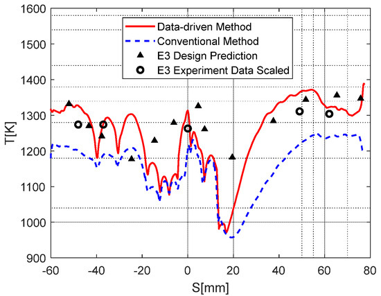
Figure 9.
External surface temperature distribution of the middle section [24,25].
At the arc length position of the experimental data, the temperature calculation errors of the two methods are calculated. Results are shown in Table 4. The maximum error of the data-driven method is about 53.3 K, corresponding to a relative error of 4.1%. The maximum error of the conventional method is about −92.7 K, corresponding to a relative error of −7.1%. The minus sign means that the calculation result is lower than the test result. For the conventional method, the low prediction temperature may be mainly due to the high prediction of the downstream film effectiveness by CFD. By citing the experimental data of film effectiveness, the data-driven method avoids the inherent problem of low wall temperature caused by CFD and effectively improves the accuracy of temperature prediction.
Table 4.
Calculation error of the middle section temperature.
4.2.2. Computational Cost
The computations are both made with 36 processes on the same server. The data-driven method takes 5 h and 21 min, while the conventional CHT method takes 17 h and 49 min, which is three times larger than the data-driven one. This is more obvious in Table 5 with the same units. The application of the data-driven method can save 69.97% of heat transfer analysis time. High efficiency is a significant advantage of the data-driven method. The computational cost will be less if this method is spread to predict the internal boundary conditions.
Table 5.
Time cost.
5. Conclusions
At present, the heat transfer prediction of gas turbine blades with a complex cooling structure is difficult and time-consuming. Under this background, a data-driven conjugate analysis method is proposed in this paper. Different from the traditional coupling CHT method, this method uses a decoupled method, which computes different domains with different methods. The data transfer between the domains is realized through the iteration of the outer cycle. In the process of the outer iteration, the data-driven prediction model of film cooling is applied at the conjugate boundary. The data-driven prediction model of film cooling is based on the film cooling unit experimental database under the influence of multiple parameters, and the data is modified and extended to predict the film cooling effect applied to the cascade surface.
In this paper, a typical first-stage vane based on the E3 turbine is selected for validation. The temperature distribution calculated by the data-driven method is similar to that of the conventional method, which can correctly reflect the influence of the typical cooling structure on the solid wall temperature. Compared with the conventional method, the temperature distribution of the blade mid-section calculated by the data-driven method is in better agreement with the experimental data. This means that the data-driven method effectively avoids the overestimation of the film cooling effectiveness of the conventional CHT, and its prediction accuracy can support the effectiveness evaluation of the cooling scheme. In addition, compared with the traditional coupled CHT, the analysis efficiency of the data-driven method is also significantly improved. This reduction in heat transfer analysis time enables more iterations of cooling designs in the same amount of time, and further efficiency improvements in this direction will hopefully support the optimization design based on higher prediction accuracy.
Author Contributions
Conceptualization, supervision, X.L. and J.R.; investigation, methodology, validation, H.C. and L.W.; data curation, visualization, H.C.; writing—original draft preparation, H.C.; writing—review and editing, X.L. and J.R. All authors have read and agreed to the published version of the manuscript.
Funding
This research was funded by National Science and Technology Major Project, grant number J2019-III-0007-0050.
Data Availability Statement
Not applicable.
Conflicts of Interest
The authors declare no conflict of interest.
References
- Bunker, R.S. Evolution of Turbine Cooling. In Proceedings of the ASME Turbo Expo 2017: Turbomachinery Technical Conference and Exposition, Volume 1: Aircraft Engine; Fans and Blowers; Marine; Honors and Awards, Charlotte, NC, USA, 26–30 June 2017. [Google Scholar] [CrossRef]
- Han, J. Turbine Blade Cooling Studies at Texas A&M University: 1980–2004. J. Thermophys. Heat Transf. 2006, 20, 161–187. [Google Scholar] [CrossRef]
- Heidmann, J.D.; Kassab, A.J.; Divo, E.A.; Rodriguez, F.; Steinthorsson, E. Conjugate Heat Transfer Effects on a Realistic Film-Cooled Turbine Vane. In Proceedings of the ASME Turbo Expo 2003, Collocated with the 2003 International Joint Power Generation Conference, Volume 5: Turbo Expo 2003, Parts A and B, Atlanta, GA, USA, 16–19 June 2003. [Google Scholar] [CrossRef]
- Zecchi, S.; Arcangeli, L.; Facchini, B.; Coutandin, D. Features of a Cooling System Simulation Tool Used in Industrial Preliminary Design Stage. In Proceedings of the ASME Turbo Expo 2004: Power for Land, Sea, and Air, Volume 3: Turbo Expo 2004, Vienna, Austria, 14–17 June 2004. [Google Scholar] [CrossRef]
- Bohn, D.; Bonhoff, B.; Schrinenbom, H. Combined Aerodynamic and Thermal Analysis of a Turbine Nozzle Guide Vane. In Proceedings of the 1995 Yokohama International Gas Turbine Congress, Yokohama, Japan, 22–27 October 1995. [Google Scholar]
- Bohn, D.E.; Becker, V.J.; Kusterer, K.A. 3-D Conjugate Flow and Heat Transfer Calculations of a Film-Cooled Turbine Guide Vane at Different Operation Conditions. In Proceedings of the ASME 1997 International Gas Turbine and Aeroengine Congress and Exhibition, Volume 3: Heat Transfer; Electric Power; Industrial and Cogeneration, Orlando, FL, USA, 2–5 June 1997. [Google Scholar] [CrossRef]
- Bonini, A.; Andreini, A.; Carcasci, C.; Facchini, B.; Ciani, A.; Innocenti, L. Conjugate Heat Transfer Calculations on GT Rotor Blade for Industrial Applications: Part I—Equivalent Internal Fluid Network Setup and Procedure Description. In Proceedings of the ASME Turbo Expo 2012: Turbine Technical Conference and Exposition, Volume 4: Heat Transfer, Parts A and B, Copenhagen, Denmark, 11–15 June 2012. [Google Scholar] [CrossRef]
- Andreini, A.; Bonini, A.; Da Soghe, R.; Facchini, B.; Ciani, A.; Innocenti, L. Conjugate Heat Transfer Calculations on GT Rotor Blade for Industrial Applications: Part II—Improvement of External Flow Modeling. In Proceedings of the ASME Turbo Expo 2012: Turbine Technical Conference and Exposition, Volume 4: Heat Transfer, Parts A and B, Copenhagen, Denmark, 11–15 June 2012. [Google Scholar] [CrossRef]
- Chowdhury, N.H.K.; Zirakzadeh, H.; Han, J. A Predictive Model for Preliminary Gas Turbine Blade Cooling Analysis. J. Turbomach. 2017, 139, 091010. [Google Scholar] [CrossRef]
- Ngetich, G.C.; Murray, A.V.; Ireland, P.T.; Romero, E. A Three-Dimensional Conjugate Approach for Analyzing a Double-Walled Effusion-Cooled Turbine Blade. J. Turbomach. 2019, 141, 011002. [Google Scholar] [CrossRef]
- Amaral, S.; Verstraete, T.; Braembussche, R.V.; Arts, T. Design and Optimization of the Internal Cooling Channels of a High Pressure Turbine Blade—Part I: Methodology. J. Turbomach. 2010, 132, 021013. [Google Scholar] [CrossRef]
- Verstraete, T.; Amaral, S.; Braembussche, R.V.; Arts, T. Design and Optimization of the Internal Cooling Channels of a High Pressure Turbine Blade—Part II: Optimization. J. Turbomach. 2010, 132, 021014. [Google Scholar] [CrossRef]
- Zhang, L.J.; Jaiswal, R.S. Turbine nozzle endwall film cooling study using pressure-sensitive paint. J. Turbomach. 2001, 123, 730–738. [Google Scholar] [CrossRef]
- Gao, Z.; Wright, L.M.; Han, J. Assessment of Steady State PSP and Transient Ir Measurement Techniques for Leading Edge Film Cooling. In Proceedings of the ASME 2005 International Mechanical Engineering Congress and Exposition, Heat Transfer, Part A, Orlando, FL, USA, 5–11 November 2005; pp. 467–475. [Google Scholar] [CrossRef]
- Gao, Z.; Han, J. Influence of Film-Hole Shape and Angle on Showerhead Film Cooling Using PSP Technique. J. Heat Transf. 2009, 131, 061701. [Google Scholar] [CrossRef]
- Lowery, G.W.; Vachon, R.I. The Effect of Turbulence on Heat Transfer from Heated Cylinders. Int. J. Heat Mass Transf. 1975, 18, 1229–1242. [Google Scholar] [CrossRef]
- Kreith, F.; Manglik, R.M. Principles of Heat Transfer, 8th ed.; Cengage Learning: Boston, MA, USA, 2018; pp. 342+362. [Google Scholar]
- Baldauf, S.; Scheurlen, M.; Schulz, A.; Wittig, S. Heat flux reduction from film cooling and correlation of heat transfer coefficients from thermographic measurements at enginelike conditions. J. Turbomach. 2002, 124, 699–709. [Google Scholar] [CrossRef]
- Bogard, D.G.; Thole, K.A. Gas Turbine Film Cooling. J. Propul. Power 2006, 22, 249–270. [Google Scholar] [CrossRef]
- Qin, Y.; Ren, J.; Jiang, H. Effects of Streamwise Pressure Gradient and Convex Curvature on Film Cooling Effectiveness. In Proceedings of the ASME Turbo Expo 2014: Turbine Technical Conference and Exposition, Volume 5B: Heat Transfer, Düsseldorf, Germany, 16–20 June 2014. [Google Scholar] [CrossRef]
- Qin, Y.; Li, X.; Ren, J.; Jiang, H. Effects of compound angle on film cooling effectiveness with different streamwise pressure gradient and convex curvature. Int. J. Heat Mass Transf. 2015, 86, 482–491. [Google Scholar] [CrossRef]
- Goldstein, R.J. Film Cooling. Adv. Heat Transf. 1971, 7, 321–379. [Google Scholar] [CrossRef]
- John, P.; Sellers, J.R. Gaseous Film Cooling with Multiple Injection Stations. AIAA J. 1963, 1, 321–379. [Google Scholar] [CrossRef]
- Halila, E.E.; Lenahan, D.T.; Thomas, T.T. Energy Efficient Engine High Pressure Turbine Test Hardware Detailed Design Report; Report No.: NASA CR-167955; NASA: Washington, DC, USA, 1982; pp. 23–34.
- Stearns, E.M. Energy Efficient Engine Core Design and Performance Report; Report No.: NASA CR-168069; NASA: Washington, DC, USA, 1982; pp. 357–361.


Publisher’s Note: MDPI stays neutral with regard to jurisdictional claims in published maps and institutional affiliations. |
© 2022 by the authors. Licensee MDPI, Basel, Switzerland. This article is an open access article distributed under the terms and conditions of the Creative Commons Attribution (CC BY) license (https://creativecommons.org/licenses/by/4.0/).