Thermodynamic Optimization of Aircraft Environmental Control System Using Modified Genetic Algorithm

Abstract

This paper presents an optimization method for the civil aircraft environmental control system (ECS) mainly involving two airstreams: the ram airstream for cooling and the bleed airstream for supplying the cabin. The minimum total fuel energy consumption rate (FECR), defined as the weighted sum of the shaft power extraction and propulsive power loss, is obtained under the precondition of the constant outputs in the cooling capacity and outlet pressure. A modified genetic algorithm (GA) is proposed to acquire the optimal values of the heat transfer areas, temperature ratio of bleed air, mass flow rate of ram air, and pressure ratios of the turbine, compressor, and fan. The statistical results show that the multipoint crossover and continuity improvement implemented in the modified GA improve convergence and distribution performance. The probability of reaching a satisfactory result using modified GA is 62.4% higher than standard GA. Due to the decrease of inlet parameters of bleed air and the elimination of power input in the compressor, the FECR of the optimization case can be lowered by 11.0%. In general, the evaluation method considering energy quality together with the modified optimization technique is proved effective in energy-saving design for such energy systems such as ECS with multiple inputs and outputs.

1. Introduction

Energy conservation and thermal management for aircraft have been hot issues for the last decades. Since aviation contributes a considerable share of 2.2% to the global energy consumption [1], relevant researches focus on the propulsion system and some accessory systems aiming for lower CO₂ emission [2,3]. The environmental control system (ECS) is a typical accessory system of aircraft that consumes the energy from the aero-engine. Its efficiency highly affects the energy consumption of the aircraft. ECS is mainly in charge of maintaining the aircraft environment (temperature, pressure, and air composition) within acceptable limits [4]. The air supply, thermal control, and cabin pressurization are realized in the system by relevant components, mainly including the compressor, turbine, heat exchanger, intake, and exhaust subsystems. Since the appearance of the earliest aircraft ECS to face the low pressure caused by the rising flight height in the 1940s, environmental control technologies have been developing continuously [5]. In the last decades, the ECSs evolved from double-wheel types, including simple type [6,7,8,9] and bootstrap type [10,11,12,13,14,15,16,17,18,19,20], to three-wheel [21,22,23,24] and four-wheel type [25], then from conventional types with bleed air to electric type [21,25,26].

With the increasing attention to the efficiency of energy systems, parametric optimization has become a necessary design tool to reduce energy consumption. It inspired many scholars to do lots of research in this field. Different optimization criteria and methods were selected and developed for ECS under both steady and transient conditions. Cui [21] optimized three types of ECS by taking exergy destruction and univariate optimization as the optimization criterion and method. The effects of compressor and turbine parameters on the exergy loss were obtained individually. Li et al. [9] investigated the ECS heat exchanger optimization based on the entropy generation analysis. Several vital structural parameters were separately optimized, and the design method for the ECS heat exchanger was proposed. Vargas et al. [10] developed a mathematical model for an aircraft ECS, through which the minimum entropy generation was obtained by changing its structural parameters. Alebrahim et al. [11] compared the thermodynamic irreversibility between two configurations of ECS with the difference in the heat exchanger arrangement. The optimal design with minimum entropy generation rate was provided for each configuration. Ordonez et al. [12] optimized four models of ECS. Two fundamental issues in the thermodynamic optimizations of ECS were considered, including the limits for the minimum power requirement and the design features that facilitate operation at minimal power consumption. The relation of the total power requirement to exergy loss was obtained. In the optimization of Pérez-Grande et al. [13], two objective functions were analyzed, including the heat exchanger volume and the entropy generation number. It was difficult to determine the optimal configuration as the optimization results obtained from two objective functions had opposite trends. Similarly, Vargas et al. [14] also selected exergy destruction and total power requirement as the optimization criteria. The optimal systematic configuration changed along with the given objective. Such relation between optimal designs and multiple objective functions can also be found in other research about energy systems [27,28,29] with a “trade-off” method to balance different objective functions.

Most of the work listed above adopts the univariate optimization method, in which only a single variable changed continuously while other variables kept constant. Therefore, the coupling effect of multiple variables on the objective function cannot be studied deeply. In view of this, Li et al. [20] used the heat current method to analyze the ECS performance. The takeoff gross weight was optimized with Lagrange multiplier method considering multiple variables, including heat exchanger areas and mass flow rates. Yang et al. [26] developed the multivariate power optimization on electric ECS. Mathematical optimization formulation was proposed for energy conservation. Shiba et al. [30] conducted the multivariate optimization of ECS by changing the length and mass flow rate of a counter-flow heat exchanger simultaneously. The dimensionless ratio of the total power requirement to the refrigeration load was chosen as the objective function to acquire the optimal heat exchanger structure. Sanaye et al. [31] also used multivariate optimization tool to optimize a plate-fin heat exchanger with genetic algorithm. The maximum effectiveness and minimum total cost were obtained by considering six structural variables. In addition to the above research of steady-state optimization, there were also some transient studies on ECS. Zhao et al. [19] performed a transient experiment of ECS to reveal the systematic characteristics and its dynamic response under different flight altitudes. Tu et al. [22] established a transient model for a three-wheel ECS using Flowmaster software. The dynamical response of cabin-zone temperature is simulated and a fuzzy-theory-based controller is designed for it.

From above literature review, the exergy destruction [21,23,32], entropy generation [9,10,11,12,13,16,17,18], and total power requirement [12,13,14,29] were the most common optimization criteria for the steady-state optimization of ECS. Among them, the physical meanings of exergy destruction and the entropy generation were similar. The definitions of total power requirement varied in different investigations. However, with regard to the specific energy system ECS, these criteria are not completely appropriate or should be applied with additional limitations. ECS has multiple inputs and outputs. It gives the aircraft cabin an airstream with suitable temperature and pressure, consuming propulsive power and shaft power from aero-engine. So, ECS outputs are difficult to quantify in the form of energy, distinguished from the outputs of aero-engine and gas turbine generator, which are suitable to be quantified by propulsive power and generation power, respectively. As for the inputs, different pressure potential energy and thermal energy are extracted into different airstreams. Therefore, these commonly used criteria are insufficient to evaluate ECS with multiple inputs and outputs in different energy qualities. In view of this, an appropriate evaluation method is needed for such energy systems.

The output of ECS is defined by two parameters, cooling capacity (related to outlet temperature) and outlet pressure. It means there should be at least two variables changing simultaneously to keep the output constant. Therefore, multivariate optimization is required to maintain constant output and reveal the coupling effects of multiple variables. In terms of the number of variables from the above literature review, univariate optimization [9,10,11,12,13,14,16,21,23,32] was widely used to discuss the influence of a single variable on the system performance. Multivariate optimization tool was adopted in only a few research about ECS, and most of them were conducted for its crucial component such as heat exchanger [18,30,31,33]. While in energy-related fields, it is common to employ multivariate optimization [34,35,36,37] solved by particle swarm optimization [34], genetic algorithm [35,36,37,38,39,40,41], etc. The genetic algorithm (GA) is an effective optimization method for energy research, and the performance of GA itself has been improved by many scholars. Mo [36] developed a hybrid GA by implementing Niche technique to avoid the concentration of offspring. Ozcelik [38] programmed a real-coded GA with an improvement of mixing the discrete and continuous variables. Elitist preservation [39,40] and artificial neural network (ANN) [41] are also applied to improve GA.

Based on the above issues, the present work proposes a novel evaluation method of energy efficiency for such energy systems such as ECS with multiple inputs and outputs in different energy quality. In this method, the inputs of ECS are defined as total fuel energy consumption, which is the weighted sum of the propulsive power loss and shaft power extraction according to their energy quality traced back to fuel combustion. The output of ECS is set constant to meet the requirement and avoid its unquantifiable characteristic. With the target of minimum energy consumption under the same output, the multivariate optimization of a civil aircraft ECS is conducted to simultaneously obtain the optimal values of seven key design variables, including the heat exchanger areas, mass flow rate of ram air, inlet parameters of bleed air, and pressure ratios of three turbomachines. To rapidly and accurately obtain the optimal systematic configuration, this work also develops a modified binary-coded GA with better convergence through implementing the multipoint crossover and continuity improvement.

2. Materials and Methods

A conventional three-wheel environmental control system, which has been applied in the aircraft A330/A340 and B757 [5], is selected as the analysis object in the present work. Here, “conventional” refers to that the air for supplying the cabin comes from the core engine, not from the atmosphere compressed by the electric devices. A three-wheel ECS refers to an ECS with a turbine that drives a compressor and a fan simultaneously. The schematic of the ECS is given in Figure 1, where P-HX, S-HX, Com., and Heat Re. represent the primary heat exchanger, secondary heat exchanger, compressor, and heat regenerator, respectively.

There are two airstreams involved in the ECS, identified as the ram airstream and bleed airstream. For the former (thick hollow arrow from node 1 to node 10), the ram air enters the ECS through the diffuser. Then it successively flows through the secondary and primary heat exchangers to cool the bleed air from the core engine. After heat transfer process, the flow is pressured by the fan and then expanded in the nozzle to provide some thrust for the aircraft. It can be found that the primary function of the ram airstream is to provide the cooling air with a certain impact on the thrust.

Another stream is the bleed airstream shown as the thin arrow representation from node 11 to node 30. The bleed air taken from the intermediate stage of the high-pressure compressor is firstly cooled against the ram air in the primary heat exchanger. Then it is pressured in the compressor and cooled through the secondary heat exchanger, heat regenerator and condenser. After that, the air with high pressure and low temperature becomes dehumidified and reheated successively. Finally, the bleed air is expanded and further cooled in the turbine, then enters the cabin with suitable pressure and temperature. As the key flow path of ECS, the bleed airstream provides the fresh air to maintain the basic need of passengers.

The energy inputs of ECS are contained in the above two inputted airstreams. The ram airstream is pressurized at the cost of propulsive power from aeroengine, while the bleed airstream is directly powered by the engine. The output is the bleed airstream after expanded and cooled at node 30. Thus, the optimization conducted on ECS is to save the energy consumption from the engine when the output keeps constant.

2.1. Component-Level Model and Verification

The governing equations are given according to different components to solve the systematic parameters. The key components involved in the proposed ECS include diffuser, nozzle, heat exchanger, compressor, turbine, and their connecting pipelines. Their models and the corresponding verification are presented in this subsection.

Diffuser and nozzle are applied in the intake and exhaust subsystems. According to the different inputs for two components, the outlet parameters can be determined by the outlet Mach number or pressure ratio:

Diffuser:

$$T_{out}=T_{in}\left(1+\frac{\kappa -1}{2}M{a}^2\right)$$

(1)

$$p_{out}=p_{in}{\left[1+{\eta }_d\left(\frac{\kappa -1}{2}M{a}^2\right)\right]}^{\frac{\kappa }{\kappa -1}}$$

(2)

Nozzle:

$$T_{out}=T_{in}\left\{1-{\eta }_n\left[1-{\left(p_{out}/p_{in}\right)}^{\frac{\kappa -1}{\kappa }}\right]\right\} \left(p_{out}/p_{in}\le 1.893\right)$$

(3)

$$T_{out}=T_{in}\left\{1-{\eta }_n\left[1-{1.893}^{\frac{\kappa -1}{\kappa }}\right]\right\} (p_{out}/p_{in}>1.893)$$

(4)

where η_d and η_n represent the efficiency of diffuser and nozzle, κ represents the heat capacity ratio of air. Relevant symbols are listed in Nomenclature.

As the central thermal control unit of ECS, the heat exchangers, including the primary heat exchanger, secondary heat exchanger, regenerator, and condenser, are calculated based on the NTU method:

$$\mu =m_{hot}{c}_p/m_{cold}{c}_p$$

(5)

$${\eta }_{HX}=1-\exp \left\{\mu NT{U}^{0.22}\left[\exp \left(-\frac{1}{\mu }NT{U}^{0.78}\right)-1\right]\right\}$$

(6)

$${\eta }_{HX}=\mu \left(T_{cold,out}-T_{cold,in}\right)/\left(T_{hot,in}-T_{cold,in}\right)$$

(7)

where NTU is the number of heat transfer units, η_HX is the effectiveness of heat exchanger, μ is the ratio of heat capacity rates. In the present case, m_coldc_p is always higher than m_hotc_p.

For turbomachinery, the outlet temperature is mainly related to the pressure ratio:

Compressor and fan:

$$T_{out}=T_{in}\left\{1+\left(1/{\eta }_c\right)\left[{\left(p_{out}/p_{in}\right)}^{\frac{\kappa -1}{\kappa }}-1\right]\right\}$$

(8)

Turbine:

$$T_{out}=T_{in}\left\{1-{\eta }_t\left[1-{\left(p_{out}/p_{in}\right)}^{\frac{\kappa -1}{\kappa }}\right]\right\}$$

(9)

where η_c is the adiabatic efficiency of the compressor or fan, η_t is the adiabatic efficiency of the turbine.

To match the pressure ratios of turbomachines, the turbine shaft power W_t can be expressed as the sum of the compressor power and fan power:

$$W_t=W_c+W_f$$

(10)

The pressure drop in the connecting pipeline is considered in the ECS model:

$$\Delta p=\lambda ·\left(L/D\right)·\left(\rho v^2/2\right)$$

(11)

$$\lambda =64/Re\left(Re\le 2000\right)$$

(12)

$$\lambda =0.3164/R{e}^{0.25}(Re>2000)$$

(13)

$$Re=vd\rho /{\mu }_a$$

(14)

where λ is the resistance coefficient, L is the length of the pipeline, D is the diameter of the pipeline, v is the average velocity.

According to the mentioned component-level models and boundary conditions, each component’s inlet and outlet parameters can be determined in sequence. A comparison of the adopted simulation method with the published work [21] is carried out to verify the model. The results shown in

Table 1. Comparison between the results of the present paper and the corresponding results of Ref. [21].

Node	Ref. [21]		Present Paper		Difference (%)
	T [K]	p [kPa]	T [K]	p [kPa]	ΔT	Δp
11	485	210	485	210	0.00	0.00
13	375.8	205	372.8	205	−0.80	0.00
15	437.4	307.5	433.8	307.1	−0.82	−0.13
17	295.1	303.5	292.6	303.9	−0.85	0.13
19	265.9	299.7	260.9	299.3	−1.88	−0.13
21	242	296.2	239.6	296.1	−0.99	−0.03
25	271.1	290.2	271.3	289.4	0.07	−0.28
27	209.9	90.7	210.0	90.4	0.05	−0.33
29	233.5	88.2	231.2	88.4	−0.99	0.23

present that the deviations between the two models are acceptable.

2.2. Thermo-Economics Criterion

This work aims to optimize the proposed ECS in civil aircraft. The optimization is conducted from the thermo-economics point of view to reduce the required energy input that operates the ECS with constant outputs.

The power source for operating ECS is the high-pressure bleed air from the intermediate compressor, which is driven by the turbine. The ram air is pressurized at the cost of propulsive power. Thus all types of energy in ECS, including mechanical energy and internal energy, can be considered originated from fuel combustion. It is reasonable to consider the total energy consumption as the sum of different forms of energy [42]. With regard to ECS, the total energy consumption mainly includes the following contents: energy consumption of the bleed air, the ram air, and the increased weight of the heat exchangers.

(1) The energy consumption of the bleed air

Since the bleed air is taken from the intermediate stage of the high-pressure compressor, its total energy consumption can be obtained by the sum of the consumed energy for the bleed air against the resistance in the diffuser and for raising the pressure of the bleed air.

The power consumption in the diffuser at a fixed flight Mach number Ma is calculated by:

$$E_{d,bleed}=m_{bleed}·{\left(\sqrt{\kappa R{T}_{0,s}}·Ma\right)}^2/{\eta }_p$$

(15)

where m_bleed is the mass flow rate of the bleed air that meets the ECS needs, T_0,s is the ambient static temperature, η_p is the propulsive efficiency set to 0.356 [43].

The fuel energy consumption of the compression process for the bleed air can be determined by:

$$E_{c,bleed}=m_{bleed}{h}_{bleed}/{\eta }_{th}$$

(16)

where h_bleed is the specific enthalpy of the inlet bleed air and η_th is the thermal efficiency of the core engine that is set to 0.55 [43].

Taking ambient total temperature T₀ as reference temperature, the specific enthalpy of the inlet bleed air is given by:

$$h_{bleed}=c_p·\left(T_{bleed}-T_0\right)$$

(17)

$$T_0=T_{0,s}·\left(1+\frac{\kappa -1}{2}M{a}^2\right)$$

(18)

where T_bleed is the inlet total temperature of the bleed air.

Sum up the above equations, the total energy consumption of the bleed air can be obtained from:

$$\begin{gathered} E_{bleed air}=E_{d,bleed}+E_{c,bleed} \\ =m_{bleed}{\left(Ma\sqrt{\kappa R{T}_{0,s}}\right)}^2/{\eta }_p+c_p{m}_{bleed}\left(T_{bleed}-T_{0,s}\left(1+\frac{\kappa -1}{2}M{a}^2\right)\right)/{\eta }_{th} \end{gathered}$$

(19)

(2) The energy consumption of the ram air

The ram air directly enters ECS with ambient total temperature and total pressure at the cost of producing a specific resistance. Its driving force is from the fan powered by the bleed air and the propulsive power generated by the core engine. The fan power is already counted in the energy consumption of bleed air, and the partial propulsive power is used to overcome the resistance in the diffuser of ECS. Furthermore, the nozzle of ECS can provide specific propulsive power by accelerating the ram air. Therefore, the energy consumption of the ram air is the difference between the power consumption in the diffuser and the propulsive power gained in the nozzle.

Similar to the diffuser of the core engine, the energy consumption to overcome the resistance of the ram air flow in the ECS diffuser can be given by:

$$E_{d,ram}=m_{ram}·{\left(\sqrt{\kappa R{T}_{0,s}}·Ma\right)}^2/{\eta }_p$$

(20)

where m_ram is the mass flow rate of the ram air.

After the heat transfer processes in the heat exchanger and pressurization in the fan, the ram air is expanded in the nozzle. The energy saving in the expansion process is determined by:

$$E_{n,ram}=m_{ram}{v}_{out}·\sqrt{\kappa R{T}_{0,s}}·Ma/{\eta }_p$$

(21)

where v_out is the exhaust velocity of the ECS nozzle.

According to the above equations, the total energy consumption of the ram air can be summarized as:

$$E_{ram air}=E_{d,ram}-E_{n,ram}=\left(m_{ram}{\left(Ma\sqrt{\kappa R{T}_{0,s}}\right)}^2-m_{ram}{v}_{out}Ma\sqrt{\kappa R{T}_{0,s}}\right)/{\eta }_p$$

(22)

(3) Extra energy consumption brought by the increased weight of heat exchanger

For a civil aircraft, the increased device weight brings the extra drag and energy consumption. Due to the low density of the air, the weight of the heat exchangers constitutes a quite high proportion in the total weight, and it also varies significantly under different design inputs. Therefore, the extra energy consumption brought by the weight of the heat exchanger is considered in this work.

The extra drag can be determined by the heat transfer area (A_HX), the ratio of A_HX to the weight m_HX (β), and the lift-drag ratio (K):

$$D_E=m_{HX}g/K=\left(A_{HX}\beta \right)g/K$$

(23)

For the tube-shell heat exchanger, the range of $\beta$ is recommended as 2 to 4 kg/m². Therefore, it is set to 3 kg/m² in this work. K is set to 18.2.

The energy consumption caused by the extra heat exchanger weight can be obtained based on the extra drag:

$$E_{HX,m}=D_E·\sqrt{\kappa R{T}_{0,s}}·Ma/{\eta }_p=\left(A_{HX}\beta \right)g/K·\sqrt{\kappa R{T}_{0,s}}·Ma/{\eta }_p$$

(24)

According to the above equations, the total fuel energy consumption rate (FECR) selected as the optimization criteria can be determined by:

$$FECR=E_{bleed air}+E_{ram air}+E_{HX,m}$$

(25)

Such FECR can also be expressed as the fuel energy consumption for resistance E_Prop, the power consumption in the core engine shaft by ECS air E_Shaft, and the mentioned E_HX,m. Among them, E_Prop can be obtained by the power consumption of ram air E_{ram air} and the consumption in the core engine diffuser E_d,bleed:

$$E_{Prop}=E_{ram air}+E_{d,bleed}$$

(26)

As the fuel energy consumption to compress the bleed air E_c,bleed, E_Shaft can be derived from the equation:

$$E_{Shaft}=E_{c,bleed}=c_p{m}_{bleed}\left(\tau T_0-T_0\right)/{\eta }_{th}$$

(27)

Therefore, another expression of FECR classified by energy form, which is equal to the former one classified by the carrier, can be derived from the formula below:

$$FECR=E_{Prop}+E_{Shaft}+E_{HX,m}$$

(28)

As long as the outputs keep constant, the total energy consumption measured by FECR could be directly used to evaluate the energy efficiency for different system configurations.

2.3. Design Parameters and Optimization Variables

According to Refs. [9,24], the critical parameters for an existing ECS are listed in

Table 2. Parameters of the initial configuration of ECS [9,24].

Flight conditions:
flight height	11 km	Mach number	0.82
Adiabatic efficiencies:
ECS turbine	0.809	ECS compressor	0.72
ram air diffuser	0.95	ram air nozzle	0.9
Air:
ram air temperature	245.6 K	ram air pressure	35.148 kPa
ram air flow rate	1.45 kg/s	bleed air flow rate	0.8 kg/s
Area of heat exchangers:
primary heat exchanger	2 m2	secondary heat exchanger	2 m2
Constant outputs:
ECS cooling capacity	33 kW	ECS outlet pressure	86 kPa
average exhaust temperature		295 K
Fuel energy consumption rate:		344.79 kW

, including the flight conditions, adiabatic efficiencies, air parameters, heat exchanger areas, ECS outputs, and its FECR. Among them, the cooling capacity is calculated as follows:

$$Q_{cool}=m_{bleed}\left(T_{ex}-T_{30}\right)$$

(29)

where T_ex is the average exhaust temperature of bleed air out of the cabin, and T₃₀ refers to the outlet temperature of ECS. The heat transfer area of primary heat exchanger A₁ and secondary heat exchanger A₂, the temperature of bleed air T_bleed, the pressure of bleed air p_bleed and the mass flow rate of the ram air m_ram are the critical parameters influencing the ECS characteristics. Therefore, they are selected as the design variables to obtain the minimum FECR.

Since the compression in the high-pressure compressor can be approximately regarded as an isentropic process, the pressure of bleed air is calculated by the ambient total pressure p₀ and the defined temperature ratio τ that is the ratio of the temperature of bleed air to the ambient total temperature:

$$p_{bleed}=p_0·{\tau }^{\frac{\kappa }{\kappa -1}}$$

(30)

$$\tau =T_{bleed}/T_0$$

(31)

The temperature ratio τ is applied to control the temperature and the pressure of bleed air. Therefore, there are four optimization variables, A₁, A₂, m_ram and τ, considered in this work. Furthermore, three pressure ratios of turbomachines that are not controlled by the optimization algorithm also change during the optimization process to meet the demands of cooling capacity and outlet pressure. Two output parameters, cooling capacity and outlet pressure, keep constant in every systematic configuration obtained by optimization. In total, it is a four-degree-of-freedom (4-DOF) optimization problem with seven variables listed above and three equality constraints (balance of shaft power and two constant outputs).

Table 3. Value ranges for design variables.

A1	2 m2~4 m2	mram	0.9 kg/s~1.45 kg/s
A2	2 m2~4 m2	τ	1.6~1.78
πc, πt, πf	≥1

shows the value ranges of the above variables, and other input parameters are consistent with that given in Table 2. The value range of each variable is determined under the pre-calculation to ensure the global optimum within the search space. The initial values of variable are also covered by it, so as to analyze their influence on energy consumption.

2.4. Modified Optimization Method

To solve the 4-DOF optimization problem, an optimization algorithm modified based on the standard genetic algorithm (GA) is adopted in this work. GA was initially proposed by Professor J. Holland in the 1970s based on Darwin’s theory of biological evolution [44]. It searches for better solutions by continuously generating offspring with genes to express variables and three operators, including selection, crossover, and mutation, to reproduce individuals. These operators are combined in a particular way, parallel searching based on the chromosome groups, which is distinguished from other algorithms. Therefore, GA is commonly used to generate optimized solutions for complex engineering problems. The present work is based on two aspects of research: GA is introduced to optimize ECS, and a modification of GA itself is also applied to improve the efficiency of energy-saving optimization for energy systems such as ECS.

As previously, A₁, A₂, m_ram, and τ are four parameters employed as the optimization variables in the modified GA. The purpose is to minimize FECR. Since the crossover and mutation are performed on the bit level, the decimal values of the optimization variables should be converted to binary data in advance. Similar to standard GA, the optimization variables are also converted to the binary “genes” (8-bit for each variable). Taking a specific variable X ranging from a to b as an example, its decimal value corresponding to the 8-bit binary gene sequence G₁G₂… G₈ (G_i = 0 or 1) is calculated by the following decimal conversion:

$$X=a+{\displaystyle \sum }_{i=1}^8{G}_i·\left(b-a\right)·2^{-i}$$

(32)

In the current optimization case, 4 groups of 8-bit gene sequences, corresponding to 4 optimization variables, are first connected end-to-end to form a 32-bit binary gene sequence, which is a chromosome and regarded as an individual. After evolution, the 32-bit binary gene sequence is converted back to decimal values of 4 variables to conduct the calculation in the next step. To minimize the FECR, the GA fitness function in the optimization can be obtained by:

$$Fit={\left(C_1/\left(FECR+C_2\right)\right)}^{C_3}$$

(33)

where the fitness function should be negatively correlated with the FECR by selecting appropriate C₁, C₂, and C₃.

Totally 4 individuals are randomly selected within the given ranges as the initial values to continue the following 3 steps: selection, crossover, and mutation.

(1) In the selection operator, the individuals are randomly selected according to the fitness of the parents, Fit₁, Fit₂, Fit₃, Fit₄. The probability of choosing each individual is given by Equation (34). The best individual is retained at a certain probability considering the elitist preservation [39].

$$P_i=Fi{t}_i/{\displaystyle \sum }_{j=1}^{4}Fi{t}_j$$

(34)

(2) In the crossover operator, couples of individuals are selected to exchange their gene segments to simulate the reproduction process. 4 individuals chosen in the selection operator are randomly combined to form two pairs. For each pair, the crossover process is conducted on multiple points of the chromosome. The crossover point is randomly generated with equal probability. An example of crossover operator is given in Figure 2.

As four variables are preserved individually in the multipoint crossover, their numerical information is independent of each other, which speeds up the convergence rate of the genetic algorithm.

(3) In the mutation operator, a random gene G_i,m, where i = 1, 2, 3, …, 32, m = 1, 2, 3, 4, is randomly selected from 4 new individuals obtained from the crossover process. Each individual carries out a random mutation according to the mutation probability p_m. The mutation means that if the initial value of G_i,m is 1, then set the new value of G_i,m to 0, and vice versa. At the end of mutation operation, the offspring including 4 new individuals are generated to search for optimal results, and it is also the initial value of the next GA iteration.

However, the continuity of variables could not be guaranteed in the above mutation process, while the objective criterion FECR varies smoothly with each variable. Abrupt variation, increase as usual, occurs to FECR when a non-smooth mutation process happens, degrading the convergence. Based on this, an original improvement measure is taken to the mutation operator in the modified GA to control the continuity of random variables. When a specific string close to Hamming cliff, such as “01111” or “10000”, is detected in the gene string of a single variable (8-bit) and the mutation position is selected at the first gene of this specific string, the method of the mutation operator changes to “01111” → “10000” or “10000” → “01111”. Through this control method, the corresponding variable of this string can keep relatively continuous in the mutation process, which is in favor of accelerating the convergence.

Table 4. Comparison between two mutation operators with an assumed variable range from 0 to 1.

Mutation Type	Binary String	Decimal Value	Mutated Binary Result	Mutated Decimal Value
standard GA	00111110	0.2422	01111110	0.4922
modified GA	00111110	0.2422	01000010	0.2578

gives a case to prove the potentiality of the proposed mutation method. The variable value is relatively continuous in the modified GA to avoid convergence degradation.

In conclusion, the primary information of the modified genetic algorithm is listed in

Table 5. Summary of modified genetic algorithm.

Chromosome	a 32-bit binary gene sequence with 4 variables involved
Initial values	four random individuals
Selection operator	$\mathrm{fitness} \mathrm{function}: Fit={\left(320 \left[\mathrm{kW}\right]/FECR\right)}^{10}$
Crossover operator	multipoint crossing, 4 points for each individual (1 point for each variable, generated in equal probability)
Mutation operator	mutation probability: pm = 0.05
Improvements	continuity improvement in mutation operator

. The main difference between the standard and the modified GA is the continuity improvement conducted to the mutation operator.

An original ‘Fortran’ program is developed to model and optimize the described ECS. Figure 3 shows the detailed calculation process, where the subscripts are the state points shown in Figure 1.

The mentioned four design variables, together with the pressure ratios of turbomachines (π_c, π_f, and π_t), are set at random before solving ECS. To solve the iteration for heat exchanger, assumed T₅ is successively given to the inlet temperature of the primary heat exchanger at the cold side. Then, the parameters for the primary heat exchanger, the compressor and the secondary heat exchanger can be calculated in sequence. The cold side outlet temperature of the secondary heat exchanger T₄ should be equal to T₅, so the difference between calculated T₄ and previously assumed T₅ is selected as the convergent criterion (|T₄ − T₅| < 0.01 K) to acquire the suitable T₅. A similar process is conducted to solve the iteration of the heat regenerator and the condenser. The appropriate value of the cold side inlet temperature of the heat regenerator T₂₄ is assumed and obtained. The π_c and π_t can be adjusted to meet the cooling capacity and outlet pressure requirements. Once the above convergence criteria are all reached, the program performs the optimization processing. Three operators of the modified GA are conducted to generate offspring, and a new round of the above calculation is started. Finally, the minimum FECR can be determined after reaching the maximum iteration of optimization.

3. Results and Discussions

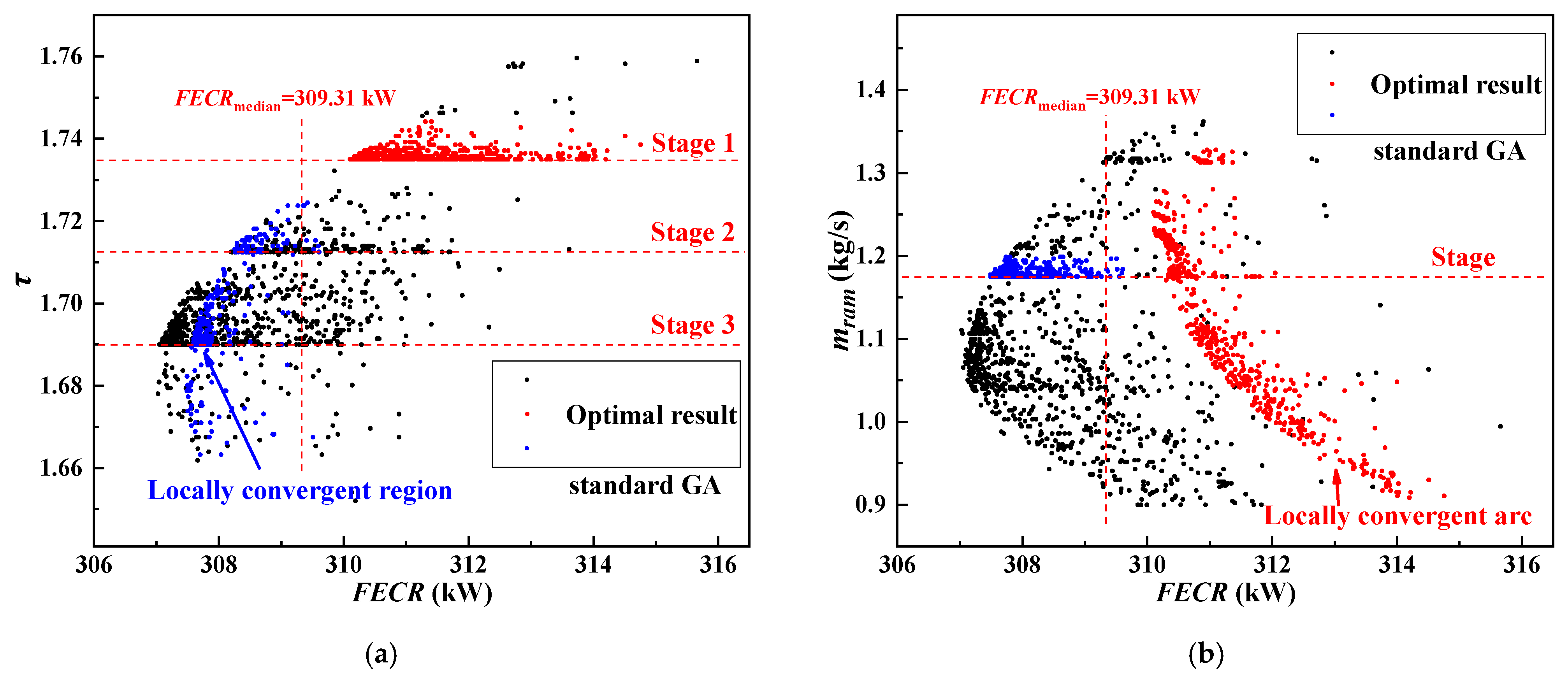
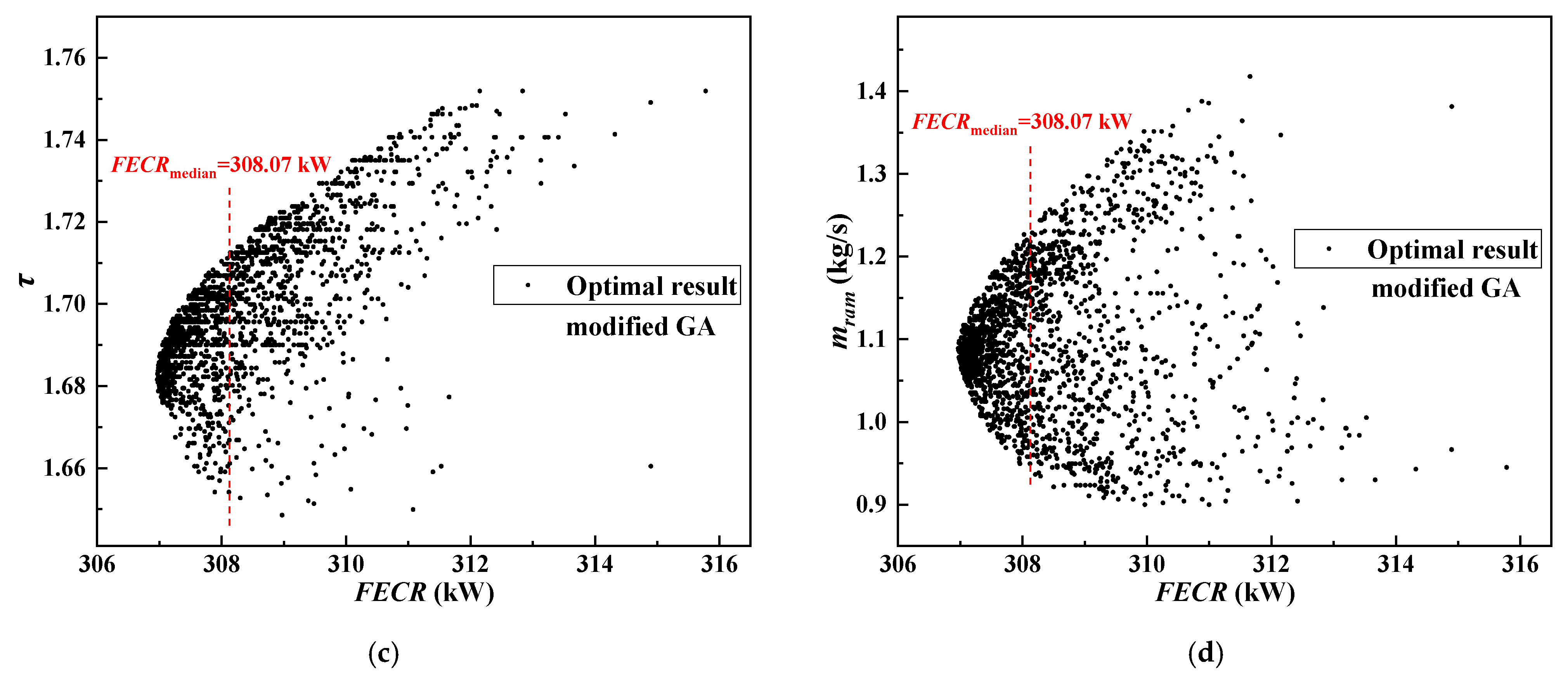
3.1. Comparison with Standard GA

To compare standard GA and modified GA, 2000 optimal results, 3000 iterations for each, are obtained from both algorithms. With standard GA, the optimal values of the defined temperature ratio τ, the ram air flow rate m_ram, and FECR are 1.678, 1.111 kg/s, and 307.03 kW, respectively. Such values obtained by modified GA are 1.682, 1.089 kg/s, and 306.97 kW. Although the difference seems not significant, it occurs only when the optimization iterations are sufficiently enough.

The optimized τ and m_ram versus FECR from the standard GA are shown in Figure 4a,b. There are three evident locally convergent stages for the temperature ratio at the value of 1.69, 1.7125, and 1.735. The corresponding binary strings are 10000000, 10100000, and 11000000. Similarly, there is also a locally convergent stage for the ram air flow rate occurring at 1.175 kg/s with the binary string of 10000000. As mentioned in the previous part, such binary string is hard to change to an adjacent one through a single mutation step, which is the leading cause of the local convergence. Furthermore, the independent optimization variables influence each other, which is also due to the discontinuity in mutation. As shown in Figure 4a,b, the locally convergent (stage 1) in the temperature ratio of 1.735 maps a locally convergent arc (red points) in the ram air flow rate. Similarly, another locally convergent region (blue points) in the Figure τ-FECR is caused by the locally convergent stage (blue points) in the flow rate of ram air. Therefore, the global convergence property of the standard GA needs to improve.

By comparison, no apparent locally convergent region exists in the results obtained from the modified GA in Figure 4c,d. Most of the optimized data are located in the globally convergent region. Furthermore, the medians of optimal FECR by using standard and modified GA are, respectively, 309.31 kW and 308.07 kW. It indicates that the proposed modified GA effectively resolves the deficiency caused by the discontinuity when using standard GA.

A further comparison in the computational efficiency between the two algorithms can be seen in Figure 5. The above 2000 results, respectively, obtained from standard and modified GA are arranged in the order of FECR from smallest to largest. Due to the discontinuity in standard GA, only 29.3% of the optimized FECRs lower than 308 kW, while such share increases to 47.6% when using the modified GA. Furthermore, there is an apparent non-smooth point at around 310 kW in the curve obtained from the standard GA. This is caused by the locally convergent value of τ = 1.735. In contrast, the statistical results by modified GA keep continuous in the whole range. It says again that the modified GA has superiority in convergence, which speeds up the energy-saving design of ECS.

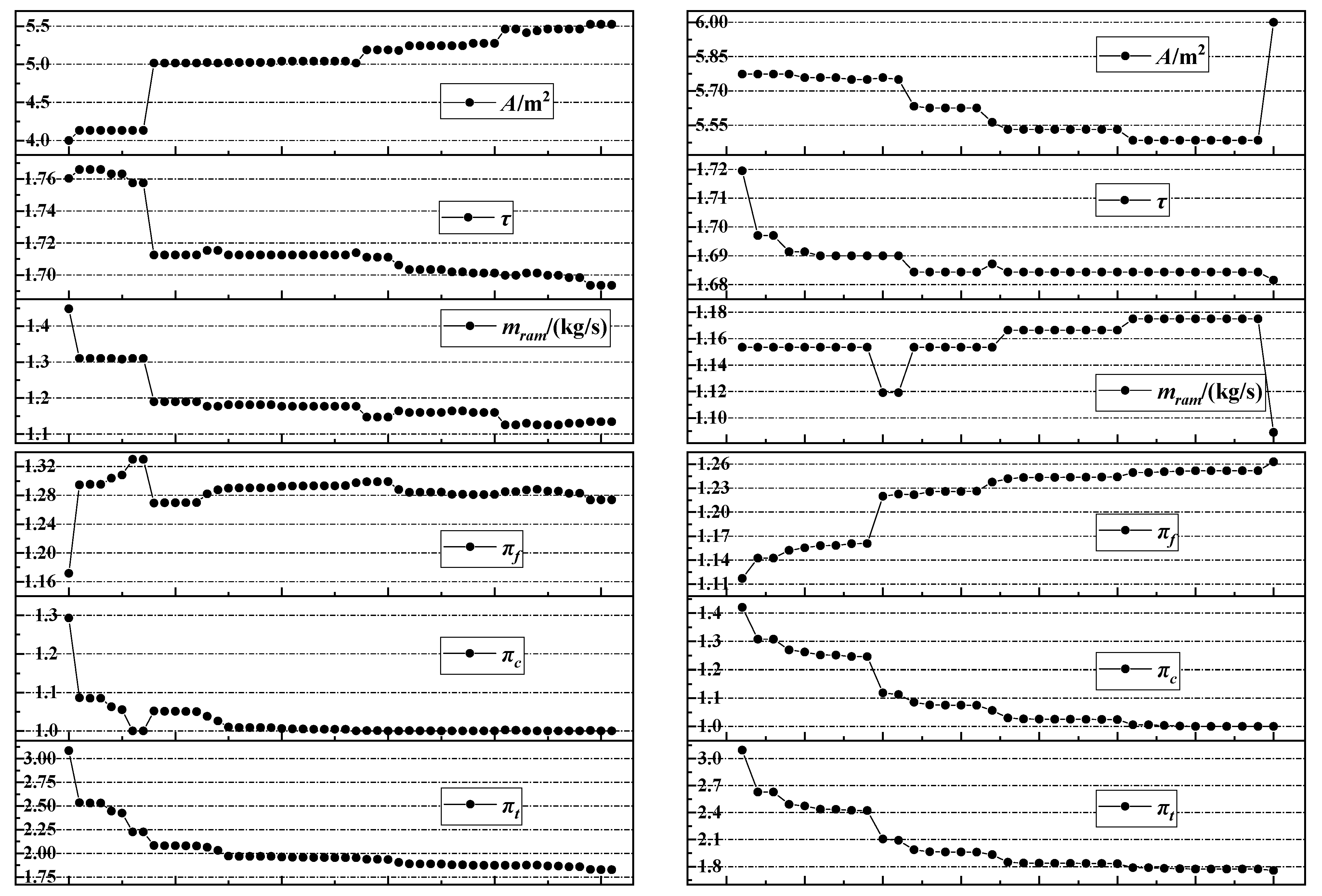
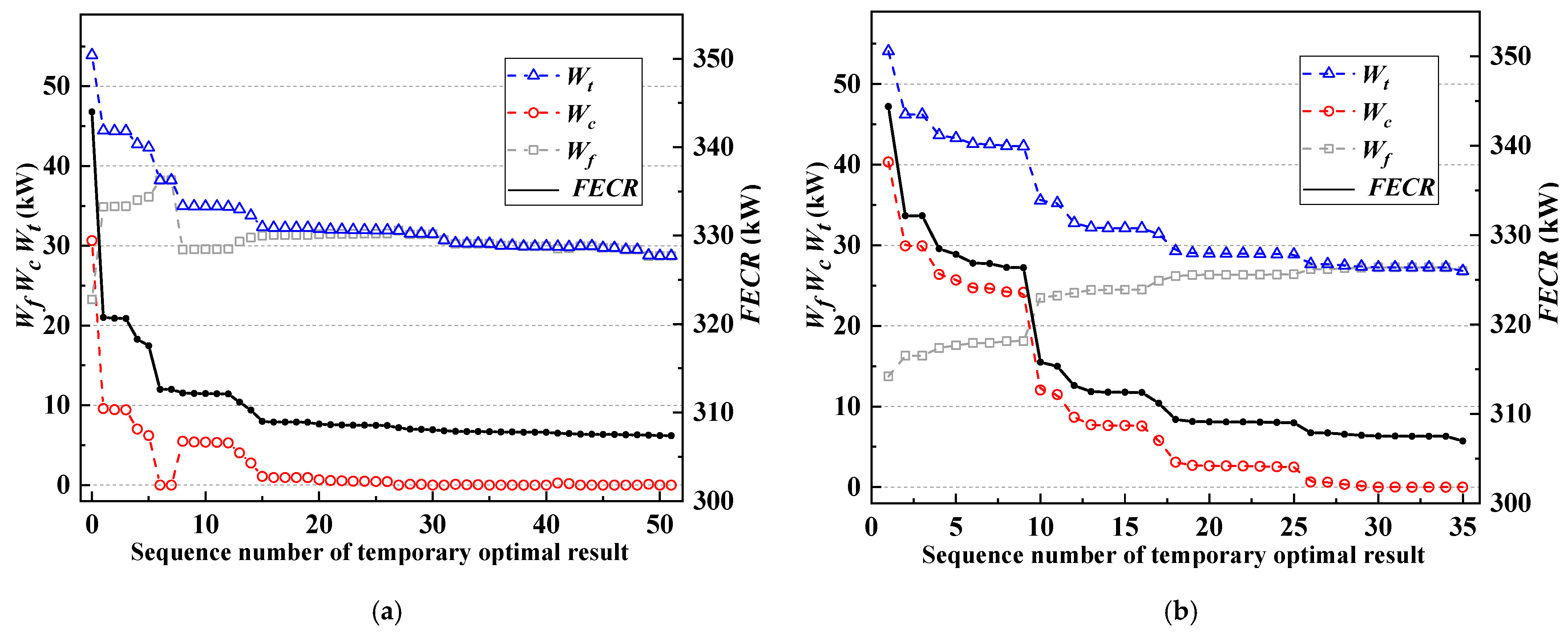
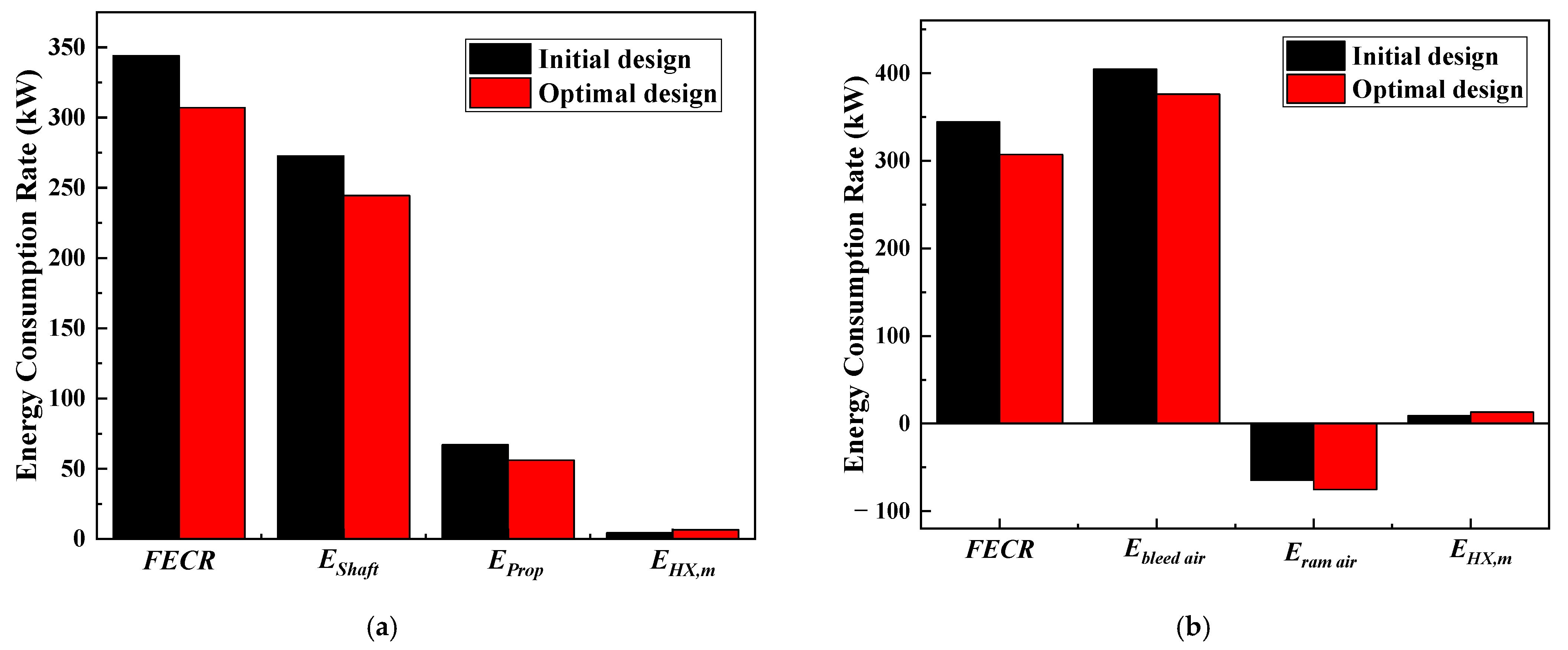
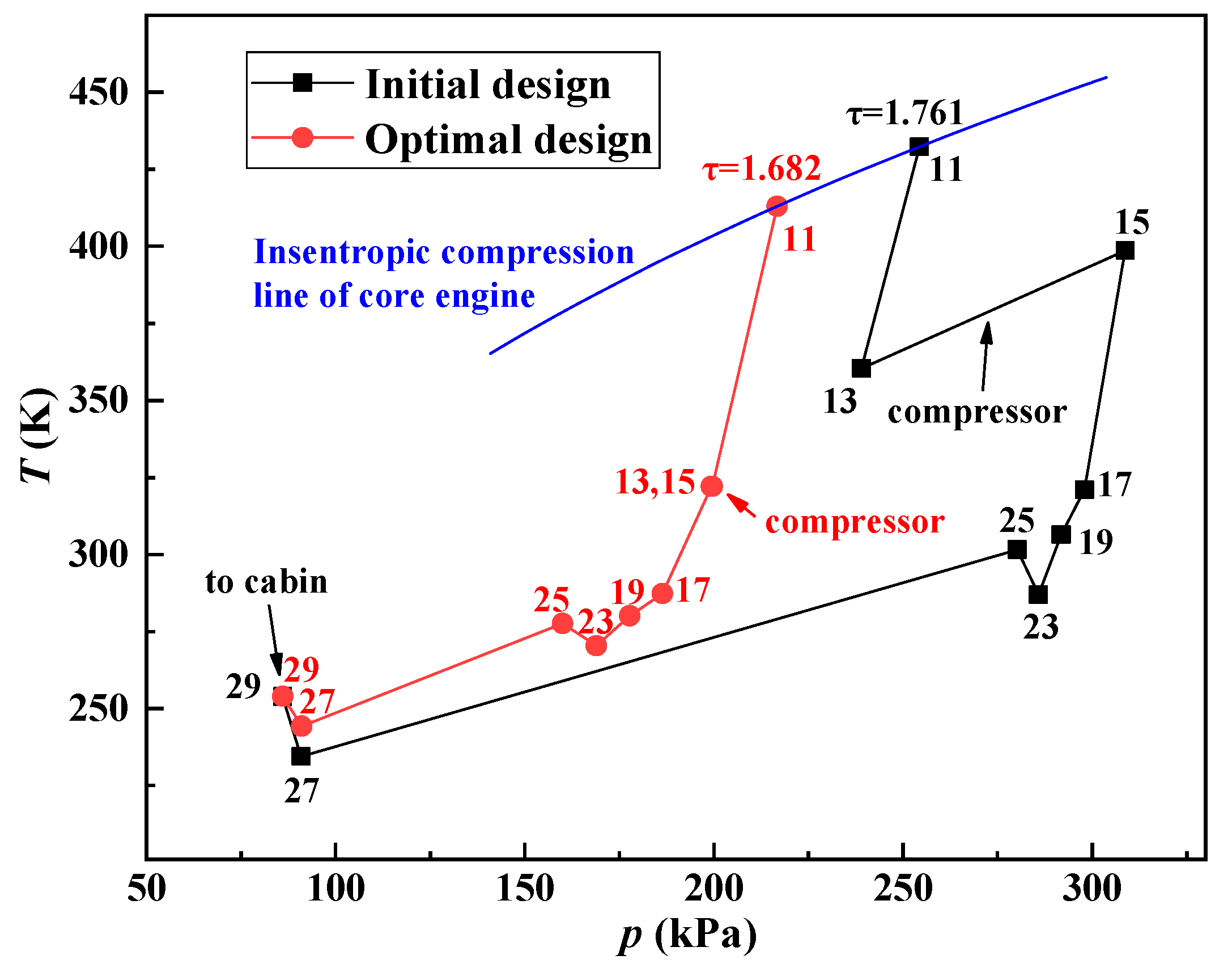
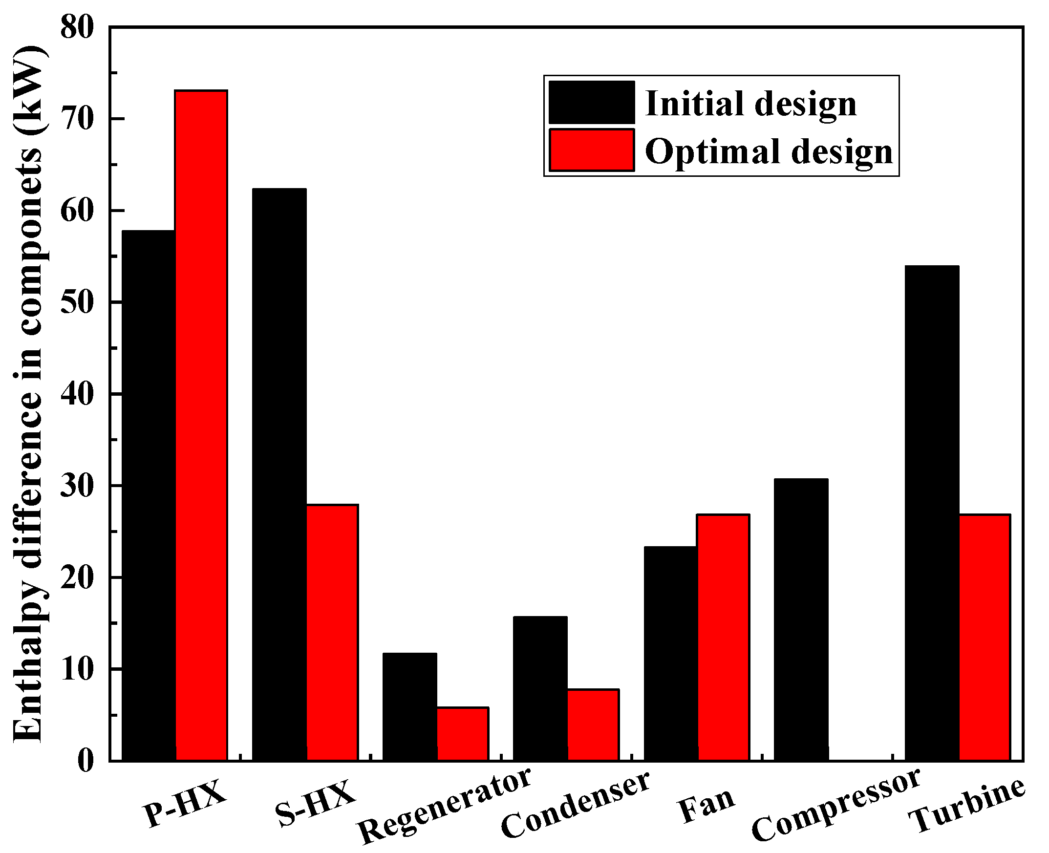
3.2. Analysis of the Optimized ECS

Compared with the initial configuration, two optimization cases obtained through the modified GA method are shown in

Table 6. Initial and optimal systematic configurations.

Parameter	A1 [m2]	A2 [m2]	τ	mram [kg/s]	FECR [kW]	Cost Saved
Initial configuration	2	2	1.761	1.45	344.79	\
The 1st optimization case	3.469	2.055	1.694	1.134	307.39	10.8%
The 2nd optimization case	3.992	2.008	1.682	1.089	306.97	11.0%

. The initial inputs in the first optimization are the values of the initial configuration, while for the second optimization, the initial inputs are set randomly within the given ranges.

The requirements of the ECS cooling capacity and its outlet pressure are 33 kW and 86 kPa, both of which come from the initial configuration. With ensuring the above outputs, the FECRs of the two optimization cases are, respectively, 307.39 kW and 306.97 kW, reduced by 10.8% and 11.0%.

Figure 6 shows the variation of the optimization parameters in the above two cases, where the total heat exchanger area A, the sum of A₁ and A₂, is analyzed. During optimization, only when a new optimal result is reached in a certain iteration can it be recorded as the temporary optimal result. As shown in Figure 6, there are, respectively, 51 and 35 groups of temporary optimal results in two optimization cases.

Figure 6a shows the first optimization process using the initial configuration as the inputs. It can be found that each parameter indicates a monotone change from 1st to 7th iteration (0th point refers to the initial configuration). Among them, the trends of τ, π_c, π_t, E_Shaft are decline, and the π_f increases. Especially, π_c decreases from 1.086 to 1.000. It removes the power input for the compressor that makes the decrease of FECR from 320.7 kW to 312.6 kW. In addition, A, τ and m_ram vary gently until the 7th iteration, and the changes are all lower than 2% of the initial values.

When it continues from the 7th to the 8th iteration, all the selected variables have relatively large variations, directly moving to another searching space far from that of the 1st to 7th iteration. Due to the drastic change of A, τ, and m_ram, π_c increases from 1.0 to 1.052, while π_t continues to decrease from 2.23 to 2.08. The decrease of the turbine power output and the increase of the compression power led to a reduction of the fan power, hindering the propulsion. It causes E_Prop to experience a significant increase from 36.41 kW to 51.18 kW. Nevertheless, due to the reduction of τ, E_Shaft decreases from 271.7 kW to 255.6 kW. Even the opposite changes of E_Prop and E_Shaft make the FECR remain almost unchanged, the significant variations of variables acquire the searching area out of the locally convergent area of the first seven iterations, closer to the global optimum.

From the 8th to the last iteration, the changes of optimized design variables are all in small ranges to deeply search for the global optimum. In this stage, π_c keeps decreasing and reaches 1.0 at the 30th iteration, which is the principal reason for the decrease of FECR. Furthermore, the temperature ratio τ keeps almost unchanged from the 8th to 30th iteration. The decreasing π_c and constant τ together bring the decrease of E_Prop. Then, π_t changes from 1.94 to 1.83 with τ from 1.711 to 1.693, resulting in a further reduction of 0.66 kW in FECR to approach the global optimum.

The second optimization process with random values as the inputs is shown in Figure 6b. It can be detected that the change of FECR is positively related to π_c and π_t. A and m_ram vary drastically in the last iteration, but FECR is only decreased from 307.50 kW to 306.97 kW. It proves A and m_ram are coupled to each other, meaning that a series of combinations of them could achieve satisfactory optimization results. Moreover, π_f and E_Prop both have almost the opposite developing trends in Figure 6a,b, but they still converge to the same values. It indicates that the convergence of the modified GA is independent of the initial values.

Figure 7 shows the variations of W_f, W_c, and W_t during the optimization. Along with the decrease of π_c to 1.0 in two cases, the optimized W_c decreases to 0 kW in the end. As such, W_f and W_t finally reach an equal level. The changes in the compressor power consumption and the objective function of FECR are highly interrelated. Even after W_c is optimized to 0 kW, the small change of W_t helps the continuous decrease of FECR. It can be concluded that the turbine power inclines to be allocated more to the fan and less to the compressor during the optimization of searching for the lowest FECR. In fact, the three-wheel ECS under analysis becomes two-wheel simple type when the turbine power is used to drive the fan, whereas it becomes a two-wheel bootstrap type when driving the compressor. Therefore, from the perspective of the thermo-economics, the two-wheel simple type shows the best performance, the second is the three-wheel type worse, the two-wheel bootstrap type is the worst.

From another angle, Figure 8a shows that the energy consumptions of shaft power and propulsive power decrease sharply after optimization at the cost of a slight increase of 2.18 kW in the energy consumption of the heat exchanger weight. As a result, FECR is decreased to lower the cost of the environmental control system. In summary, there are two main reasons: (1) the decrease of τ results in the decrease of E_Shaft; (2) although the decrease of τ also lowers the turbine power, all the turbine power is used to drive the fan to save E_Prop. Figure 8b gives the energy consumptions sorted by airstreams. The energy consumption of the ram air is negative. It means that the ram air provides a propulsive work with the inputted energy from the heat exchangers and the fan. After optimization, the energy is saved in both the bleed air and ram air.

The thermodynamic cycle temperature-pressure diagrams of the initial and optimized cases are given in Figure 9, where the numbers are the corresponding nodes illustrated in Figure 1. The blue curve represents the isentropic compression process of the core engine, and any point in this curve can be chosen as the supply point of the bleed air. On the whole, the temperature and pressure in the thermodynamic process of the optimized ECS keep almost decreasing and finally reach the same point as the initial one. We can find that the optimized cycle differs from the initial one mainly in two aspects. The first one is the air entrance position. In the optimized cycle, the inlet pressure of the bleed air is lower, meaning lower shaft power demand from the main engine. The second one is the compression process from node 13 to 15. As mentioned above, the compression process is eliminated in the optimized cycle. It brings more power input to the fan which saves the propulsive power consumed by the ram air. Due to the decrease of inlet parameters of bleed air and the elimination of compression, the optimized ECS saves 11.0% of the total energy consumption. Figure 10 presents the enthalpy differences in the ECS components to show the energy conversion process. The results are compared before and after optimization. The sum of heat exchange in the primary HX and the secondary HX decreases because of the decline of the ram air mass flow. The heat exchanges in the heat regenerator and condenser are nearly halved, which is affected by the decline in the turbine work. The two different energy conversion processes lead to the same output, while the energy consumption has been saved by the optimal design.

4. Conclusions

In this paper, the optimal design of the aircraft ECS is conducted by coupling the component-level models and the modified GA. To reach a better design of ECS with lower power consumption, several key design variables are optimized to obtain the system configuration of minimum FECR. The major conclusions are drawn as follows:

(1) A novel evaluation method of energy utilization for ECS is proposed. The system output is set constant to avoid its unquantifiable characteristic with a thermo-economics criterion of FECR to evaluate the total energy consumption. In FECR, different forms of energy, including shaft power and propulsive power, are summed up with the weighting coefficient determined by the energy quality.

(2) The continuity improvement implemented in the modified GA makes it have a better convergence. Compared with 29.3% of the optimized FECR lower than 308 kW by using standard GA, the modified GA increases such share to 47.6%, and the growth rate is up to 62.4%. This modification on the algorithm improves the efficiency of energy-saving optimization of such energy systems such as ECS.

(3) The areas of two heat exchangers, the bleed air temperature ratio and the mass flow rate of the ram air are selected as the design variables to be optimized. The pressure ratios of the fan, compressor and turbine in ECS also vary to ensure the outputs meet the demand. After optimization, the FECR decreases from 344.79 kW to 306.97 kW, cutting the energy consumption by 11.0%.

(4) Due to the decrease of inlet parameters of bleed air and the elimination of power input in the compressor, both the shaft power input and the propulsive power consumption can be reduced effectively. These are the main reasons for the decreased energy consumption of the optimized ECS.

References

1. Fawal, S.; Kodal, A. Comparative performance analysis of various optimization functions for an irreversible Brayton cycle applicable to turbojet engines. Energy Convers. Manag. 2019, 199, 111976.1–111976.13. [Google Scholar] [CrossRef]
2. Tuzcu, H.; Sohret, Y.; Caliskan, H. Energy, environment and enviroeconomic analyses and assessments of the turbofan engine used in aviation industry. Environ. Prog. Sustain. Energy 2021, 40, e13547. [Google Scholar] [CrossRef]
3. Aygun, H.; Turan, O. Exergetic sustainability off-design analysis of variable-cycle aero-engine in various bypass modes. Energy 2020, 195, 117008. [Google Scholar] [CrossRef]
4. Dechow, M.; Nurcombe, C. Aircraft environmental control systems. In Air Quality in Airplane Cabins and Similar Enclosed Spaces; Springer: Berlin/Heidelberg, Germany, 2005. [Google Scholar]
5. Linnett, K.; Crabtree, R. What’s next in commercial aircraft environmental control systems? SAE Trans. 1993, 102, 639–653. [Google Scholar]
6. He, H.; Hao, J. Optimum design for environmental control system of aircraft cabin. J. Beijing Univ. Aeronaut. Astronaut. 1996, 5, 55–61. [Google Scholar]
7. Hong, W.; Wang, J. Aircraft ECS reliability design and evaluation. Acta Aeronaut. ET Astronaut. Sin. 1998, 02, 97–100. [Google Scholar]
8. Ma, J.; Chen, L.; Liu, H. Fault diagnosis for the heat exchanger of the aircraft environmental control system based on the strong tracking filter. PLoS ONE 2015, 10, e0122829. [Google Scholar] [CrossRef]
9. Li, H.B.; Dong, X.M.; Guo, J.; Chen, Y.; Li, T.T. Heat exchanger optimization analysis of aircraft environmental control system. Adv. Mater. Res. 2011, 383–390, 5536–5541. [Google Scholar] [CrossRef]
10. Vargas, J.V.C.; Bejan, A. Thermodynamic optimization of finned crossflow heat exchangers for aircraft environmental control systems. Int. J. Heat Fluid Flow 2001, 22, 657–665. [Google Scholar] [CrossRef]
11. Alebrahim, A.; Bejan, A. Thermodynamic optimization of heat-transfer equipment configuration in an environmental control system. Int. J. Energy Res. 2001, 25, 1127–1150. [Google Scholar] [CrossRef]
12. Ordonez, J.C.; Bejan, A. Minimum power requirement for environmental control of aircraft. Energy 2003, 28, 1183–1202. [Google Scholar] [CrossRef]
13. Pérez-Grande, I.; Leo, T.J. Optimization of a commercial aircraft environmental control system. Appl. Therm. Eng. 2002, 22, 1885–1904. [Google Scholar] [CrossRef]
14. Vargas, J.; Bejan, A. Integrative thermodynamic optimization of the environmental control system of an aircraft. Int. J. Heat Mass Transf. 2001, 44, 3907–3917. [Google Scholar] [CrossRef]
15. Yoo, Y.J.; Lee, H.J.; Kho, S.H.; Ki, J.Y. A study on modeling program development of an environmental control system. J. Korean Soc. Propuls. Eng. 2009, 13, 57–63. [Google Scholar]
16. Bello-Ochende, T.; Simasiku, E.; Baloyi, J. Optimum design of heat exchanger for environmental control system of an aircraft using entropy generation minimization (EGM) technique. In Proceedings of the 12th International Conference on Heat Transfer, Fluid Mechanics and Thermodynamics, Malaga, Spain, 11–13 July 2016. [Google Scholar]
17. Tipton, R.; Figliola, R.S.; Ochterbeck, J.M. Thermal optimization of the ECS on an advanced aircraft with an emphasis on system efficiency and design methodology. In Proceedings of the SAE Aerospace Power Systems Conference & Exposition, Warrendale, PA, USA, 4 April 1997; SAE International: Warrendale, PA, USA, 1997. [Google Scholar]
18. Figliola, R.S.; Tipton, R.; Li, H. Exergy approach to decision-based design of integrated aircraft thermal systems: Exergy. J. Aircr. 2003, 40, 49–55. [Google Scholar] [CrossRef]
19. Zhao, H.; Yu, H.; Zhu, Y.; Chen, L.; Chen, S. Experimental study on the performance of an aircraft environmental control system. Appl. Therm. Eng. 2009, 29, 3284–3288. [Google Scholar] [CrossRef]
20. Li, X.; Chen, Q.; Hao, J.-H.; Chen, X.; He, K.-L. Heat current method for analysis and optimization of a refrigeration system for aircraft environmental control system. Int. J. Refrig. 2019, 106, 163–180. [Google Scholar] [CrossRef]
21. Cui, G.W. The Research on Optimization Method of Aircraft Environment Control System. Master’s Thesis, Nanjing University of Aeronautics and Astronautics, Nanjing, China, December 2010. [Google Scholar]
22. Tu, Y.; Lin, G.P. Dynamic simulation of aircraft environmental control system based on flowmaster. J. Aircr. 2011, 48, 2031–2041. [Google Scholar] [CrossRef]
23. Bejan, A.; David, L.S. The need for exergy analysis and thermodynamic optimization in aircraft development. Exergy Int. J. 2001, 1, 14–24. [Google Scholar] [CrossRef]
24. Hou, X.D. The Simulation and Research of Aircraft Environment Control System. Master’s Thesis, Nanjing University of Aeronautics and Astronautics, Nanjing, China, December 2010. [Google Scholar]
25. Jiang, H.; Dong, S.; Zhang, H. Energy efficiency analysis of electric and conventional environmental control system on commercial aircraft. In Proceedings of the 2016 IEEE/CSAA International Conference on Aircraft Utility Systems(AUS), Beijing, China, 10–12 October 2016. [Google Scholar]
26. Yang, Y.; Gao, Z. Power optimization of the environmental control system for the civil more electric aircraft. Energy 2019, 172, 196–206. [Google Scholar] [CrossRef]
27. Dai, Y.; Wang, J.; Lin, G. Exergy analysis, parametric analysis and optimization for a novel combined power and ejector refrigeration cycle. Appl. Therm. Eng. 2009, 29, 1983–1990. [Google Scholar] [CrossRef]
28. Zhang, S.; Wang, H.; Tao, G. Performance comparison and parametric optimization of subcritical organic rankine cycle (ORC) and transcritical power cycle system for low-temperature geothermal power generation. Appl. Energy 2011, 88, 2740–2754. [Google Scholar]
29. Perera, A.; Attalage, R.A.; Perera, K.; Dassanayake, V. A hybrid tool to combine multi-objective optimization and multi-criterion decision making in designing standalone hybrid energy systems. Appl. Energy 2013, 107, 412–425. [Google Scholar] [CrossRef]
30. Shiba, T.; Bejan, A. Thermodynamic optimization of geometric structure in the counterflow heat exchanger for an environmental control system. Energy 2001, 26, 493–512. [Google Scholar] [CrossRef]
31. Sanaye, S.; Hajabdollahi, H. Thermal-economic multi-objective optimization of plate fin heat exchanger using genetic algorithm. Appl. Energy 2010, 87, 1893–1902. [Google Scholar] [CrossRef]
32. Bejan, A. A role for exergy analysis and optimization in aircraft energy-system design. In Proceedings of the ASME International Mechanical Engineering Congress and Exposition, Nashville, TN, USA, 14–19 November 1999. [Google Scholar]
33. Mishra, M.; Das, P.K.; Sarangi, S. Second law based optimisation of crossflow plate-fin heat exchanger design using genetic algorithm. Appl. Therm. Eng. 2009, 29, 2983–2989. [Google Scholar] [CrossRef] [Green Version]
34. Patel, V.; Rao, R. Design optimization of shell-and-tube heat exchanger using particle swarm optimization technique. Appl. Therm. Eng. 2010, 30, 1417–1425. [Google Scholar] [CrossRef]
35. West, A.; Sherif, S. Optimization of multistage vapour compression systems using genetic algorithms. Part 1: Vapour compression system model. Int. J. Energy Res. 2001, 25, 803–812. [Google Scholar] [CrossRef]
36. Mo, Z.J.; Zhu, X.J.; Wei, L.Y.; Cao, G.Y. Parameter optimization for a pemfc model with a hybrid genetic algorithm. Int. J. Energy Res. 2006, 30, 585–597. [Google Scholar] [CrossRef]
37. Avval, H.B.; Ahmadi, P.; Ghaffarizadeh, A.R.; Saidi, M.H. Thermo-economic-environmental multiobjective optimization of a gas turbine power plant with preheater using evolutionary algorithm. Int. J. Energy Res. 2011, 35, 389–403. [Google Scholar] [CrossRef]
38. Özçelik, Y. Exergetic optimization of shell and tube heat exchangers using a genetic based algorithm. Appl. Therm. Eng. 2007, 27, 1849–1856. [Google Scholar] [CrossRef]
39. Valdevit, L.; Pantano, A.; Stone, H.A.; Evans, A.G. Optimal active cooling performance of metallic sandwich panels with prismatic cores. Int. J. Heat Mass Transf. 2006, 49, 3819–3830. [Google Scholar] [CrossRef]
40. Guan, B.; Zhang, C.; Ning, J. Genetic algorithm with a crossover elitist preservation mechanism for protein–ligand docking. Amb Express 2017, 7, 174. [Google Scholar] [CrossRef] [PubMed] [Green Version]
41. Peng, H.; Ling, X. Optimal design approach for the plate-fin heat exchangers using neural networks cooperated with genetic algorithms. Appl. Therm. Eng. 2008, 28, 642–650. [Google Scholar] [CrossRef]
42. Maser, A.; Garcia, E.; Mavris, D. Characterization of thermodynamic irreversibility for integrated propulsion and thermal management systems design. In Proceedings of the 50th AIAA Aerospace Sciences Meeting including the New Horizons Forum and Aerospace Exposition, Nashville, TN, USA, 9–12 January 2012; p. 1124. [Google Scholar]
43. “Type-Certificate Data Sheet RB211 Trent 700 Series Engines” (PDF). EASA. 14 October 2014. Archived from the Original (PDF) on 16 August 2016. Retrieved 1 July 2017. Available online: https://www.easa.europa.eu/document-library/type-certificates/engine-cs-e/easae042-rolls-royce-deutschland-rb211-trent-700 (accessed on 14 March 2022).
44. Guo, J.; Cheng, L.; Xu, M. Optimization design of shell-and-tube heat exchanger by entropy generation minimization and genetic algorithm. Appl. Therm. Eng. 2009, 29, 2954–2960. [Google Scholar] [CrossRef]
Figure 1. Schematic diagram of ECS.
Processes 10 00721 g001
Figure 2. Multipoint crossover process.
Processes 10 00721 g002
Figure 3. Calculating flowchart of ECS optimization using GA.
Processes 10 00721 g003
Figure 4. Distributions of design variables with the corresponding optimal FECR. (a) 2000 optimal results over 3000 iterations of standard GA, τ-FECR; (b) 2000 optimal results over 3000 iterations of standard GA, mram-FECR; (c) 2000 optimal results over 3000 iterations of modified GA, τ-FECR; (d) 2000 optimal results over 3000 iterations of modified GA, mram-FECR.
Processes 10 00721 g004aProcesses 10 00721 g004b
Figure 5. Comparison between the modified GA and standard GA.
Processes 10 00721 g005
Figure 6. Variation of ECS parameters during optimization. (a) Optimization process of the 1st optimal result; (b) Optimization process of the 2nd optimal result.
Processes 10 00721 g006aProcesses 10 00721 g006b
Figure 7. Variation of fan power, compressor power, and turbine power. (a) Optimization process of the 1st optimal result; (b) Optimization process of the 2nd optimal result.
Processes 10 00721 g007
Figure 8. Comparison of energy consumptions. (a) sorted by energy form; (b) sorted by airstreams.
Processes 10 00721 g008
Figure 9. Thermodynamic cycle of the bleed air.
Processes 10 00721 g009
Figure 10. Enthalpy differences in ECS components.
Processes 10 00721 g010