
Application of Intelligent Control in Chromatography Separation Process


Abstract
:1. Introduction
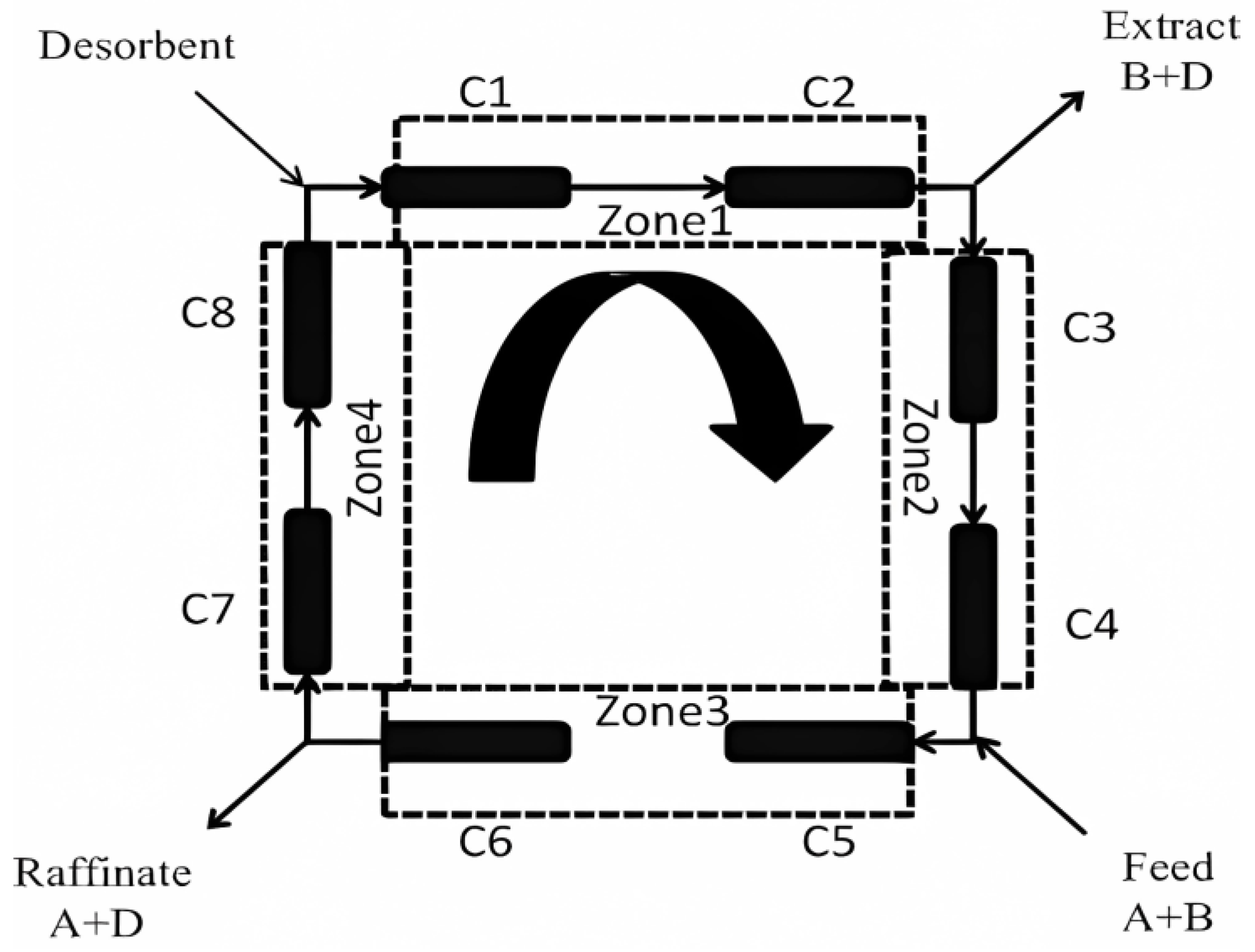
2. SMB Mathematical Discrete Model
2.1. TMB and SMB Equation Model
2.2. SMB Digitization via Crank–Nicolson Method
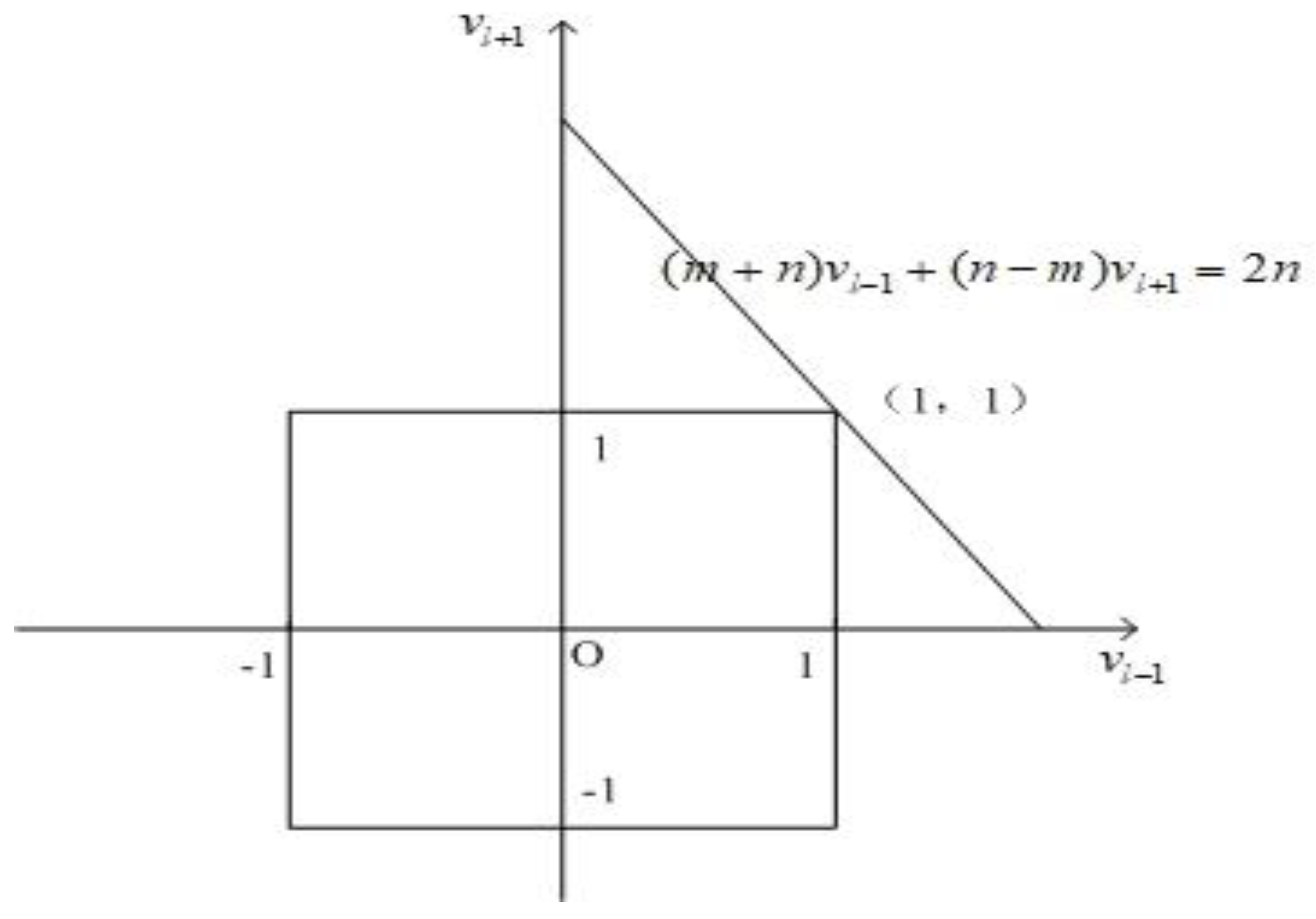
2.3. Stability Analysis
- (1)
- When . According to , so we can obtain the equation in component :
- (2)
- When , it means that
- (3)
- When , it means that
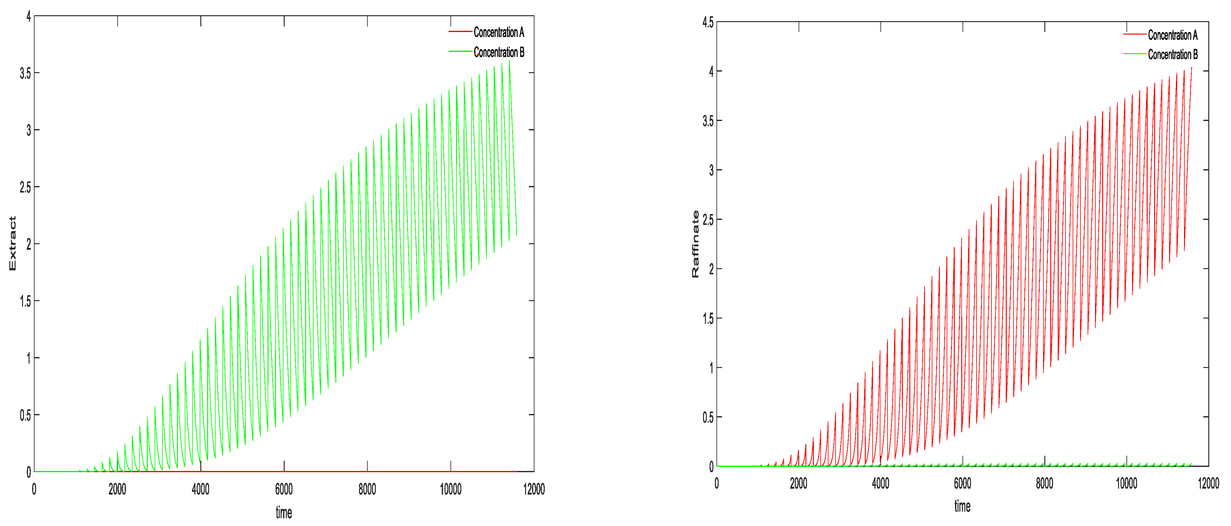
3. Simulation
3.1. Experimental Environment and Data
3.2. Sensitivity Analysis of Purity Flow Rates to Find Local Monotonic Intervals
4. Smart Controller Design
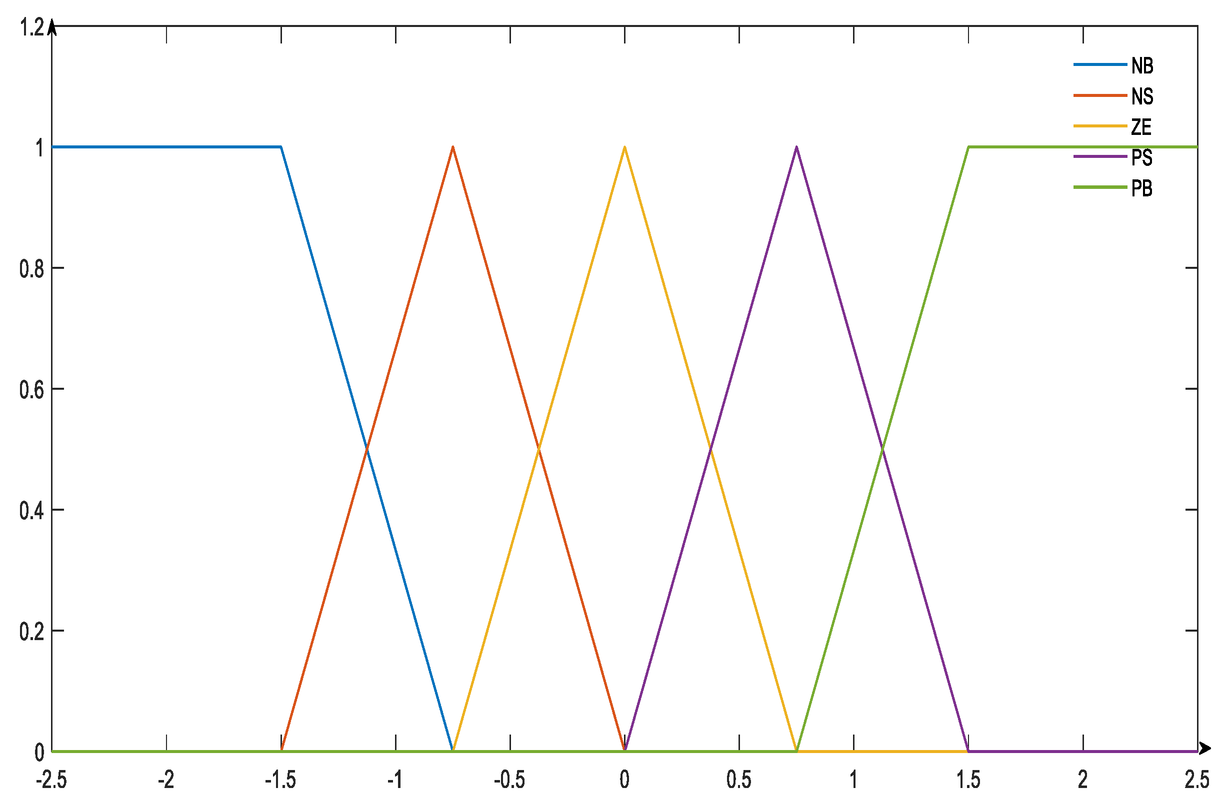
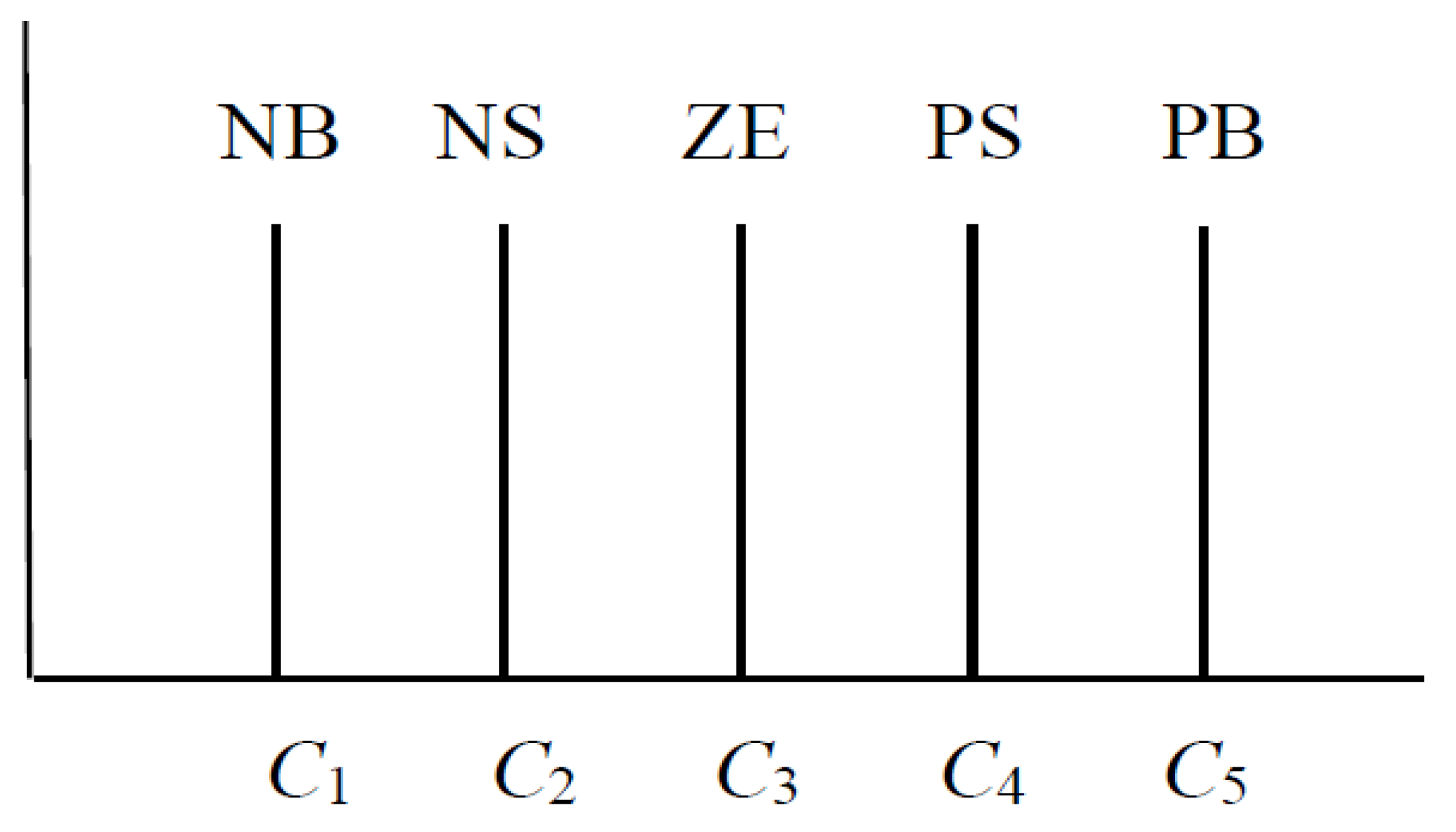
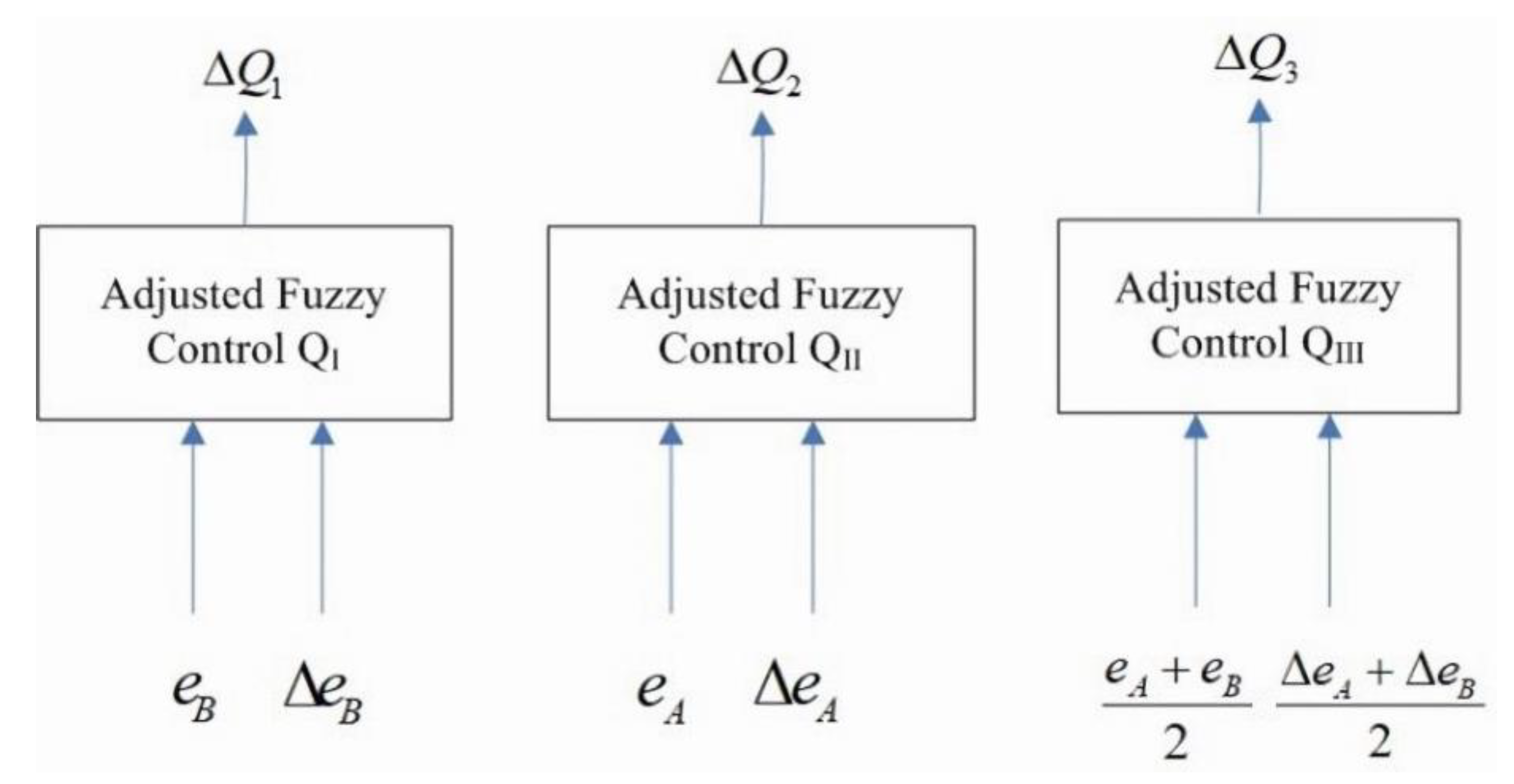
4.1. Fuzzy Rule Control and Hierarchical Design
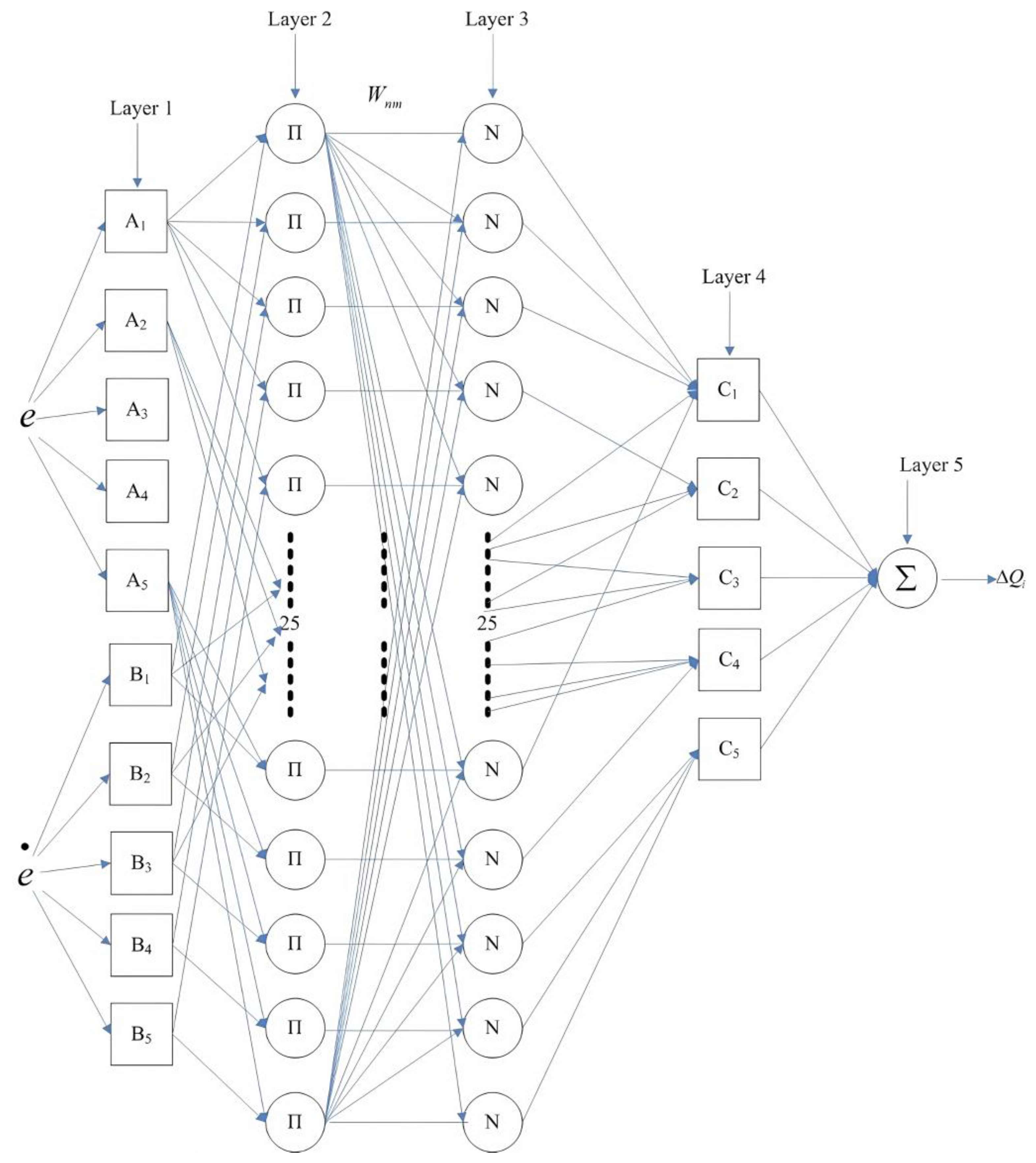
4.2. NN-like Fuzzy Controller Framework
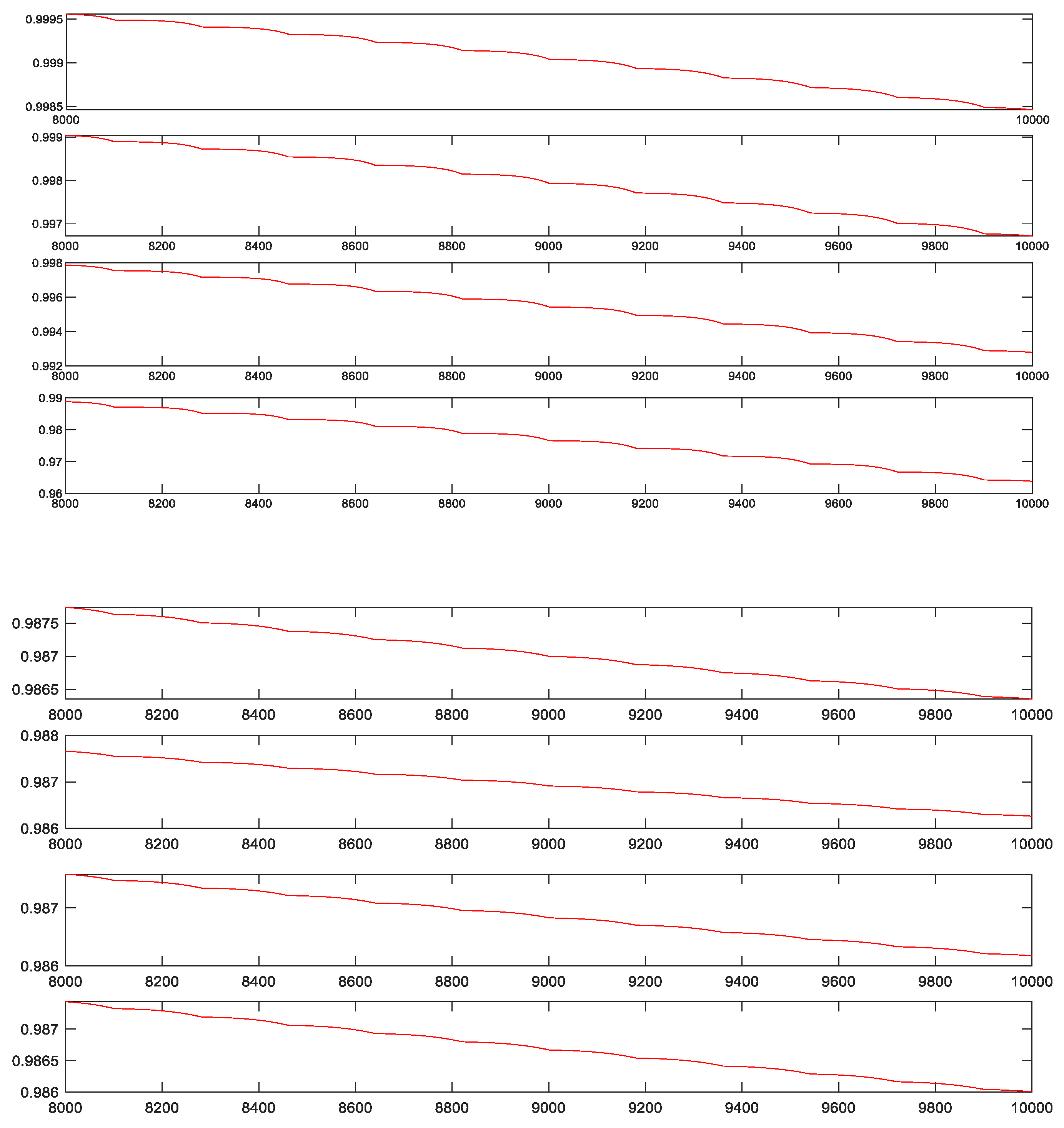
5. SMB Control Experiments
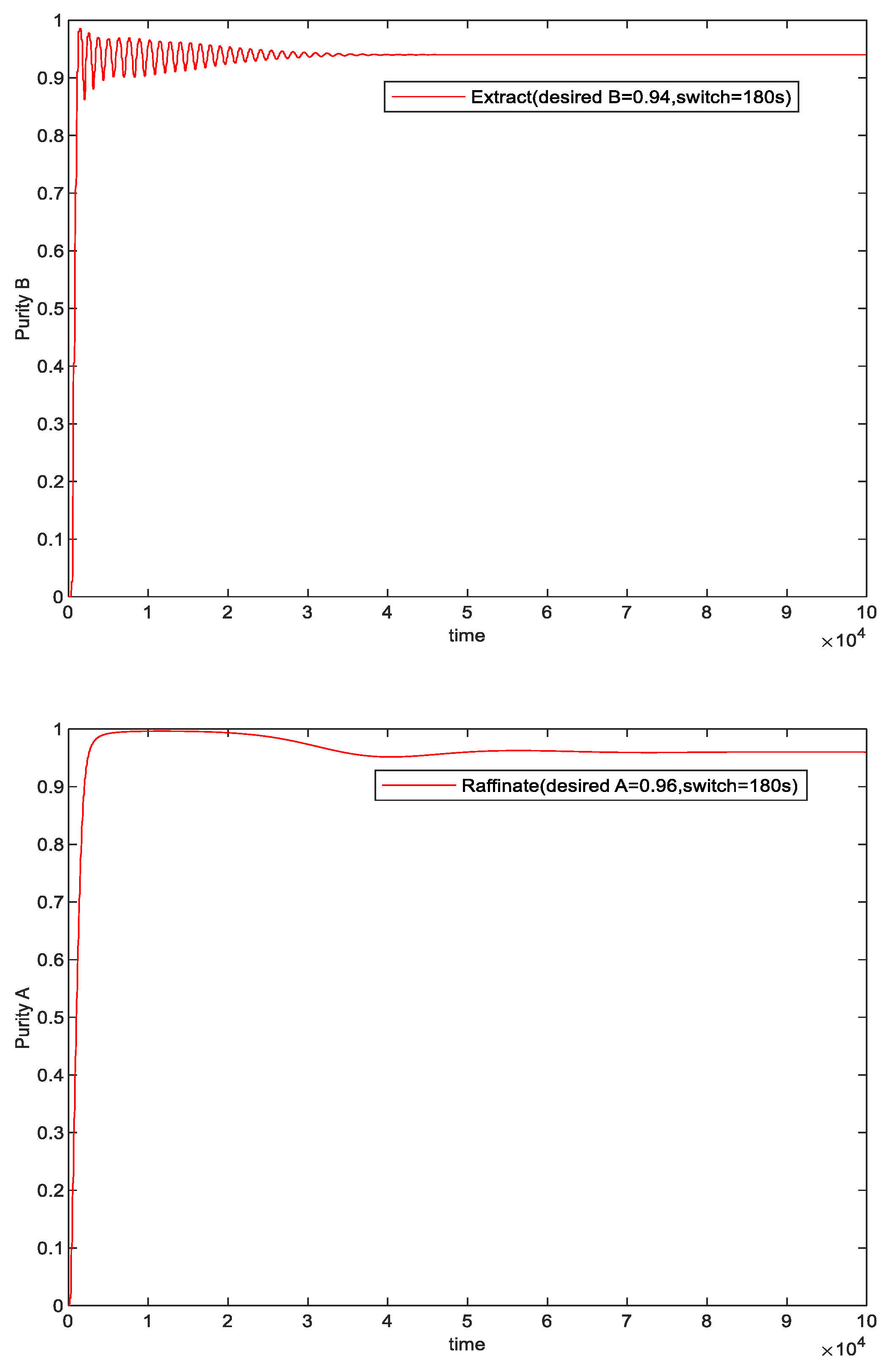
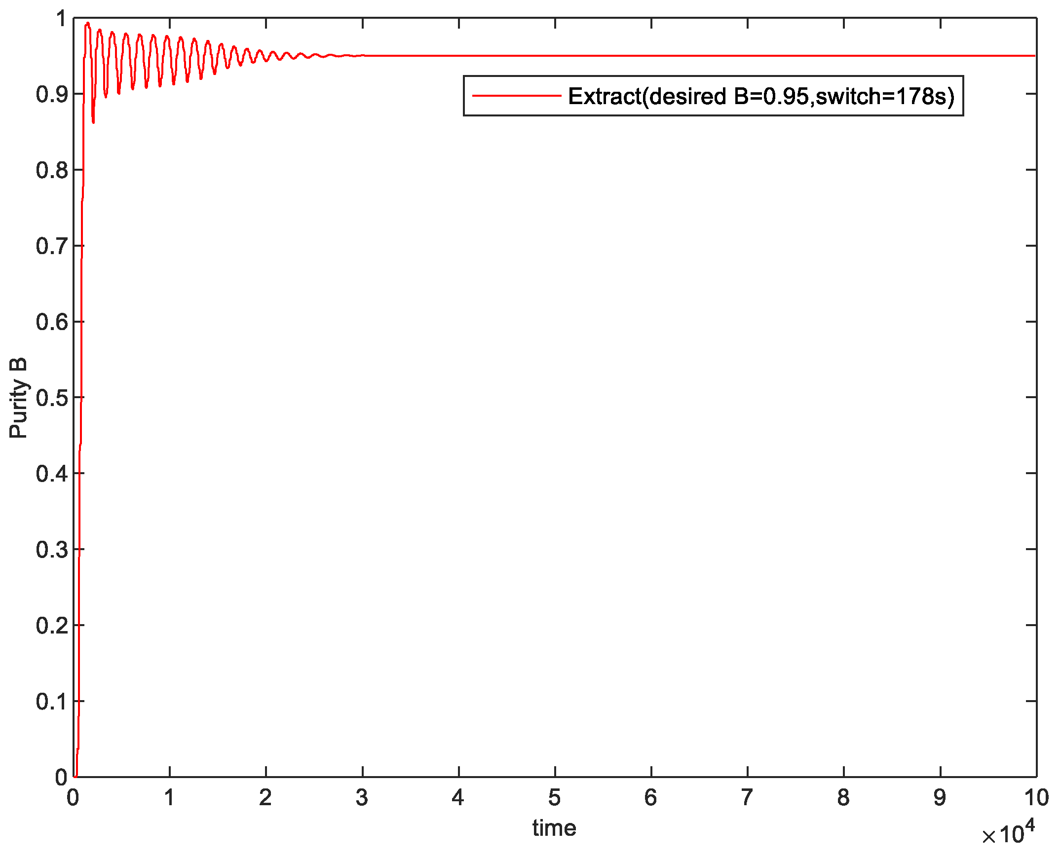
5.1. Purity Control Result
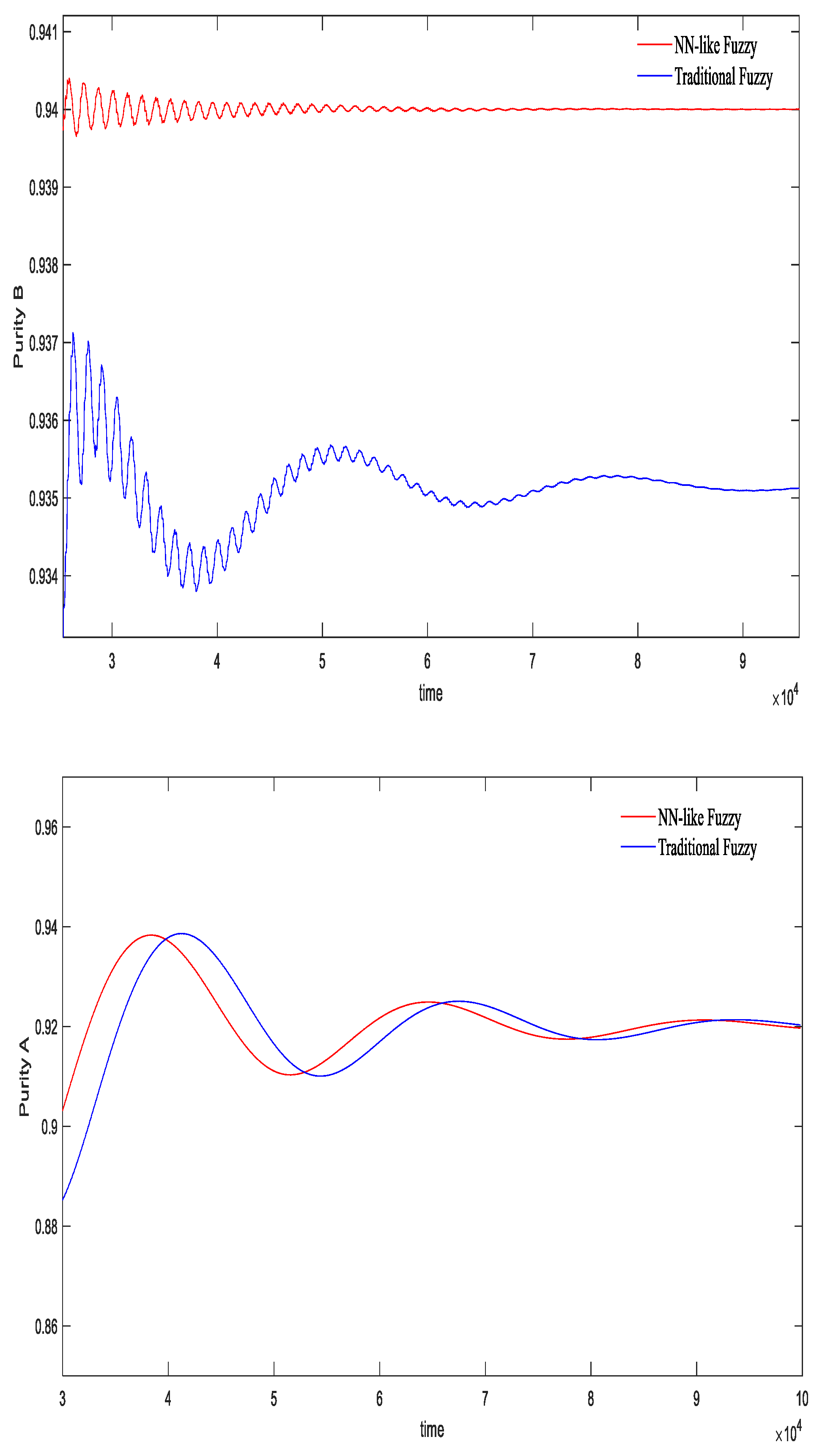
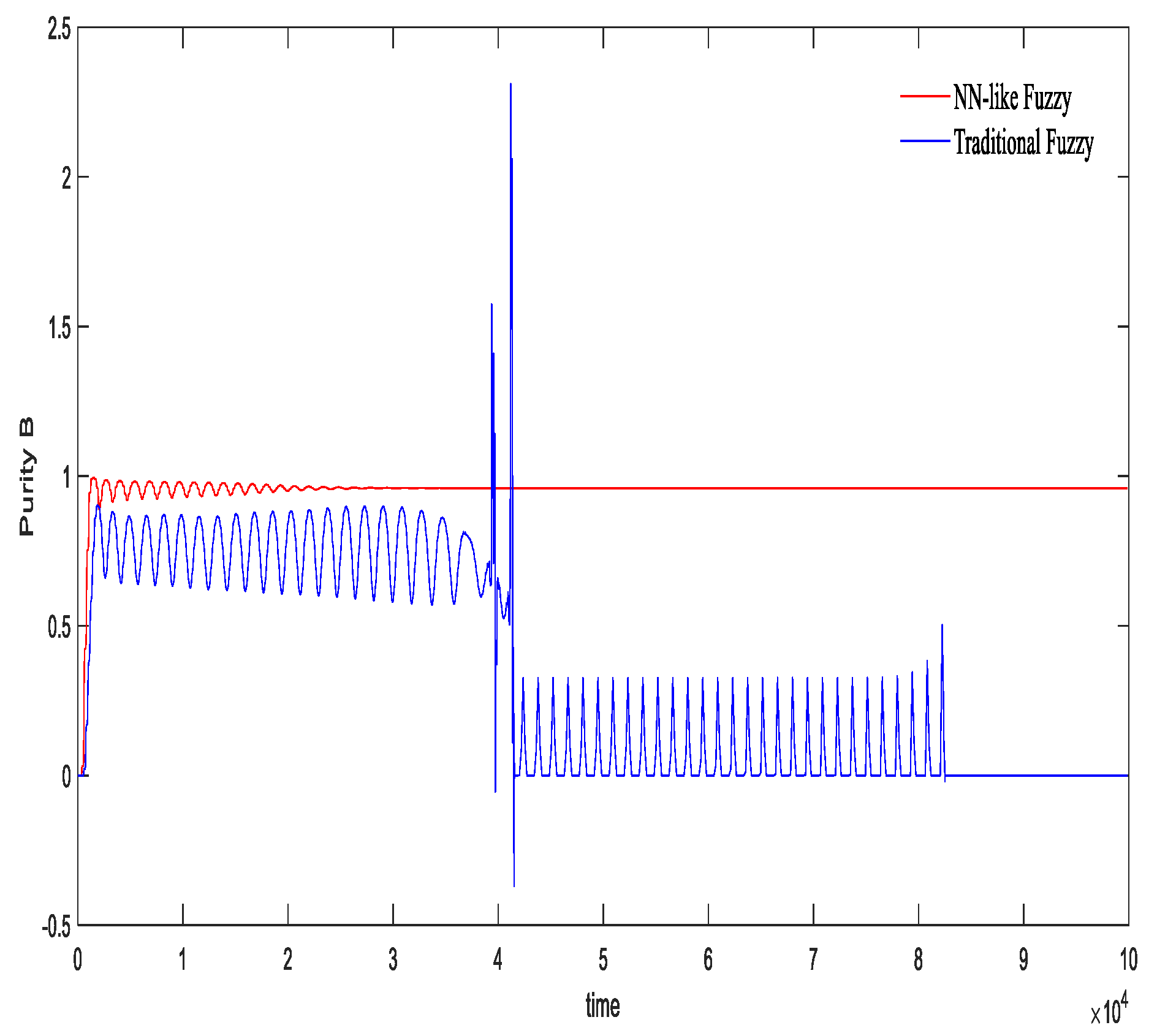
5.2. Controller Comparison
6. Discussion
7. Conclusions
Author Contributions
Funding
Data Availability Statement
Acknowledgments
Conflicts of Interest
References
- Kim, K.M.; Han, K.W.; Kim, S.I.; Bae, Y.S. Simulated moving bed with a product column for improving the separation performance. J. Ind. Eng. Chem. 2020, 88, 328–338. [Google Scholar] [CrossRef]
- Reinaldo, C.S.; Gomes, B.A.; Resende, S.A. Optimal performance comparison of the simulated moving bed process variants based on the modulation of the length of zones and the feed concentration. J. Chromatogr. A 2021, 1651, 462280. [Google Scholar] [CrossRef]
- Supelano, R.C.; Barreto, A.G., Jr.; Neto, A.S.A.; Secchi, A.R. One-step optimization strategy in the simulated moving bed process with asynchronous movement of ports: A VariCol case study. J. Chromatogr. A 2020, 1634, 1672–1718. [Google Scholar] [CrossRef]
- Li, S.; Wei, D.; Wang, J.S.; Yan, Z.; Wang, S.Y. Predictive control method of simulated moving bed chromatographic separation process based on piecewise affine. Int. J. Appl. Math. 2020, 50, 1–12. [Google Scholar]
- Gomes, P.S. Methodologies and Product (FlexSMB-LSRE) Development. Ph.D. Thesis, Faculdade de Engenharia da Universidade do Porto (FEUP), Porto, Portugal, 2009. [Google Scholar]
- Schulte, M.; Strube, J. Preparative enantioseparation by simulated moving bed chromatography. J. Chromatogr. A 2001, 906, 399–416. [Google Scholar] [CrossRef] [PubMed]
- Klatt, K.U.; Hanisch, F.; Dunnebier, G. Mode-based control of a simulated moving bed chromatographic process for the separation of frutose and glucose. J. Process Control 2002, 12, 203–219. [Google Scholar] [CrossRef]
- Neto, A.S.A.; Secchi, A.R.; Souza, M.B.; Barreto, A.G. Nonlinear model predictive control applied to the separation of praziquantel in simulated moving bed chromatography. J. Chromatogr. A 2016, 1470, 42–49. [Google Scholar] [CrossRef] [PubMed]
- Nogueira, I.B.; Rodrigues, A.E.; Loureiro, J.M.; Ribeiro, A.M. Novel Switch Stabilizing Model Predictive Control Strategy Applied in the Control of a Simulated Moving Bed for the Separation of Bi-Naphthol Enantiomers. Ind. Eng. Chem. Res. 2020, 59, 1979–1988. [Google Scholar] [CrossRef]
- Lee, J.W.; Seidel-Morgenstern, A. Model Predictive Control of Simulated Moving Bed Chromatography for Binary and Pseudo-binary Separations: Simulation Study. IFAC-PapersOnLine 2018, 51, 530–535. [Google Scholar] [CrossRef]
- Yang, Y.; Chen, X.; Zhang, N. Optimizing control of adsorption separation processes based on the improved moving asymptotes algorithm. Adsorpt. Sci. Technol. 2018, 36, 1716–1733. [Google Scholar] [CrossRef]
- Carlos, V.; Alain, V.W. Combination of multi-model predictive control and the wave theory for the control of simulated moving bed plants. J. Chem. Eng. Sci. 2011, 66, 632–641. [Google Scholar] [CrossRef]
- Suvarov, P.; Kienle, A.; Nobre, C.; Weireld, G.D.; Wouwer, A.V. Cycle to cycle adaptive control of simulated moving bed chromatographic separation processes. J. Process Control 2014, 24, 357–367. [Google Scholar] [CrossRef]
- Maruyama, R.T.; Karnal, P.; Sainio, T.; Rajendran, A. Design of bypass -simulated moving bed chromatography for reduced purity requirements. J. Chem. Eng. Sci. 2019, 205, 401–413. [Google Scholar] [CrossRef]
- Leipnitz, M.; Biselli, A.; Merfeld, M.; Scholl, N.; Jupke, A. Model-based selection of the degree of cross-linking of cation exchanger resins for an optimized separation of monosaccharides. J. Chromatogr. A 2020, 1610, 460565–460576. [Google Scholar] [CrossRef] [PubMed]
- Schulze, J.C.; Caspari, A.; Offermanns, C.; Mhamdi, A.; Mitsos, A. Nonlinear model predictive control of ultra-high-purity air separation units using transient wave propagation model. Comput. Chem. Eng. 2021, 145, 107163. [Google Scholar] [CrossRef]
- Lee, W.-S.; Lee, C.-H. Dynamic modeling and machine learning of commercial-scale simulated moving bed chromatography for application to multi-component normal paraffin separation NSTL. Sep. Purif. Technol. 2022, 288, 2–17. [Google Scholar] [CrossRef]
- Marrocos, H.; Iwakiri, I.G.I.; Martins, M.A.F.; Rodrigues, A.E.; Loureiro, J.M.; Ribeiro, A.M.; Nogueira, I.B.R. A long short-term memory based Quasi-Virtual Analyzer for dynamic real-time soft sensing of a Simulated Moving Bed unit. Appl. Soft Comput. 2022, 116, 1–18. [Google Scholar] [CrossRef]
- Hoon, O.T.; Woo, K.J.; Hwan, S.S.; Hosoo, K.; Kyungmoo, L.; Min, L.J. Automatic control of simulated moving bed process with deep Q-network. J. Chromatogr. A 2021, 1647, 462073. [Google Scholar] [CrossRef]
- Medi, B.; Monzure-Khoda, K.; Amanullah, M. Experimental implementation of optimal control of an improved single-column chromatographic process for the separation of enantiomers. Ind. Eng. Chem. Res. 2015, 54, 6527–6539. [Google Scholar] [CrossRef]
- Xie, C.F.; Huang, H.C.; Xu, L.; Chen, Y.J.; Hwang, R.C. Adaptive Fuzzy Controller Design for Simulated Moving Bed System. Sens. Mater. 2020, 32, 3073–3082. [Google Scholar] [CrossRef]
- Nogueira, R.I.B.; Ribeiro, A.M.; Martins, M.A.F.; Rodrigues, A.E.; Koivisto, H.; Loureiro, J.M. Dynamics of a True Moving Bed separation process: Linear model identification and advanced process control. J. Chromatogr. A 2017, 30, 112–123. [Google Scholar] [CrossRef]
- Mun, S.; Wang, N.H.L. Improvement of the performances of a tandem simulated moving bed chromatography by controlling the yield level of a key product of the first simulated moving bed unit. J. Chromatogr. A 2017, 1488, 104–112. [Google Scholar] [CrossRef] [PubMed]
- Yan, Z.; Wang, J.-S.; Wang, S.-Y.; Li, S.-J.; Wang, D.; Sun, W.-Z. Model Predictive Control Method of Simulated Moving Bed Chromatographic Separation Process Based on Subspace System Identification. Math. Probl. Eng. 2019, 7, 1–24. [Google Scholar] [CrossRef]
- Dunnebier, G.; Weirich, I.K.; Klatt, U. Computationally efficient dynamic modelling and simulated moving bed chromatographic processes with linear isotherms. Chem. Eng. Sci. 1998, 53, 2537–2546. [Google Scholar] [CrossRef]
- Liang, M.T.; Liang, R.C.; Huang, L.R.; Hsu, P.H.; Wu, Y.H.; Yen, H.E. Separation of Sesamin and Sesamolin by a Supercritical Fluid-Simulated Moving Bed. Am. J. Anal. Chem. 2012, 3, 931–938. [Google Scholar] [CrossRef]
- Jang, J.-S.R. ANFIS: Adaptive-network-based fuzzy inference system. IEEE Trans. Syst. Man. Cybern. 1993, 23, 665–685. [Google Scholar] [CrossRef]
- Tsai, P.Y.; Huang, H.C.; Chen, Y.J.; Chuang, S.J.; Hwang, R.C. The Model Reference Control by Adaptive PID-like Fuzzy-Neural Controller. In Proceedings of the 2005 IEEE International Conference on Systems, Man and Cybernetics, Waikoloa, HI, USA, 12 October 2005; pp. 239–244. [Google Scholar] [CrossRef]


| Parameter | Nomenclature | Parameter | Nomenclature |
|---|---|---|---|
| Axial distance | Volume flow rate | ||
| Comprehensive mass transfer constant | Time | ||
| Effect velocity of body | Effective dispersion coefficient | ||
| Solid flow rate | Bulk void fraction | ||
| Mobile phase concentration | Material index: A or B | ||
| Solid phase concentration | Column number: 1, 2, 3, 4, 5, 6, 7, 8 | ||
| Solid phase concentration at equilibrium between solid phase and mobile phase |
| Parameter | Value | Parameter | Value |
|---|---|---|---|
| 25 | 5 | ||
| 0.46 | 3 | ||
| 0.001 | 6.75 | ||
| 0.45 | 6.6 | ||
| 0.2 | 7 | ||
| 1.265 | 2 | ||
| 0.8 | spatial number | 50 |
| NB | NS | ZE | PS | PB | ||
|---|---|---|---|---|---|---|
| NB | PB | PB | PB | PS | NB | |
| NS | PB | PS | PS | ZE | NB | |
| ZE | PB | PS | ZE | NS | NB | |
| PS | PB | ZE | NS | NS | NB | |
| PB | PB | NS | NB | NB | NB | |
Disclaimer/Publisher’s Note: The statements, opinions and data contained in all publications are solely those of the individual author(s) and contributor(s) and not of MDPI and/or the editor(s). MDPI and/or the editor(s) disclaim responsibility for any injury to people or property resulting from any ideas, methods, instructions or products referred to in the content. |
© 2023 by the authors. Licensee MDPI, Basel, Switzerland. This article is an open access article distributed under the terms and conditions of the Creative Commons Attribution (CC BY) license (https://creativecommons.org/licenses/by/4.0/).
Share and Cite
Xie, C.-F.; Zhang, H.; Hwang, R.-C. Application of Intelligent Control in Chromatography Separation Process. Processes 2023, 11, 3443. https://doi.org/10.3390/pr11123443
Xie C-F, Zhang H, Hwang R-C. Application of Intelligent Control in Chromatography Separation Process. Processes. 2023; 11(12):3443. https://doi.org/10.3390/pr11123443
Chicago/Turabian StyleXie, Chao-Fan, Hong Zhang, and Rey-Chue Hwang. 2023. "Application of Intelligent Control in Chromatography Separation Process" Processes 11, no. 12: 3443. https://doi.org/10.3390/pr11123443
APA StyleXie, C.-F., Zhang, H., & Hwang, R.-C. (2023). Application of Intelligent Control in Chromatography Separation Process. Processes, 11(12), 3443. https://doi.org/10.3390/pr11123443