A Novel Prediction Method Based on Bi-Channel Hierarchical Vision Transformer for Rolling Bearings’ Remaining Useful Life

Abstract

Accurate prediction of the remaining useful life (RUL) of rolling bearings can effectively ensure the safety of complicated machinery and equipment in service. However, the diversity of rolling bearing degradation processes makes it difficult for deep learning-based RUL prediction methods to improve prediction accuracy further and provide generalizability for engineering applications. This study proposed a novelty RUL prediction model for rolling bearings based on a bi-channel hierarchical vision transformer to reduce the impact of the above problems on prediction accuracy improvement. Firstly, hierarchical vision transformer network structures based on different-sized patches were employed to extract depth features containing more degradation processes information from input samples. Second, the dual channel fusion method is implemented into classic RUL prediction networks based on a multi-layer fully connected network to improve prediction accuracy. With two distinct validation experimental arrangements utilizing the datasets from PHM 2012, the prediction accuracy of the proposed approach can be increased by up to 9.43% and 43.10%, respectively, compared with the current standard method. The results demonstrate that the proposed method is more suitable for rolling bearing RUL prediction.

1. Introduction

Prognostic and health management (PHM) [1,2,3] has been a hot issue due to the inevitable trend for machinery equipment transitioning from routine maintenance to service state-based maintenance. Rolling bearings, one of the major components of rotating machinery equipment, are widely applied under harsh and complex working conditions [4,5]. This scenario causes premature failure before the design life, reducing the service performance of mechanical equipment [6,7]. The remaining useful life (RUL) prediction ensures the reliability of mechanical equipment and reduces the negative effect. An accurate prediction method can evaluate the service performance and calculate the remaining useful time before replacement due to performance failure. This innovative technology can assist technicians in arranging reasonable equipment maintenance plans and ensuring the safe operation of equipment.

Scholars in PHM conducted a comprehensive and in-depth study [8,9,10]. The current RUL prediction models of rolling bearings can be generally divided into model-driven and data-driven models based on the differences in study techniques [11,12]. The model-driven RUL prediction method establishes the RUL prediction model by analyzing the failure mechanism and degradation model using dynamics [13] and statistical methods [14]. Although numerous studies have demonstrated that the model-driven method has a significant RUL prediction effect, practical engineering applications face numerous challenges because of the complicated and unknown failure mechanism under harsh working conditions [15].

In contrast, the data-driven RUL prediction approach extracts features comprising degradation process information from accumulated rolling bearing vibration samples using an artificial intelligence system. These features can be utilized to construct a mapped regression model for RUL prediction. Data-driven rolling bearing RUL methods can be divided into two categories based on feature extraction methods: classical machine learning and deep learning (DL). The RUL prediction method based on traditional machine learning needs first to use expert experience and signal processing methods to extract degradation features from original vibration signals. Then, the algorithms, such as support vector machines [16], the Bayesian hierarchical model [17], and the hidden Markov model [18], are utilized to realize regression mapping between extracted features and RUL. Although this method is commonly accepted for RUL prediction, the model construction procedure is highly dependent on expert knowledge. It results in the method’s intelligence being insufficient to satisfy the demands of intelligent operation and maintenance. The DL-based rolling bearing RUL prediction method can use the DL network directly to extract the degradation information from the pre-processed rolling bearing signals and establish an RUL prediction model [19,20]. The “end-to-end” mapping between input samples and input results is achievable with this RUL prediction method. To extract effective degradation features and build algorithms that have excellent RUL prediction accuracy, DL methods such as a convolutional neural network (CNN) [21], full-convolutional variational autoencoders [22], stack autoencoders [23], and others are currently used. Meanwhile, other studies are trying to apply RUL prediction using recurrent neural networks [24], bi-directional long short-term memory (Bi-LSTM) [25], bi-directional gated recurrent unit (Bi-GRU) [26], and transformer [27]. Moreover, fusion networks are employed to ensure RUL prediction. To increase the accuracy of RUL prediction, Zhao et al. [28] suggested a fusion neural network model integrating a broad learning system algorithm with a long short-term memory neural network. It demonstrates that the DL-based RUL prediction network can more effectively guarantee the safety and dependability of mechanical equipment in service in actual engineering.

To accomplish accurate prediction, the core of RUL prediction based on DL is currently extracting depth features related to degradation processes [29]. A complicated DL network structure capable of mining degradation process sensitive information from input samples is required. As a result, it is critical to choose input samples that accurately reflect the deterioration process. Because of the emphasis on failure information and its evolutionary process, signal processing is now widely used to pre-process raw samples for network input [30]. Zhang et al. [31] employed variational modal decomposition to extract essential information from the raw sample that better reflects the RUL to improve RUL prediction. Su et al. [32] used a short-time Fourier transform (STFT) to convert the time-domain vibration data of rolling bearings into the time-frequency domain, ensuring RUL prediction accuracy. Ding et al. [33] used wavelet transform to convert one-dimensional vibration signals from the time domain to two-dimensional time-frequency domain samples (WT). The time-frequency mentioned above domain analysis approaches, represented by STFT and WT, may systematically highlight deterioration process information in three dimensions: time, frequency, and amplitude. This systematic display of fault evolution information may be better suitable for pre-processing the raw signal for better accurate RUL prediction.

Although network input samples converted to the time-frequency domain are advantageous for RUL prediction, effective DL network extraction remains difficult. As a result, some studies suggest optimizing the DL network to ensure more accurate predictions [34,35]. For example, Zhang et al. [36] took a swarm optimization approach to optimize the broad learning system network to improve RUL prediction accuracy. However, the degrading process of rolling bearings, which constitute fundamental mechanical components, is complex and diversified [37]. Its degradation process is influenced by a variety of factors, including working conditions and fault types, making it difficult to optimize directly and efficiently. Therefore, the DL network should effectively leverage the frequency band association information from the input samples to reliably depict the degradation process. The core of this information extraction is the effective acquisition of its frequency band correlation. The DL network must be able to emphasize the internal correlation between the input samples’ in-depth features hierarchically. The hierarchical vision transformer using shifted windows (Swin transformer) proposed by Liu et al. [38] in artificial computer intelligence meets the above requirements. However, the time-frequency domain samples containing rolling bearing condition information differ from the image samples. The excessive emphasis on the local correlation of time-frequency information can easily lead to RUL prediction networks failing to attain greater prediction accuracy and generalization.

Given the above problems, a rolling bearing RUL prediction approach is proposed based on a bi-channel hierarchical vision transformer (BCHViT). At first, wavelet packet decomposition was used for pre-processing to obtain wavelet packet coefficients from the rolling bearing service monitoring vibration acceleration signal. The wavelet packet coefficients, as the input of the RUL prediction network, reflect the degradation process information when compared to the raw signal. Then, the BCHViT networks based on two different patch size was proposed in this study to acquire more plentiful depth feature carrying information on the degradation process to improve RUL prediction. Meanwhile, the BCHViT’s special hierarchical vision transformer (HViT) networks can minimize the negative effect of the Swin transformer in the extraction of time-frequency correlation information. Finally, regression mapping between depth features and RUL is realized using dual channel feature fusion and multi-layer fully connected networks. This mapping network can take full advantage of different patch sizes for band information extraction and improve RUL prediction performance. Specific contributions of this study are as follows:

(1)

This study proposes a novelty degrading feature extraction network based on BCHViT. The improved method is more effective at identifying important depth features that characterize the degradation process from rolling bearing vibration signals’ wavelet packet coefficients.

(2)

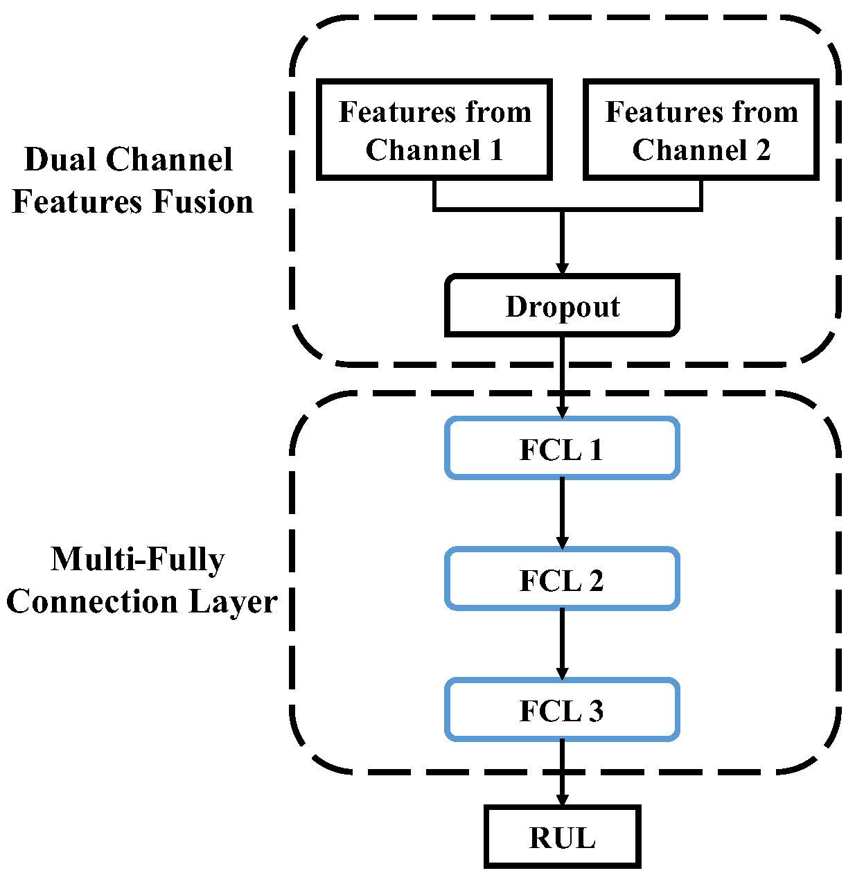
Based on the multi-layer full connection layer, a dual-channel feature fusion technique is implemented into the RUL prediction network. This improvement contributes to guaranteeing RUL prediction accuracy at the degradation stage.

(3)

The experimental results show that the RUL prediction method proposed in this study can extract more common degradation information from the various rolling bearing frequency bands. It shows the guaranteed reliability and universality of RUL prediction when compared with current mainstream approaches.

The following are the remaining sections of this study: Section 2 explains the proposed method’s theoretical foundation; Section 3 describes the improved method and its parameter optimization procedure; Section 4 is the experimental design and results analysis; Section 5 is the conclusion.

2. Methods

This study offers an innovative strategy for improving the feature extraction effect and prediction accuracy. Before describing the proposed approach, this section will briefly overview the theory of the related methods of the vision transformer and Swin transformer to understand the improved approach better.

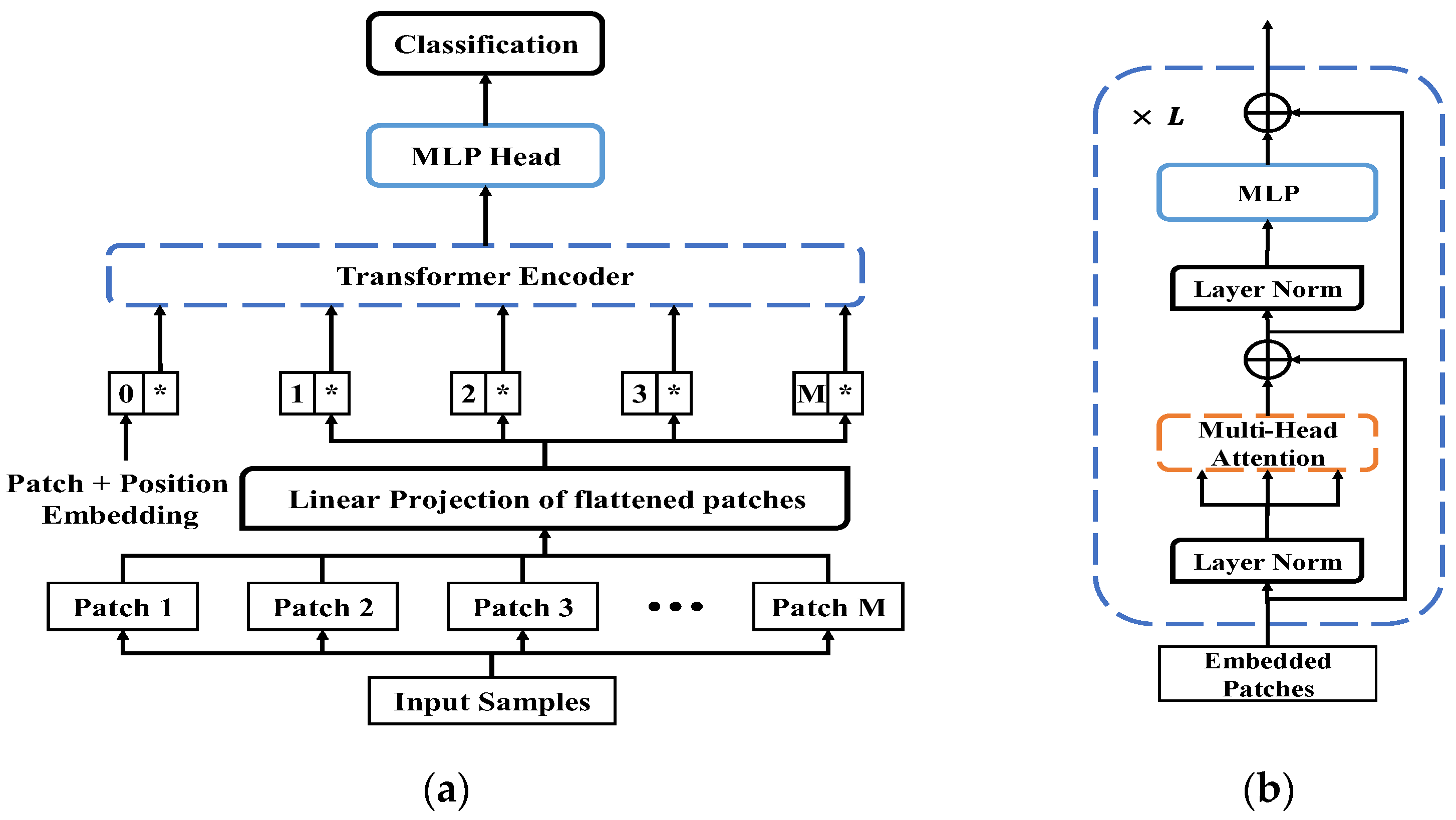
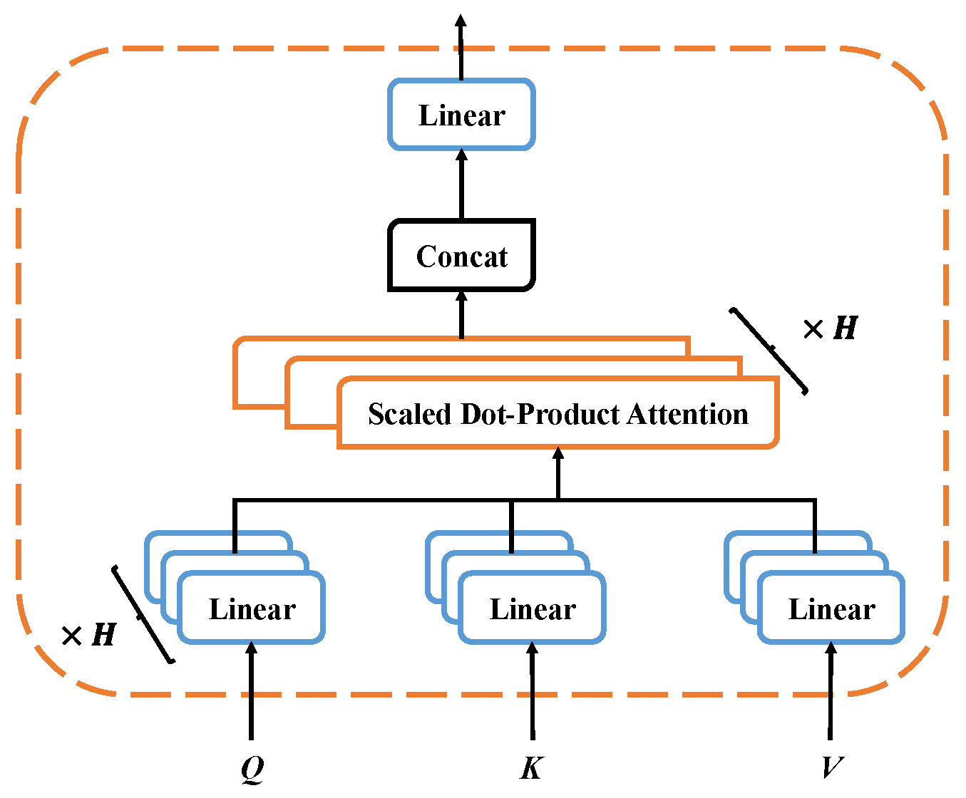
2.1. Vision Transformer

The transformer, which is one of the most traditional DL networks in natural language recognition, exclusively employs the attention mechanism (AM) to extract high-reliability depth features from temporally correlated input samples [39]. Dosovitskiy et al. [40] were inspired by this and proposed the Vision Transformer (ViT) network structure, as shown in Figure 1. Firstly, the high-dimensional input sample is turned into patches, which are flattened by linear projection to provide a series of samples with correlation. Based on the benefits of the transformer network, converted samples containing all patches are utilized as the input of networks to achieve depth feature extraction. This network builds the transformer encoder with multi-head self-attention (MSA), shown in Figure 2. MSA first carries out mapping projection on query matrix $Q$, key matrix $K,$ and value matrix $V$ through some different linear transformations. Finally, the converted results are spliced and concatenated to extract trustworthy and efficient depth features. Scaled dot-product is used in AM to address the issue that multi-linear transformation increases network complexity while decreasing processing speed.

$$MultiHead\left(Q,K,V\right)=Concat({Head}_1,{Head}_2,\dots ,{Head}_i)W^o$$

(1)

$${Head}_i\left(Q,K,V\right)=Attention(Q{W}_i^Q,K{W}_i^K,V{W}_i^V)$$

(2)

$$Attention(Q{W}_i^Q,K{W}_i^K),V{W}_i^V=softmax[\frac{Q{W}_i^Q{\left(K{W}_i^K\right)}^T}{\sqrt{d_k}}]V{W}_i^V$$

(3)

Moreover, sine and cosine functions of different frequencies are employed in ViT networks to add relative position information and solve the gradient disappearance problem in previous deep recursive models.

$$PE\left(pos,2i\right)=sin(\frac{pos}{{10000}^{2i/d_{model}}})$$

(4)

$$PE\left(pos,2i+1\right)=cos(\frac{pos}{{10000}^{2i/d_{model}}})$$

(5)

2.2. Swin Transformer

Because a single patch size is utilized in the feature extraction procedure of ViT, features containing essential information cannot be fully and accurately acquired. Furthermore, the ViT model’s complicated network structure increases model complexity, which has numerous disadvantages for engineering applications. Liu et al. [38] proposed a ViT derivative network of the Swin transformer given the above problems. The network structure is shown in Figure 3. The shift windows processing of each patch for Each transformer block input is applied on the classic ViT network to realize the adaptive sealing extraction of depth information in the input sample and further improve the identification effect.

Firstly, the input sample $H\times W$ is divided into patches $\frac{H}{C}\times \frac{W}{C}$, with the Swin transformer block extracting the depth features of the containing interdependence. $C$ is the number of patch groups divided. Two successive Swin transformer block is shown in Figure 3b. The network’s features are extracted using window multi-head self-attention (WMSA) and shift window multi-head self-attention (SWMSA). Assuming that the input Swin Transformer block feature is $Z^{l-1}$, WMSA output feature ${\mathrm{Z}}^l$ and multi-layer perceptron (MLP) module output feature $Z^l$ corresponds to block $l$ is shown as follows, respectively:

$${\widehat{Z}}^{l-1}=WMSA\left(LN\left(Z^{l-1}\right)\right)+Z^{l-1}$$

(6)

$$Z^l=MLP\left(LN\left({\widehat{Z}}^l\right)\right)+{\widehat{Z}}^l$$

(7)

The SWMSA output feature ${\widehat{Z}}^{l+1}$ and MLP module output feature $Z^{l+1}$ corresponds to block $l+1$ is shown as follows respectively:

$${\widehat{Z}}^{l+1}=SWMSA\left(LN\left(Z^l\right)\right)+Z^l$$

(8)

$$Z^{l+1}=MLP\left(LN\left({\widehat{Z}}^{l+1}\right)\right)+{\widehat{Z}}^{l+1}$$

(9)

$LN$ denotes the layer normalization operation, which normalizes all neuron nodes in each layer of a single sample. $MLP$ is to calculate the features extracted from input samples by multiple perceptrons, and the specific calculation equation is shown in (10). WMSA and SWMSA represent window MSA that have been set with rules and shifted window divisions, respectively.

$$MLP\left(X\right)=W_O\phi \left(W_{H}X+b_H\right)+b_O$$

(10)

where $W_O$ and $W_H$ are corresponding weights of different perceptions. $b_O$ and $b_H$ are the corresponding deviations of different perceptions. $\phi (·)$ is the multilayer perceptron activation function.

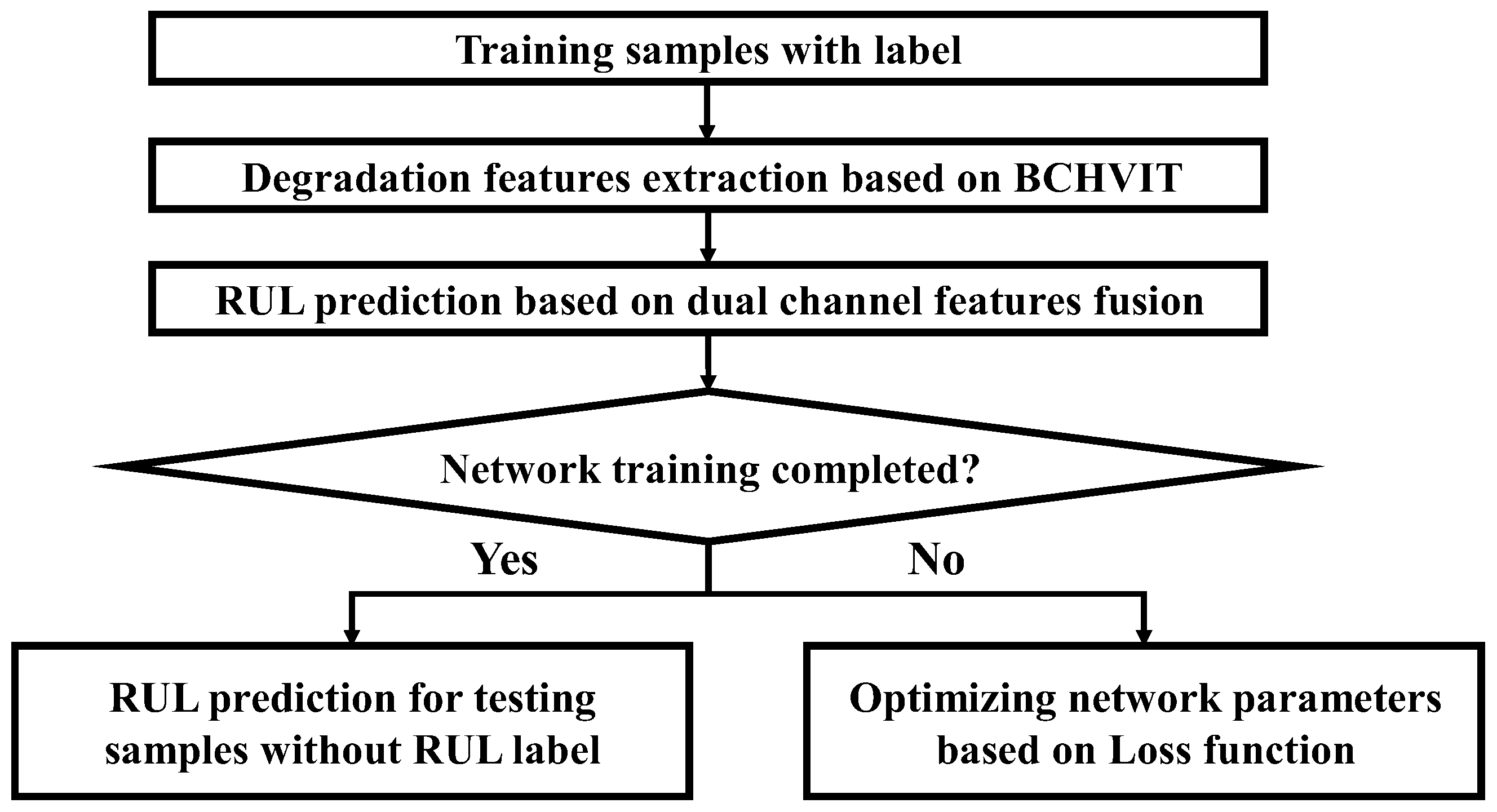
3. RUL Prediction Method Based on BCHViT

This study proposes an RUL prediction approach based on BCHViT to extract and employ highly correlated and diversified depth features in the degradation process for accuracy improvement. The whole RUL prediction network structure and process are shown in Figure 4. The proposed method’s main structure includes degradation feature extraction based on BCHViT and RUL prediction based on dual channel feature fusion, which is described in detail below.

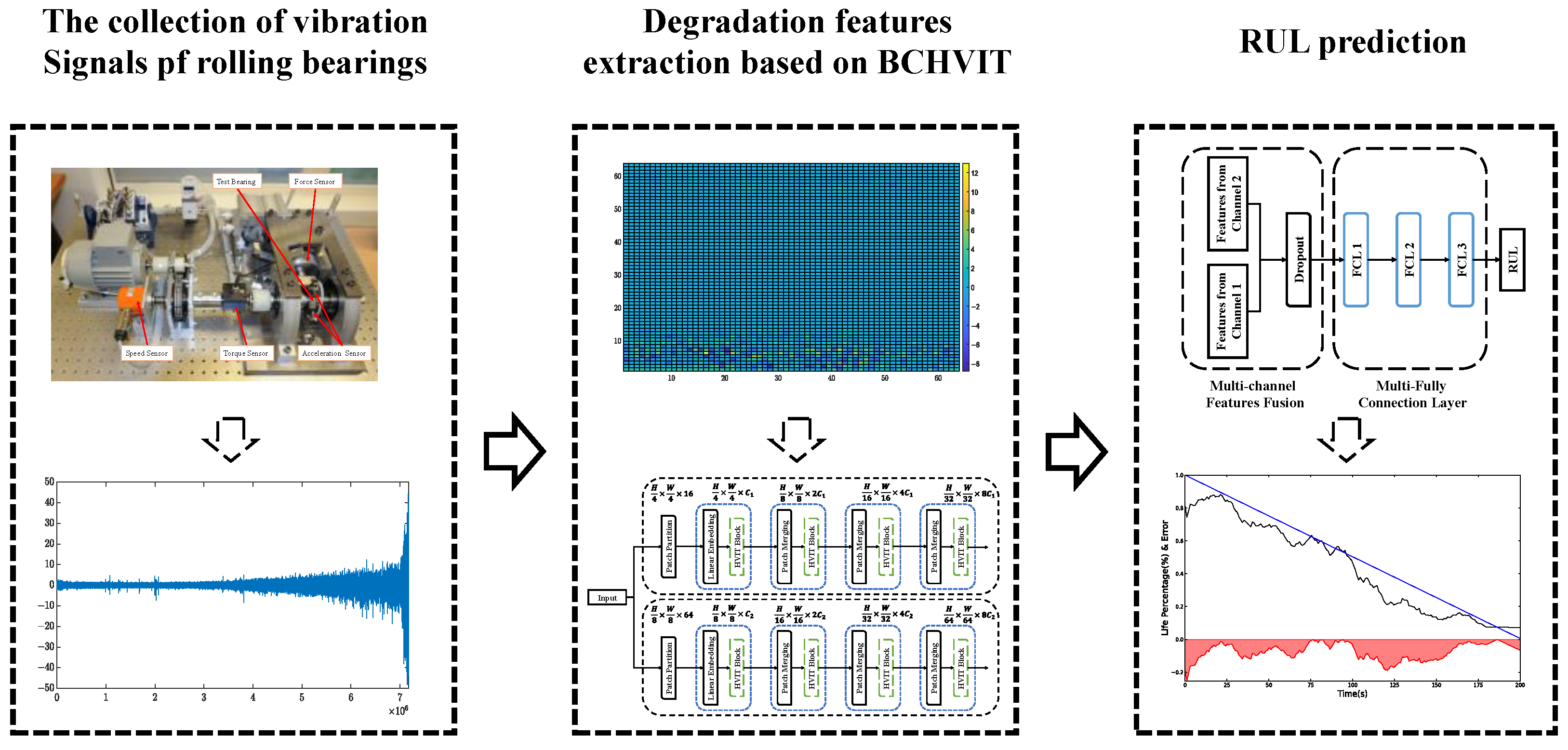
3.1. Degradation Feature Extraction Based on BCHViT

This study proposes a depth feature extraction method based on BCHViT inspired by the Swin transformer. The network structure is shown in Figure 5. As network input, wavelet packet coefficient samples of vibration signal decomposed by wavelet packet are employed. Wavelet packet coefficients $x_{j,m}\left(n\right)$, as an important part of wavelet packet decomposition [41], can effectively reflect the critical information of signals. It is the decomposition coefficient of signal $f\left(t\right)$ at scale $j$ for the wavelet packet function ${\mu }_{j,m}$. Its calculation formula is listed as follows.

$$\left\{\begin{array}{c}{x}_{j,2m}\left(n\right)=\sqrt{2}{\displaystyle \sum _{k\in Z}}h(k-2n)x_{j-1,m}\left(k\right)\\ x_{j,2m+1}\left(n\right)=\sqrt{2}{\displaystyle \sum _{k\in Z}}g(k-2n)x_{j-1,m}\left(k\right)\end{array}\right.$$

(11)

where $m$ denotes the frequency band. The higher the value of $m$; the higher the frequency band in which the coefficients are located; $n$ indicates the time domain location; $g(·)$ and $h(·)$ denote the high-pass filtering function and the low-barrel filtering function, respectively.

Although wavelet packet coefficients can efficiently reflect high- and low-frequency information in vibration signal samples, this property cannot be employed directly for RUL prediction. Swin transformer has excellent depth feature extraction capacity, but the influence of patch size restricts its ability to be improved further. As a result of the wavelet packet co-efficient features, SWMSA and WMSA in the Swin transformer block also have a negative impact.

BCHViT is offered in this work to overcome the difficulties described above. Given the impact of patch size on depth feature extraction, two patches of different sizes are selected to extract dual channel depth feature $Z^{channel1}$ and $Z^{channel2}$. The extraction process of the dual channel depth feature is shown in Figure 5a. Firstly, the input sample $H\times W$ is segmented into different patches to extract the depth features by using the HVIT block from two different channels. Meanwhile, the HVIT block proposed in this study removes SWMSA and WMSA from the typical Swin transformer block. Two successive HVIT block is shown in Figure 5b. The relationship between the input HVIT block feature is $Z^{l-1}$ and output feature $Z^{l+1}$ is shown as follows.

$$Z^l=MLP\left(LN\left(Z^{l-1}\right)\right)+Z^{l-1}$$

(12)

$$Z^{l+1}=MLP\left(LN\left(Z^l\right)\right)+Z^l$$

(13)

The degradation feature extraction proposed in this study can reduce the model complexity while extracting high-value information from the original vibration signal. This innovative method can improve the effect of RUL prediction.

3.2. RUL Prediction Based on Dual Channel Feature Fusion

The RUL prediction network based on dual channel feature fusion is employed to realize the regression mapping between extracted depth degradation features and RUL, as illustrated in Figure 6. The dual-channel feature fusion is used to combine the depth features $Z^{channel1}$ and $Z^{channel2}$ from two different channels. As a result, the dropout layer [42] is employed to improve the generalization of the RUL prediction and reduce the effect of overfitting.

$$Z^M=Dropout\left(Concat\right(Z^{channel1}{,Z}^{channel2}\left)\right)$$

(14)

Given that the present fully connected layer (FCL) has a positive predictive effect in RUL prediction [43], this network selects the fully connected network to build a regression mapping relationship between fusion features and RUL results. The following is the calculation formula for the first, second, and third layers:

$$Z^{h1}=ReLU(W_1{Z}^M+b_1)$$

(15)

$$Z^{h2}=ReLU(W_2{Z}^{h1}+b_2)$$

(16)

$$Z^{h3}=ReLU(W_3{Z}^{h2}+b_3)$$

(17)

where $Z^{h1}$,$Z^{h2}$,$Z^{h3}$ are the outputs of FCL 1, FCL 2, and FCL 3, respectively.$W_1$, $W_2$, and $W_3$ are the weight matrices of each FCL, respectively. $b_1$, $b_2$, and $b_3$ are the bias of each FCL, respectively. $Z^{h3}$ is the final prediction result of the RUL prediction network.

3.3. Model Optimization Objective and Training Process

The flow chart of networks proposed in this study is shown in Figure 7. As model training input, this network picks the wavelet packet coefficients of rolling bearings with labels. The Adam algorithm and optimization objective are used to optimize network parameters to significantly increase RUL’s prediction accuracy.

The model proposed in this study is based on supervised training. The specific algorithm flow is shown in Algorithm 1. It is assumed that the input sample is $X,$ and the minimum batch of the sample is $m$. The training data extraction from degenerate samples with labels is ${\{x_i,y_i\}}_{i=\mathrm{1,2},\dots ,N}^m$. The mapping functions of the degenerate feature extraction network and RUL prediction network are $f_F\left(x,{\theta }_F\right):R^k\to R^l$ and $f_R\left(x,{\theta }_R\right):R^l\to R^1$, respectively. ${\theta }_F$ and ${\theta }_R$ are training parameters of the degenerate feature extraction network and RUL prediction network.

The optimization goal of the RUL prediction technique in this work is $L_{RUL}$, which is the mean square error between prediction results and labels. The following is the particular calculating formula:

$$L_{RUL}=\frac{1}{n}\sum _{i=1}^n{(f_R\left(z_i^M\right)-y_i)}^2$$

(18)

$$z_i^M={Concat(z}_i^{channel1}{,z}_i^{channel2})$$

(19)

$$z_i^{channel1}{,z}_i^{channel2}=f_F\left(x_i\right)$$

(20)

Algorithm 1. Description of algorithm flow

Input: sample $X=\{x_1,x_2,\dots ,x_n\}$, minimum batch $m$ 1. Initialization of parameters of networks, including ${\theta }_F$ and ${\theta }_R$ 2. do: 3. For $i=\mathrm{1,2},...,N_{}:$ 4.  Take $m$ samples ${\left\{x_i\right\}}^m$ from $X$ 5.  Extract degradation features based on BCHViT networks  $z_i^{channel1}{,z}_i^{channel2}\leftarrow f_F\left(x_i\right)$ 6.  Dual channel deep feature fusion  $z_i^M\leftarrow {Concat(z}_i^{channel1}{,z}_i^{channel2}$) 7.  Take samples ${\{z_i^M,y_i\}}^m$           ${\theta }_F,{\theta }_R\leftarrow {\theta }_F,{\theta }_R-\frac{1}{n}{\displaystyle \sum _{i=1}^n}{\left(f_R\left(z_i^M\right)-y_i\right)}^2$ 8.  Until ${\theta }_F$ and ${\theta }_R$ sum converges

$n$ is the number of samples. $z_i^{channel1}$ and $z_i^{channel2}$ are the degradation feature of the output depth of two channels, respectively. $z_i^M$ is the result of dual-channel feature fusion after two-channel depth degradation feature fusion.

$$\underset{{\theta }_F,{\theta }_R}{\min }Loss=\underset{{\theta }_F,{\theta }_R}{\min }\left\{L_{RUL}\right\}$$

(21)

The network proposed in this network optimizes the parameters by minimizing the loss function through an “end-to-end” supervised training process.

4. Experimental Verification and Analysis

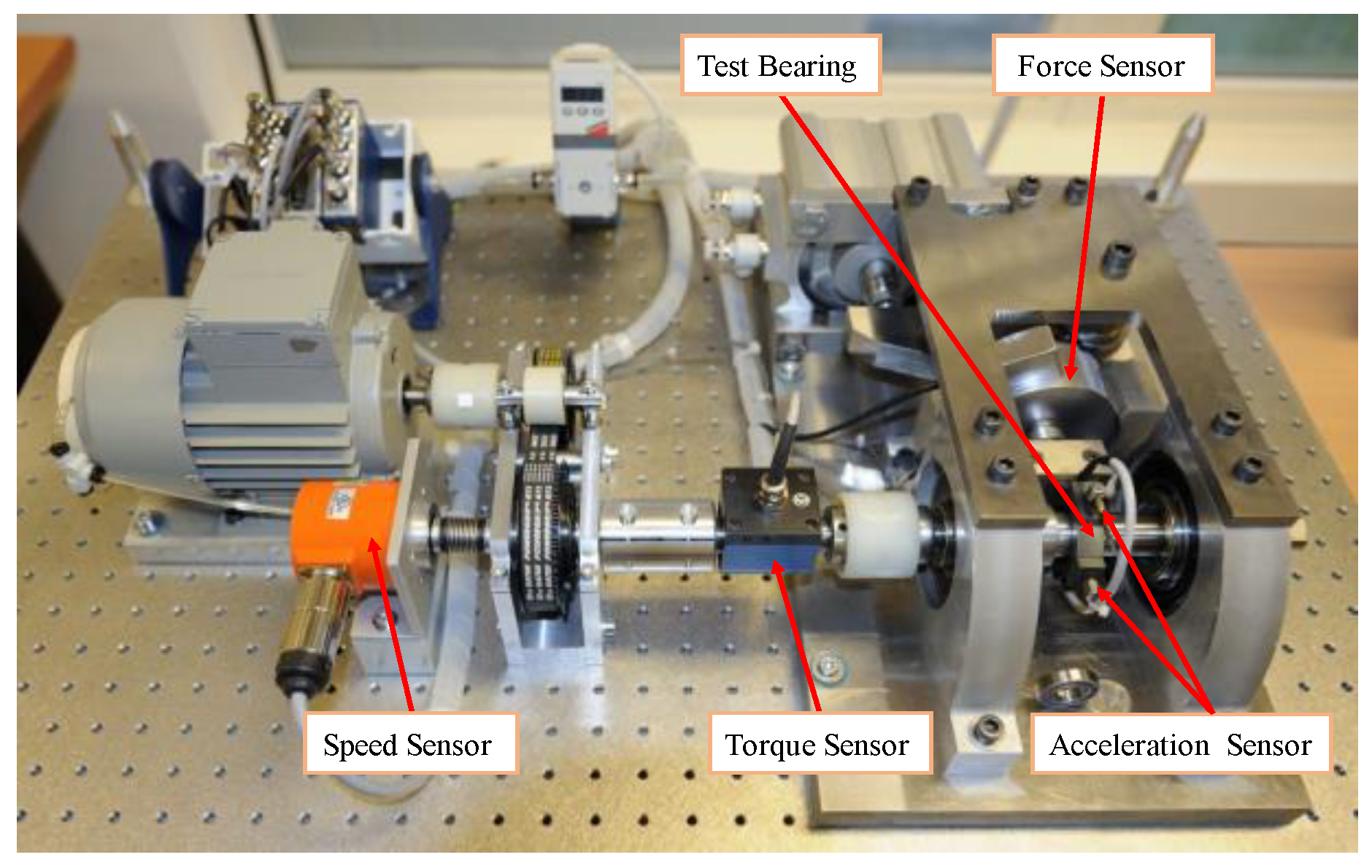
4.1. Experimental Data Introduction

The rolling bearing deterioration vibration signal dataset given by the IEEE PHM Data Challenge conducted in 2012 [44] was utilized to test the reliability of this study. Figure 8 shows the PRONOSTIA test Platform for collecting rolling bearing samples. The degrading vibration signals used in the verification were obtained from the acceleration measuring devices installed in this platform’s horizontal and vertical directions. The datasets contain vibration degradation information of 17 different rolling bearings. The sampling frequency of the data was 25.6 kHz. The samples were taken every 10 s with a 0.1 s collection interval, totaling 2560 data points.

Table 1. Description of working conditions of PHM challenge 2012 bearing dataset.

Name	Condition 1	Condition 2	Condition 3
Load (N)	4000	4200	5000
Motor Speed (rpm)	1800	1650	1500
Number of Bearings	7	7	3
Name of Bearings	1-1,1-2,1-3,1-4,1-5,1-6,1-7	2-1,2-2,2-3,2-4,2-5,2-6,2-7	3-1,3-2,3-3

shows how 17 sets of data samples are separated into three operating situations based on the difference in load and motor speed.

4.2. Experimental Data Pre-Processing

The pre-processing approach used in this study is wavelet packet decomposition. As the network’s input, the wavelet packet coefficients are employed. The DB13 wavelet is chosen as the wavelet basis to facilitate the classification of patches and hierarchical depth feature extraction for each collection of 2560 degenerate vibration samples. After wavelet packet decomposition, the original 2560 rolling bearing vibration signals are transformed into 64 × 64 two-dimensional wavelet packet coefficient samples. Samples before and after processing are shown in Figure 9. According to the method in [35], the rolling bearing degradation process generates degradation labels between [0, 1]. This degradation label is conducive to using the gradient descent algorithm to solve the DL network optimization process and improve the prediction accuracy of RUL.

4.3. The Experiment Designs

4.3.1. Experimental Arrangement and Evaluation Index

The proposed method in this study is constructed and trained using Pytorch on a Windows 10 and Python platforms. The training device has a CPU i5-9400, a GPU GTX 1650, and 8 GB RAM.

Test 1 evaluates the influence of differences in working conditions. As a result, only the training and test sets for samples of the same working condition are divided in this experimental arrangement. Throughout the experiment, a single bearing degradation sample was chosen as the test dataset and the others as the training set samples. Because the number of datasets differed across the working condition, seven verification experiments were put up under working conditions 1 and 2, respectively. In comparison, only three verification experiments were set up under working conditions 3. Because of the limited space available, only Bearings 1-2, 2-2, and 3-2 are used as examples to demonstrate the unique experimental arrangements shown in

Table 2. The specific experimental arrangement of 1-2,2-2, and 3-2 in Test 1.

Testing Bearing	Training Datasets	Testing Datasets
Bearing 1-2	1-1,1-3,1-4,1-5,1-6,1-7	1-2
Bearing 2-2	2-1,2-3,2-4,2-5,2-6,2-7	2-2
Bearing 3-2	3-1,3-3	3-2

under different working conditions.

This study used two sets of validation tests, called Test 1 and Test 2, to validate the reliability and generality of the proposed method. Test1 was utilized for experimental ablation and experimental comparison validation because of the maximum control of influencing factors. Test 2 validates the training model’s prediction accuracy using all historical samples. It is more suited for engineering application scenarios. Test 2 validates the training model’s prediction accuracy using all historical samples. While the suggested method’s engineering application value is highlighted in this validation experiment, Test 2 is only used in comparative analysis with other methods.

In practice, obtaining samples of the whole life cycle of rolling bearings is difficult. As a result, historical samples collected under different working conditions are utilized for training the model in real engineering in Test 2. A single bearing degradation sample was chosen as the test dataset and the other 16 samples as the training dataset. Due to the restricted space available in this article, only 7 sets of rolling bearing degradation samples were chosen separately as the test dataset. The specific experimental arrangements are shown in

Table 3. The specific experimental arrangement in Test 2.

Testing Bearing	Training Datasets	Testing Datasets
Bearing 1-1	1-2,1-3,1-4,1-5,1-6,1-7, 2-1,2-2,2-3,2-4,2-5,2-6, 2-7,3-1,3-2,3-3	1-1
Bearing 1-2	1-1,1-3,1-4,1-5,1-6,1-7, 2-1,2-2,2-3,2-4,2-5,2-6, 2-7,3-1,3-2,3-3	1-2
Bearing 1-3	1-1,1-2,1-4,1-5,1-6,1-7, 2-1,2-2,2-3,2-4,2-5,2-6, 2-7,3-1,3-2,3-3	1-3
Bearing 1-4	1-1,1-2,1-3,1-5,1-6,1-7, 2-1,2-2,2-3,2-4,2-5,2-6, 2-7,3-1,3-2,3-3	1-4
Bearing 1-5	1-1,1-2,1-3,1-4,1-6,1-7, 2-1,2-2,2-3,2-4,2-5,2-6, 2-7,3-1,3-2,3-3	1-5
Bearing 1-6	1-1,1-2,1-3,1-4,1-5,1-7, 2-1,2-2,2-3,2-4,2-5,2-6, 2-7,3-1,3-2,3-3	1-6
Bearing 1-7	1-1,1-2,1-3,1-4,1-5,1-6, 2-1,2-2,2-3,2-4,2-5,2-6, 2-7,3-1,3-2,3-3	1-7

.

Because of the enormous quantity of testing sample data collected during the rolling bearings’ life cycle, 200 groups of samples with degradation labels were extracted from the test rolling bearings datasets using the equal interval descending sampling approach. The average absolute error (MAE) is used to evaluate these networks’ prediction accuracy. The computation formula is as follows:

$$\mathrm{M}\mathrm{A}\mathrm{E}=\frac{1}{n}\sum _{i=1}^n\left|\widehat{y_i}-y_i\right|$$

(22)

$\widehat{y_i}$ is the RUL prediction result. $y_i$ is the degradation label of the rolling bearing. $n$ is the total number of rolling bearing samples.

4.3.2. Parameter Setting

Model parameter Settings respectively include network parameters for extracting degradation features (as shown in

Table 4. Parameters of feature extraction network.

Parameters		Channel 1	Channel 2
Patch size		4	8
The dimension of patch embedding		24
Window size		4
Depth of each HViT layer		(2,2,6,2)
Number of attentions heads in different layer		(3,6,12,24)
Dropout Rate	Attention	0.2
	Stochastic	0.1
MLP ratio		3

) and network parameters for RUL prediction (as shown in

Table 5. Parameters of RUL prediction network.

No.	Name of layers	Units	Channel	Activation Function
1	FCL 1	(384,192)	1	ReLU
2	FCL 2	(192,64)	1	Leaky ReLU
3	FCL 3	(64,1)	1	ReLU

). The degradation feature extraction network is constructed utilizing two different-sized patches.

Each channel has four HViT layers, and each layer has a different number of attention heads. The network employs two dropout rates, attention one and stochastic one, to minimize the negative effects of over-fitting. The RUL predictive network has three full connection layers and one dropout layer. Only the second FCL employs the Leaky ReLU function rather than traditional ReLU activation to reduce silent neurons’ presence of silent neurons suitably. The dropout parameter of the RUL prediction network is set at 0.5.

This network was trained 10,000 times in each experiment using supervised “end-to-end” training. The training batch size is 100. The network’s initial learning rate is 1 × 10⁻⁴. The learning rate decreases as the network gradient increases. The training duration was 200 times, and the attenuation rate was 0.95. The Adam optimizer is employed for network optimization, and the L2 regularization coefficient is 0.1. To eliminate noise interference, the prediction results are smoothed using weighted average smoothing. The size of the sliding window is 11.

4.4. Results and Analysis

4.4.1. Ablation Experiments

The ablation experiment was set up to evaluate the efficacy of the proposed method. Swin Transformer and HViT with a single channel were carried out to validate the impact of the strategy presented in the study. Firstly, bearings 1-3 and bearings 2-6 were chosen as test samples to verify the predicted performance through the rolling bearing degradation process. The prediction results are shown in Figure 10a,b, respectively. As compared to the Swin transformer method, the special HViT proposed in this work can increase prediction accuracy. However, the working conditions influence this improvement in prediction accuracy. This prediction accuracy boost does not reflect the near-failure stages where the impact of the failure is most severe for bearings 2-6. RUL predictions in engineering are not guaranteed to be reliable. By utilizing BCHVit instead of HViT, the model’s prediction accuracy is insufficient at the near-failure stage. The impact of inadequate prediction performance improvement will be effectively reduced at the near-failure stages. The reason is that a feature extraction network based on BCHViT can extract more effective and diversified depth features that reflect the degradation process. The results show that the BCHViT can assure the engineering reliability of RUL predictions.

Statistical analysis of the experimental data was also performed, considering the influence of working conditions on prediction accuracy. The MAE of different rolling bearings for each working condition is shown in Figure 11. Because of the differences in individual degradation processes, the proposed approach in this study is unable to have a lower MAE value in each tested sample. However, as shown in Figure 11, the method proposed in this work can guarantee that more than 50% of the bearings have superior prediction accuracy when the number of training samples is more than condition 3. The experimental findings demonstrate that the proposed approach extracts critical depth features more effectively in the degradation process of rolling bearings under the same working conditions. This is essential to enhancing the RUL prediction method’s engineering generality.

Meanwhile, the average MAE at each working condition is also calculated in

Table 6. Statistical results of ablation experiment under the different working conditions in Test 1.

Working Condition	Swin Transformer	HViT	BCVHiT
Condition 1	${0.1574}_{-0.0869}^{+0.1253}$	${0.1517}_{-0.0808}^{+0.1383}$	${\mathbf{0.1326}}_{\mathbf{-}\mathbf{0.0640}}^{\mathbf{+}\mathbf{0.0768}}$
Condition 2	${0.2147}_{-0.0971}^{+0.1197}$	${0.1967}_{-0.1148}^{+0.0643}$	${\mathbf{0.1754}}_{\mathbf{-}\mathbf{0.0316}}^{\mathbf{+}\mathbf{0.0482}}$
Condition 3	${\mathbf{0.2525}}_{\mathbf{-}\mathbf{0.1138}}^{\mathbf{+}\mathbf{0.1341}}$	${0.2681}_{-0.0684}^{+0.0448}$	${0.2592}_{-0.0610}^{+0.0526}$
Average	${0.2082}_{-0.0508}^{+0.0443}$	${0.2055}_{-0.0538}^{+0.0626}$	${\mathbf{0.1891}}_{\mathbf{-}\mathbf{0.0565}}^{\mathbf{+}\mathbf{0.0701}}$

. As demonstrated by the statistical data, the method proposed in this study can maintain higher prediction accuracy under most working conditions. Compared with the Swin transformer and HViT, the proposed method improves average accuracy by 12.73% and 5.24%, respectively. This demonstrates that the novel method is more adaptive to the actual engineering demand.

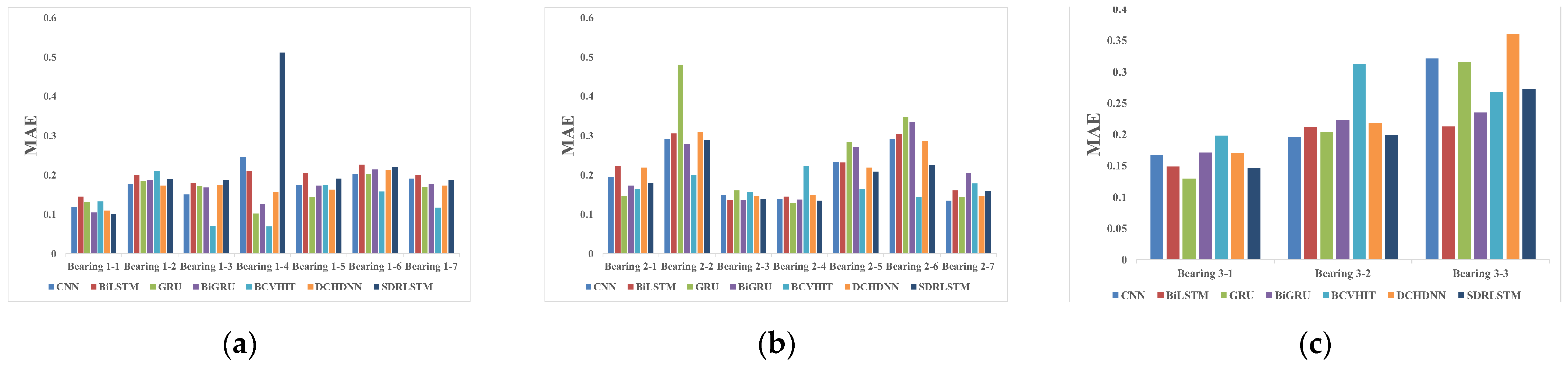
4.4.2. Comparative Analysis of Other Methods

Comparative tests were conducted in this study to verify the superiority of the proposed method further. CNN used in [45], Bi-LSTM used in [25], Bi-GRU used in [46], BiGRU used in [26], double-channel hybrid deep neural network based on CNN and BiLSTM (DCHDNN) used in [47], and stacked residuals deep LSTM (SRDLSTM) used in [48] were conducted for validation experiments. Because input samples include related wavelet packet coefficients of vibration signals that differ from the original model, all comparison methods except CNN employ a convolutional pooling network for degradation feature pre-extraction.

The experimental findings reveal that the suggested technique has a better prediction performance throughout the deterioration process, particularly at the near-failure stage. This suggests that the technique described in this work can better capture the exact moment of rolling bearing failure, making it more capable of meeting the predictive maintenance demands of mechanical equipment in actual engineering.

First, Bearing 1-3 and Bearing 2-6 are used to demonstrate the predictive performance of the RUL prediction method in the full degradation process. The RUL results are shown in Figure 12. The experimental results show that the proposed method has a higher prediction performance in the whole degradation process, particularly at the near-failure stage. This indicates that the approach proposed in this study can effectively reflect the exact moment of rolling bearing failure, making it more capable of satisfying the predictive maintenance requirements of mechanical equipment in actual engineering.

The RUL predicted accuracy of different rolling bearings under the three working conditions in Test 1 was then analyzed accordingly independently. The analysis results are shown in Figure 13 and

Table 7. Statistical results of the comparative method under the different working conditions in Test 1.

Method	Condition 1	Condition 2	Condition 3	Average
CNN	${0.1797}_{-0.0611}^{+0.0655}$	${0.2047}_{-0.0703}^{+0.0863}$	${0.2284}_{-0.0608}^{+0.0930}$	${0.2043}_{-0.0245}^{+0.0241}$
BiLSTM	${0.1948}_{-0.0505}^{+0.0308}$	${0.2148}_{-0.0796}^{+0.0902}$	${\mathbf{0.1909}}_{\mathbf{-}\mathbf{0.0419}}^{\mathbf{+}\mathbf{0.0215}}$	${0.2002}_{-0.0093}^{+0.0146}$
GRU	${0.1580}_{-0.0558}^{+0.0451}$	${0.2415}_{-0.1131}^{+0.2395}$	${0.2165}_{-0.0871}^{+0.0995}$	${0.2053}_{-0.0473}^{+0.0362}$
BiGRU	${0.1644}_{-0.0595}^{+0.0495}$	${0.2196}_{-0.0830}^{+0.1156}$	${0.2096}_{-0.0386}^{+0.0251}$	${0.1979}_{-0.0334}^{+0.0217}$
DCHDNN	${0.1883}_{-0.0749}^{+0.0845}$	${0.1754}_{-0.0789}^{+0.1185}$	${0.1969}_{-0.0541}^{+0.0520}$	${0.1959}_{-0.0076}^{+0.0065}$
SRDLSTM	${0.1657}_{-0.0564}^{+0.0476}$	${0.2107}_{-0.0646}^{+0.0979}$	${0.2500}_{-0.0795}^{+0.1110}$	${0.2088}_{-0.0431}^{+0.0412}$
BCHViT	${\mathbf{0.1326}}_{\mathbf{-}\mathbf{0.0640}}^{\mathbf{+}\mathbf{0.0768}}$	${\mathbf{0.1905}}_{\mathbf{-}\mathbf{0.0316}}^{\mathbf{+}\mathbf{0.0482}}$	${0.2592}_{-0.0610}^{+0.0526}$	${\mathbf{0.1891}}_{\mathbf{-}\mathbf{0.0565}}^{\mathbf{+}\mathbf{0.0701}}$

. Figure 13 indicates that the method proposed in this study can ensure better prediction accuracy for a greater amount of test rolling bearings. Table 7 demonstrates that the proposed approach can predict much better under more working conditions than other comparative approaches. The MAE is reduced by 7.42%, 5.53%, 7.90%, 4.44%, 9.43%, and 8.92%, respectively. The results demonstrate that the multi-channel method used in this study can extract features with more degraded correlation for RUL prediction than DCHDNN. After training with the same working sample, the experimental results in Test 1 indicate the superiority of the proposed method.

Finally, the experiments arranged in Test 2 were used to validate the proposed method’s excellence further. The experimental statistics are shown in

Table 8. Statistical results of different RUL prediction methods in Test 2.

Testing Bearing	CNN	Bi-LSTM	GRU	BIGRU	DCH-DNN	SRD-LSTM	BCVHIT
Bearing 1-1	0.1316	0.1670	0.0932	0.1267	0.1248	0.13405	0.1402
Bearing 1-2	0.1726	0.1829	0.1640	0.1815	0.1614	0.1873	0.0697
Bearing 1-3	0.1425	0.1637	0.1210	0.1281	0.1511	0.1633	0.1044
Bearing 1-4	0.2977	0.1314	0.0637	0.1389	0.3145	0.4106	0.0941
Bearing 1-5	0.1830	0.1976	0.1718	0.1731	0.1895	0.1855	0.0917
Bearing 1-6	0.2337	0.2078	0.2307	0.2193	0.2306	0.2243	0.2453
Bearing 1-7	0.1747	0.2093	0.1798	0.1798	0.1813	0.1929	0.1069
Average	0.1908	0.1800	0.1463	0.1639	0.1933	0.2140	0.1218

. The current study proposes methods for reducing the MAE to 36.20%, 32.34%, 16.78%, 25.72%, 37.02%, and 43.10%, respectively, when compared to the current mainstream prediction approaches. Because of the effect of different work conditions on the DL network is purposefully ignored in Test 2, the result shows that the depth features extracted by this proposed approach reflect the common information of the degradation process of different rolling bearings. This depth feature is more suitable for the current mechanical equipment to achieve RUL prediction based on DL.

5. Conclusions

An RUL prediction approach based on BCHViT is proposed further to improve the RUL prediction demands of rolling bearings and meet the essential maintenance needs of complicated mechanical equipment. Based on the Swin Transformer and rolling bearing degradation features, this approach innovatively optimizes the process of degradation feature extraction. To improve prediction accuracy, dual channel degrading feature fusion is included in the traditional RUL prediction network. The proposed method is effective, as evidenced by public datasets following conclusions are followed:

(1)

Compared to the Swin transformer model, the special HViT network structure proposed in this study can better use the DL network structure to extract depth features containing more significant degradation information. This feature meets the requirements of bearing RUL prediction in practical engineering by providing a higher prediction effect of RUL in the nearing failure stage.

(2)

Compared with current mainstream RUL prediction methods, the proposed method can extract depth features comprising degradation process common information from different rolling bearing degradation processes. This depth feature effectively ensures that the RUL prediction method is more general and accurate.

Although the method proposed in this study can effectively improve the RUL prediction accuracy of rolling bearings, the prediction accuracy will be decreased significantly when the rolling bearing degradation process is incomplete. In the future, the RUL prediction method based on the sample incompleteness condition will be carried out so that the RUL prediction model of rolling bearings based on DL can better meet practical engineering needs.

References

1. Ding, P.; Jia, M.; Zhao, X. Meta Deep Learning Based Rotating Machinery Health Prognostics toward Few-Shot Prognostics. Appl. Soft Comput. 2021, 104, 107211. [Google Scholar] [CrossRef]
2. Zhou, J.; Qin, Y.; Luo, J.; Wang, S.; Zhu, T. Dual-Thread Gated Recurrent Unit for Gear Remaining Useful Life Prediction. IEEE Trans. Industr. Inform. 2022, 1–11. [Google Scholar] [CrossRef]
3. Chen, M.; Shao, H.; Dou, H.; Li, W.; Liu, B. Data Augmentation and Intelligent Fault Diagnosis of Planetary Gearbox Using ILoFGAN Under Extremely Limited Samples. IEEE Trans. Reliab. 2022, 1–9. [Google Scholar] [CrossRef]
4. Hao, W.; Liu, F. Imbalanced Data Fault Diagnosis Based on an Evolutionary Online Sequential Extreme Learning Machine. Symmetry 2020, 12, 1204. [Google Scholar] [CrossRef]
5. Xiao, Y.; Shao, H.; Han, S.Y.; Huo, Z.; Wan, J. Novel Joint Transfer Network for Unsupervised Bearing Fault Diagnosis From Simulation Domain to Experimental Domain. IEEE/ASME Trans. Mechatron. 2022, 27, 5254–5263. [Google Scholar] [CrossRef]
6. Zou, Y.; Liu, Y.; Deng, J.; Jiang, Y.; Zhang, W. A Novel Transfer Learning Method for Bearing Fault Diagnosis under Different Working Conditions. Measurement 2021, 171, 108767. [Google Scholar] [CrossRef]
7. Hao, W.; Liu, F. Axle Temperature Monitoring and Neural Network Prediction Analysis for High-Speed Train under Operation. Symmetry 2020, 12, 1662. [Google Scholar] [CrossRef]
8. Li, N.; Lei, Y.; Guo, L.; Yan, T.; Lin, J. Remaining Useful Life Prediction Based on a General Expression of Stochastic Process Models. IEEE Trans. Ind. Electron. 2017, 64, 119–132. [Google Scholar] [CrossRef]
9. Ding, Y.; Ding, P.; Jia, M. A Novel Remaining Useful Life Prediction Method of Rolling Bearings Based on Deep Transfer Auto-Encoder. IEEE Trans. Instrum. Meas. 2021, 70, 2507812. [Google Scholar] [CrossRef]
10. Cheng, H.; Kong, X.; Chen, G.; Wang, Q.; Wang, R. Transferable Convolutional Neural Network Based Remaining Useful Life Prediction of Bearing under Multiple Failure Behaviors. Measurement 2021, 168, 108286. [Google Scholar] [CrossRef]
11. Wang, P.; Long, Z.; Wang, G. A Hybrid Prognostics Approach for Estimating Remaining Useful Life of Wind Turbine Bearings. IEEE Trans. Reliab. 2020, 6, 173–182. [Google Scholar] [CrossRef]
12. Lei, Y.; Li, N.; Guo, L.; Li, N.; Yan, T.; Lin, J. Machinery Health Prognostics: A Systematic Review from Data Acquisition to RUL Prediction. Mech. Syst. Signal Process. 2018, 104, 799–834. [Google Scholar] [CrossRef]
13. Cui, L.; Wang, X.; Wang, H.; Jiang, H. Remaining Useful Life Prediction of Rolling Element Bearings Based on Simulated Performance Degradation Dictionary. Mech. Mach. Theory 2020, 153, 103967. [Google Scholar] [CrossRef]
14. Li, Y.; Huang, X.; Ding, P.; Zhao, C. Wiener-Based Remaining Useful Life Prediction of Rolling Bearings Using Improved Kalman Filtering and Adaptive Modification. Measurement 2021, 182, 109706. [Google Scholar] [CrossRef]
15. Zeng, F.; Li, Y.; Jiang, Y.; Song, G. A Deep Attention Residual Neural Network-Based Remaining Useful Life Prediction of Machinery. Measurement 2021, 181, 109642. [Google Scholar] [CrossRef]
16. Yan, M.; Wang, X.; Wang, B.; Chang, M.; Muhammad, I. Bearing Remaining Useful Life Prediction Using Support Vector Machine and Hybrid Degradation Tracking Model. ISA Trans. 2020, 98, 471–482. [Google Scholar] [CrossRef]
17. Mishra, M.; Martinsson, J.; Goebel, K.; Rantatalo, M. Bearing Life Prediction with Informed Hyperprior Distribution: A Bayesian Hierarchical and Machine Learning Approach. IEEE Access 2021, 9, 157002–157011. [Google Scholar] [CrossRef]
18. Xiahou, T.; Zeng, Z.; Liu, Y. Remaining Useful Life Prediction by Fusing Expert Knowledge and Condition Monitoring Information. IEEE Trans. Industr. Inform. 2021, 17, 2653–2663. [Google Scholar] [CrossRef]
19. Zhang, K.; Tang, B.; Deng, L.; Tan, Q.; Yu, H. A Fault Diagnosis Method for Wind Turbines Gearbox Based on Adaptive Loss Weighted Meta-ResNet under Noisy Labels. Mech. Syst. Signal Process. 2021, 161, 107963. [Google Scholar] [CrossRef]
20. Li, Z.; Zhang, K.; Liu, Y.; Zou, Y.; Ding, G. A Novel Remaining Useful Life Transfer Prediction Method of Rolling Bearings Based on Working Conditions Common Benchmark. IEEE Trans. Instrum. Meas. 2022, 71, 3524909. [Google Scholar] [CrossRef]
21. Li, H.; Zhao, W.; Zhang, Y.; Zio, E. Remaining Useful Life Prediction Using Multi-Scale Deep Convolutional Neural Network. Appl. Soft Comput. J. 2020, 89, 87–96. [Google Scholar] [CrossRef]
22. Zou, Y.; Zhao, S.; Liu, Y.; Li, Z.; Song, X.; Ding, G. The Transfer Prediction Method of Bearing Remain Use Life Based on Dynamic Benchmark. IEEE Trans. Instrum. Meas. 2021, 70, 2516211. [Google Scholar] [CrossRef]
23. Han, T.; Pang, J.; Tan, A. Remaining Useful Life Prediction of Bearing Based on Stacked Autoencoder and Recurrent Neural Network. J. Manuf. Syst. 2021, 61, 576–591. [Google Scholar] [CrossRef]
24. Guo, L.; Li, N.; Jia, F.; Lei, Y.; Lin, J. A Recurrent Neural Network Based Health Indicator for Remaining Useful Life Prediction of Bearings. Neurocomputing 2017, 240, 98–109. [Google Scholar] [CrossRef]
25. Zou, Y.; Li, Z.; Liu, Y.; Zhao, S.; Liu, Y.; Ding, G. A Method for Predicting the Remaining Useful Life of Rolling Bearings under Different Working Conditions Based on Multi-Domain Adversarial Networks. Measurement 2021, 188, 110393. [Google Scholar] [CrossRef]
26. Fu, B.; Yuan, W.; Cui, X.; Yu, T.; Zhao, X.; Li, C. Correlation Analysis and Augmentation of Samples for a Bidirectional Gate Recurrent Unit Network for the Remaining Useful Life Prediction of Bearings. IEEE Sens. J. 2021, 21, 7989–8001. [Google Scholar] [CrossRef]
27. Wang, H.; Cheng, Y.; Song, K. Remaining Useful Life Estimation of Aircraft Engines Using a Joint Deep Learning Model Based on Tcnn and Transformer. Comput. Intell. Neurosci. 2021, 2021, 5185938. [Google Scholar] [CrossRef]
28. Zhao, S.; Zhang, C.; Wang, Y. Lithium-Ion Battery Capacity and Remaining Useful Life Prediction Using Board Learning System and Long Short-Term Memory Neural Network. J. Energy Storage 2022, 52, 104901. [Google Scholar] [CrossRef]
29. Ren, L.; Cui, J.; Sun, Y.; Cheng, X. Multi-Bearing Remaining Useful Life Collaborative Prediction: A Deep Learning Approach. J. Manuf. Syst. 2017, 43, 248–256. [Google Scholar] [CrossRef]
30. Zhang, K.; Tang, B.; Deng, L.; Liu, X. A Hybrid Attention Improved ResNet Based Fault Diagnosis Method of Wind Turbines Gearbox. Measurement 2021, 179, 109491. [Google Scholar] [CrossRef]
31. Zhang, C.; Zhao, S.; He, Y. An Integrated Method of the Future Capacity and RUL Prediction for Lithium-Ion Battery Pack. IEEE Trans. Veh. Technol. 2022, 71, 2601–2613. [Google Scholar] [CrossRef]
32. Su, X.; Liu, H.; Tao, L.; Lu, C.; Suo, M. An End-to-End Framework for Remaining Useful Life Prediction of Rolling Bearing Based on Feature Pre-Extraction Mechanism and Deep Adaptive Transformer Model. Comput. Ind. Eng. 2021, 161, 107531. [Google Scholar] [CrossRef]
33. Ding, Y.; Jia, M.; Cao, Y. Remaining Useful Life Estimation under Multiple Operating Conditions via Deep Subdomain Adaptation. IEEE Trans. Instrum. Meas. 2021, 70, 3516711. [Google Scholar] [CrossRef]
34. Cao, Y.; Ding, Y.; Jia, M.; Tian, R. A Novel Temporal Convolutional Network with Residual Self-Attention Mechanism for Remaining Useful Life Prediction of Rolling Bearings. Reliab. Eng. Syst. Saf. 2021, 215, 107813. [Google Scholar] [CrossRef]
35. Zeng, D.; Yang, J.; Zou, Y.; Zhang, J.; Song, X. Bearing Life Prediction Method Based on PMCCNN-LSTM. China Mech. Eng. 2020, 31, 2454–2462. [Google Scholar]
36. Zhang, C.; Zhao, S.; Yang, Z.; Chen, Y. A Reliable Data-Driven State-of-Health Estimation Model for Lithium-Ion Batteries in Electric Vehicles. Front. Energy Res. 2022, 10. [Google Scholar] [CrossRef]
37. Mao, W.; He, J.; Zuo, M.J. Predicting Remaining Useful Life of Rolling Bearings Based on Deep Feature Representation and Transfer Learning. IEEE Trans. Instrum. Meas. 2020, 69, 1594–1608. [Google Scholar] [CrossRef]
38. Liu, Z.; Lin, Y.; Cao, Y.; Hu, H.; Wei, Y.; Zhang, Z.; Lin, S.; Guo, B. Swin Transformer: Hierarchical Vision Transformer Using Shifted Windows. In Proceedings of the IEEE/CVF International Conference on Computer Vision, Montreal, QC, Canada, 10–17 October 2021. [Google Scholar]
39. Vaswani, A.; Shazeer, N.; Parmar, N.; Uszkoreit, J.; Jones, L.; Gomez, A.N.; Kaiser, Ł.; Polosukhin, I. Attention Is All You Need. Adv. Neural Inf. Process. Syst. 2017, 30, 5999–6009. [Google Scholar]
40. Dosovitskiy, A.; Beyer, L.; Kolesnikov, A.; Weissenborn, D.; Zhai, X.; Unterthiner, T.; Dehghani, M.; Minderer, M.; Heigold, G.; Gelly, S.; et al. An Image Is Worth 16x16 Words: Transformers for Image Recognition at Scale. arXiv 2020, arXiv:2010.11929. [Google Scholar]
41. Yen, G.G. Wavelet Packet Feature Extraction for Vibration Monitoring. IEEE Trans. Ind. Electron. 2000, 47, 650–667. [Google Scholar] [CrossRef] [Green Version]
42. Hinton, G.E.; Srivastava, N.; Krizhevsky, A.; Sutskever, I.; Salakhutdinov, R.R. Improving Neural Networks by Preventing Co-Adaptation of Feature Detectors. arXiv 2012, arXiv:1207.0580. [Google Scholar]
43. Zhu, J.; Chen, N.; Shen, C. A New Data-Driven Transferable Remaining Useful Life Prediction Approach for Bearing under Different Working Conditions. Mech. Syst. Signal Process. 2020, 139, 106602. [Google Scholar] [CrossRef]
44. Nectoux, P.; Gouriveau, R.; Medjaher, K.; Ramasso, E.; Chebel-morello, B.; Zerhouni, N.; Varnier, C.; Nectoux, P.; Gouriveau, R.; Medjaher, K.; et al. PRONOSTIA: An Experimental Platform for Bearings Accelerated Degradation Tests. To Cite This Version: HAL Id: Hal-00719503 PRONOSTIA: An Experimental Platform for Bearings Accelerated Degradation Tests. In Proceedings of the IEEE International Conference on Prognostics and Health Management, PHM’12, Denver, CO, USA, 20 June 2012; pp. 1–8. [Google Scholar]
45. Yao, D.; Li, B.; Liu, H.; Yang, J.; Jia, L. Remaining Useful Life Prediction of Roller Bearings Based on Improved 1D-CNN and Simple Recurrent Unit. Measurement 2021, 175, 109166. [Google Scholar] [CrossRef]
46. Xiao, L.; Liu, Z.; Zhang, Y.; Zheng, Y.; Cheng, C. Degradation Assessment of Bearings with Trend-Reconstruct-Based Features Selection and Gated Recurrent Unit Network. Measurement 2020, 165, 108064. [Google Scholar] [CrossRef]
47. Zhao, C.; Huang, X.; Li, Y.; Iqbal, M.Y. A Double-Channel Hybrid Deep Neural Network Based on CNN and BiLSTM for Remaining Useful Life Prediction. Sensors 2020, 20, 7109. [Google Scholar] [CrossRef]
48. Fu, S.; Zhang, Y.; Lin, L.; Zhao, M.; Zhong, S. sheng Deep Residual LSTM with Domain-Invariance for Remaining Useful Life Prediction across Domains. Reliab. Eng. Syst. Saf. 2021, 216, 108012. [Google Scholar] [CrossRef]
Figure 1. Vision transformer: (a) ViT’s structure; (b) Transformer encoder.
Processes 11 01153 g001
Figure 2. Multi-head attention of ViT.
Processes 11 01153 g002
Figure 3. Swin transformer network: (a) Network’s structure; (b) Swin transformer block.
Processes 11 01153 g003
Figure 4. The network structure of RUL prediction based on BCHViT.
Processes 11 01153 g004
Figure 5. Networks used for degradation feature extraction: (a) Network’s structure; (b) HVIT block.
Processes 11 01153 g005
Figure 6. RUL prediction networks based on dual channel feature fusion.
Processes 11 01153 g006
Figure 7. RUL prediction flow chart of this work.
Processes 11 01153 g007
Figure 8. PRONOSTIA test platform [44].
Processes 11 01153 g008
Figure 9. Visualization of raw signal and wavelet packet coefficient; (a) Raw signal at the beginning of the degradation process; (b) Wavelet packet coefficient at the beginning of the degradation process; (c) Raw signal at the end of the degradation process; (d) Wavelet packet coefficient at the end of the degradation process.
Processes 11 01153 g009
Figure 10. RUL prediction result of ablation experiment in Test 1: (a) Bearing 1-3; (b) Bearing 2-6.
Processes 11 01153 g010
Figure 11. The MAE of different rolling bearings for each working condition in the ablation experiment: (a) Condition 1; (b) Condition 2; (c) Condition 3.
Processes 11 01153 g011
Figure 12. RUL prediction result of different methods: (a) Bearing 1-3; (b) Bearing 2-6.
Processes 11 01153 g012
Figure 13. The MAE of different rolling bearings for each working condition in the comparative experiment: (a) Condition 1; (b) Condition 2; (c) Condition 3.
Processes 11 01153 g013