Stability Analysis: Two-Area Power System with Wind Power Integration

Abstract

This paper focuses on a comprehensive stability study of a two-area power system with wind power integration and synthetic inertia control in each area, considering the effects of varying the interconnection link. Normally, synthetic inertia proposals are analyzed in one-area systems, in which stability is tested without considering transmission system phenomena, such as coherency. As modern power systems are progressively becoming interconnected, the possibility of forming two or more non-coherent areas is likely, which poses a challenge to synthetic inertia control techniques that use system frequency as a main feedback signal. In this context, this work addresses a crucial gap in the existing literature and provides a valuable starting point for studying more complex interconnected power systems with wind power integration. Simulations were performed in Matlab-Simulink considering a data-driven frequency dynamics model of the Chilean Electric System, and a wind power model with synthetic inertia control $H_2$ norm minimization in each area. The results showed that it is possible to find local optimal feedback gains, preserving the stability of the global system under significant variations in the interconnection link. RoCoF and Nadir indicators are provided, highlighting the benefits of synthetic inertia control, particularly in low-inertia situations.

1. Introduction

Power systems have undergone a significant transformation due to the increased penetration of renewable energy sources (RES) interconnected through power electronics (such as solar and wind power), reducing system synchronous inertia. For example, a recent study has established that inertia in Europe has already begun to decrease, with a reduction of approximately 20% over the past two decades [1]. This situation represents a significant challenge for power system stability and operation due to the appearance of faster frequency dynamics, mentioned in [2,3]. As an example of the complexity of the new scenario, it is worth mentioning the event in the Southern California System on 16 August 2016, where the interruption of 1200 MW of solar power plants occurred. The event was caused by a low-inertia condition, which evolved into the activation of inverter protections based on instantaneous frequency measurement [4]. In 2019, a large-scale power outage of 1.5 h occurred in the UK, resulting in a 5% loss of total load [5]. In this scenario, the traditional hierarchical control scheme, comprising primary frequency control (PFC), secondary frequency control (SFC), and tertiary frequency control (TFC), seems to be insufficient to provide dynamic security if the power system continues on the same path toward increasing RES [6].

To preserve high-security levels, the role of the power electronics in future electric systems has been studied in the literature [7,8], and different control strategies have been proposed to deal with the new scenario [2,9]. In this sense, synthetic inertia (SI) control allows wind turbine kinetic energy transformation into fast electric power, emulating the inertial behavior of a synchronous generator [10,11]. SI, as an ancillary service, has been evaluated by various system operators, such as New Zealand [12], Canada [13], Great Britain, and Ireland [6,14].

A common aspect of existing SI techniques is that control schemes are designed and tested assuming that power systems can be described by one-machine equivalents, where the frequency is considered to be the same throughout the system. Modern power systems tend to interconnect, so the occurrence of large multi-area power systems with one or more weak links is likely to occur [15]. This makes one-area power system modeling inaccurate, given the increasing chance of inter-area oscillations and the transient lack of coherency that produces frequency to behave differently in different areas. As SI control is based on frequency measurements, its stability under multi-area scenarios is of interest.

On the other hand, frequency control strategies for multi-area power systems have been extensively studied, but previous research has mainly focused on load frequency control (LFC), automatic generation control (AGC), and PFC, overlooking SI frameworks. For example, the LFC problem has been studied in [16], where decentralized model predictive control (DMPC) is used. Additionally, in [17,18], the control problem is addressed by incorporating robust predictive control. A modern approach is presented in [19], where bald eagle sparrow PID control techniques are applied. The LFC and AGC combined problem is studied in [20], where integral (I), proportional-integral (PI), and proportional–integral–derivative (PID) control techniques are applied. The PFC problem is presented in [21], and the solution considers DMPC control.

In terms of SI control techniques, the published works have predominantly focused on one-area power systems or highly simplified test networks. In [22], the stability of a multi-wind turbine system is presented, but it does not consider the extrapolation of the results to multi-area power systems. In [23], an SI control strategy for variable-speed wind turbines (VSWT) in the Argentine–Uruguayan power system is described, but it is based on an on-off scheme applied to a one-area power system. Moreover, ref. [24] presents a comprehensive classification of SI control techniques in power systems with a high penetration of renewables, but the focus is on the control technique and does not include the power system model. In contrast, ref. [25] employs the kinetic energy reserve of the rotor from VSWT and the electrostatic energy stored in the supercapacitor units interfaced with its DC link to provide the inertial response and performs a modal analysis. It should be noted that the power system model utilized in this study was based on a simplified two-area test network, and the SI control technique was not described in detail. Additionally, only the frequency of the power system was considered as a feedback variable to perform the SI-VSWT control. This limitation is important to be noted when interpreting the results, as the behavior of more complex power systems can differ significantly.

Considering the state of the art described above, the following question arises: what is the impact on global stability when distinct regions, each containing wind power generation with optimal local SI control, are interconnected by transmission lines that can switch over time?

To answer this question, this paper focuses on the effect on global stability in a two-area power system with an interconnection link whose equivalent impedance can vary over time due to transmission switching and when each area is equipped with a decentralized synthetic inertia control. This work fills a literature gap and provides insight into the behavior of modern interconnected systems as they become interconnected over increasingly large geographical areas.

Therefore, the article’s structure is as follows: Section 2 consists of the problem formulation, which includes a concise model to obtain the frequency response of a two-area power system, a description of wind power plant dynamics, and an overview of the optimal area SI control employed in the simulations. The study case and the corresponding results are presented in Section 3 and Section 4, respectively. Finally, Section 5 offers a detailed discussion and analysis, highlighting the advantages and limitations, drawing conclusions and recommendations, and outlining future research directions.

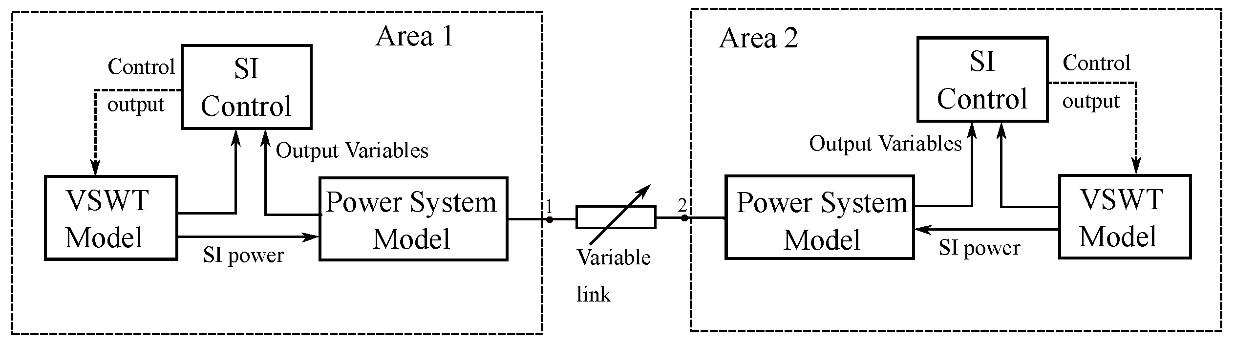
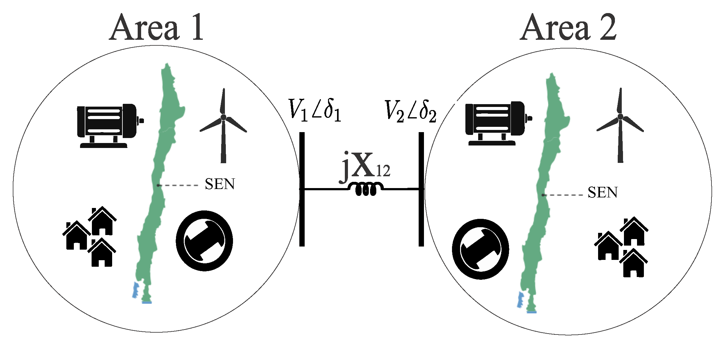
2. Problem Formulation

In this section, a general view of the problem to analyze in this work is presented. In this context, a two-area power system with wind power integration and SI control is shown in Figure 1. The input to the SI control is the power system and wind power variables, and the output is a torque reference signal to the electronic converter, which allows a fast power transfer from the VSWT to the power system to improve the frequency response when a power imbalance occurs. The link signifies the structural interconnection between both areas, which fluctuates based on the operational status of the transmission lines.

This study employs state feedback control to stabilize each area, with the objective of minimizing the RoCoF, through an $H_2$-norm optimization problem. Simulations are conducted to account for variations in the link and to obtain a root locus diagram of the poles of each area and the global system. By analyzing the poles of the system, insight can be gained into the stability and dynamic behavior of the interconnected power system, which can ultimately lead to improvements in its overall performance.

Next, the dynamic model is presented.

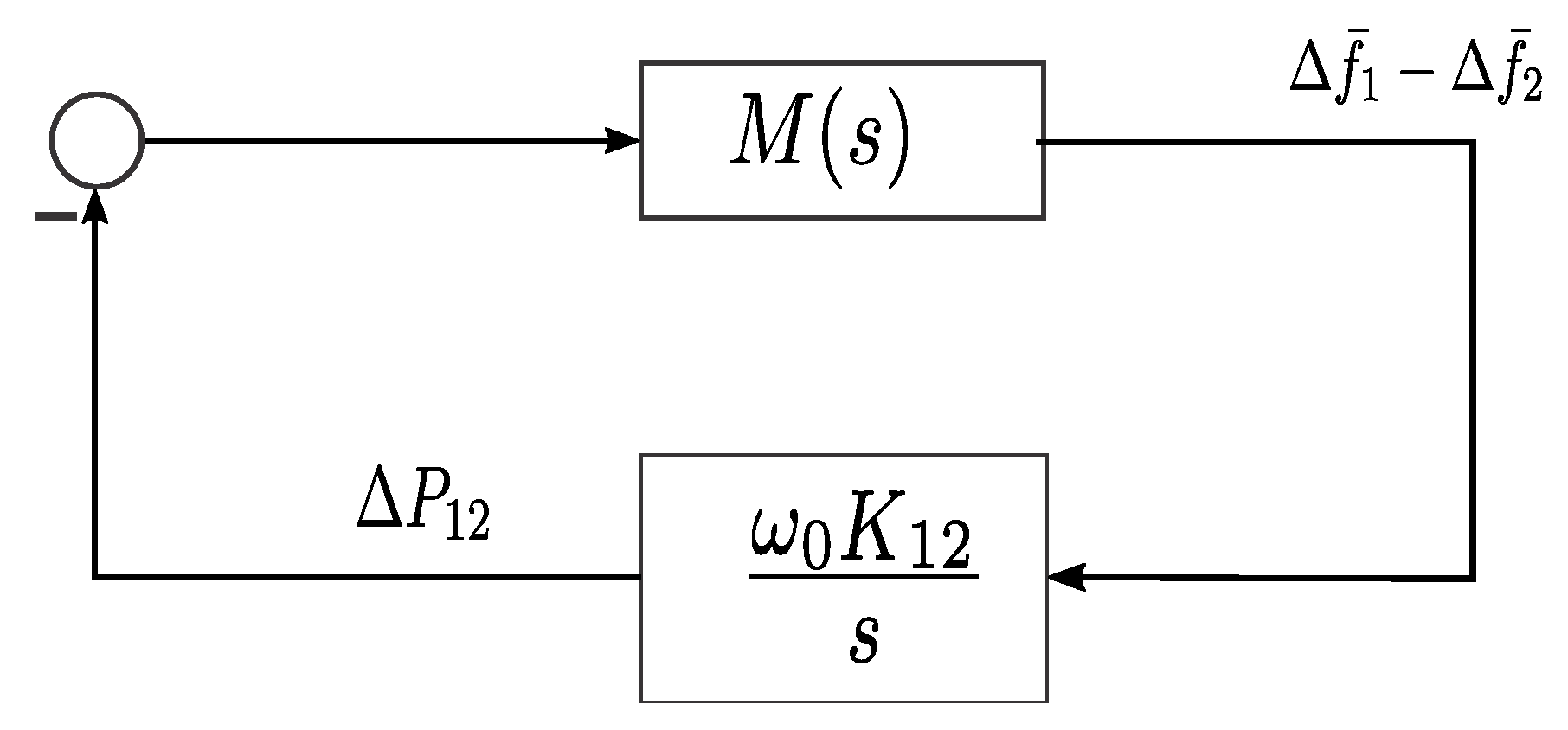
2.1. Power System Frequency Dynamic Model

This work considers a two-area power system model [26] that is a generalization of the simplified second-order governor-generator model used for one-area power system frequency studies, originally proposed in [27], and later, the parameter identification problem was included in [28]. The understanding of the way that important system parameters affect the frequency response is difficult to achieve in high order models, where the frequency performance is a complex function of many power system variables; therefore, the model allows a compromise between simplicity and accuracy.

The block diagram representation is shown in Figure 2, where, for each area i, $(i=1,2)$, the variable descriptions are as follows: $H_i=2K_{c_i}/f_0$ is an auxiliary variable, where $K_{c_i}$ represents the system’s kinetic energy in [MWs]; $f_0$ is the nominal system frequency in [Hz]; $K_{G_i}$ is the governor droop in [MW/Hz]; and ${\omega }_0$ is $2\pi f_0$.

The input of the system is the power imbalance $\mathrm{\Delta }{P}_{L_i}$ in [MW], and the output is the frequency $\mathrm{\Delta }{\overline{f}}_i$ in per-unit. Additionally, $\mathrm{\Delta }{P}_{m_i}$ represents the area governor power response in [MW].

The link representation $K_{12}$ denotes the synchronizing torque coefficient in [MW]. Its expression is derived through the linearization of the power exchange equations, as presented in (1), where $P_{12}$ is the power exchange between areas, and $V_1,V_2,{\delta }_{12}$ are the modules and the angular difference of the voltages of area-1 and area-2, in degrees and [kV], respectively. $X_{12}$ is the link equivalent reactance in [$\mathrm{\Omega }$].

$$P_{12}=\frac{V_1{V}_2}{X_{12}}sin{\delta }_{12}$$

(1)

The transfer function $G_i\left(s\right)$ is shown in (2). It is associated with the overall governor response [28], where $T_{a_i}$ and $T_{c_i}$ are in [s].

$$G_i\left(s\right)=\frac{(1+T_{c_i}s)}{(1+T_{a_i}s)},$$

(2)

Wind power can be added to the model by considering an incremental power contribution in each area, namely $\mathrm{\Delta }{P}_{w_1}$ and $\mathrm{\Delta }{P}_{w_2}$. In that case, the state-space equations that describe the system are:

$$\begin{array}{c}\hfill \begin{array}{cc}\hfill {\dot{x}}_{s_1}=& A_{s_1}{x}_{s_1}+A_{s_{13}}\mathrm{\Delta }{P}_{12}+B_{s_{w1}}\mathrm{\Delta }{P}_{L1}+B_{s_1}\mathrm{\Delta }{P}_{w1},\hfill \\ \hfill {\dot{x}}_{s_2}=& A_{s_2}{x}_{s_2}+A_{s_{23}}\mathrm{\Delta }{P}_{12}+B_{s_{w2}}\mathrm{\Delta }{P}_{L2}+B_{s_2}\mathrm{\Delta }{P}_{w2},\hfill \\ \hfill \mathrm{\Delta }{\dot{P}}_{12}=& K_{s_{12}}{x}_{s_1}-K_{s_{12}}{x}_{s_2},\hfill \end{array}\end{array}$$

(3)

where:

$$A_{s_1}=\left[\begin{array}{cc}0& -{\displaystyle \frac{1}{H_1}}\\ {\displaystyle \frac{K_{G_1}}{T_{a_1}}}& -{\displaystyle \frac{1}{T_{a_1}}}\left(1+{\displaystyle \frac{K_{G_1}{T}_{c_1}}{H_1}}\right)\end{array}\right],$$

(4)

$$A_{s_2}=\left[\begin{array}{cc}0& -{\displaystyle \frac{1}{H_2}}\\ {\displaystyle \frac{K_{G_2}}{T_{a_2}}}& -{\displaystyle \frac{1}{T_{a_2}}}\left(1+{\displaystyle \frac{K_{G_2}{T}_{c_2}}{H_2}}\right)\end{array}\right],$$

(5)

$$\begin{array}{cccc}\hfill A_{s_{13}}& =\left[\begin{array}{c}-{\displaystyle \frac{1}{H_1}}\\ {\displaystyle \frac{-K_{G_1}{T}_{c_1}}{H_1{T}_{a_1}}}\end{array}\right], \hfill & \hfill A_{s_{23}}& =\left[\begin{array}{c}{\displaystyle \frac{1}{H_2}}\\ {\displaystyle \frac{K_{G_2}{T}_{c_2}}{H_2{T}_{a_2}}}\end{array}\right],\hfill \end{array}$$

(6)

$$\begin{array}{cccc}\hfill B_{s_{w1}}& =\left[\begin{array}{c}-{\displaystyle \frac{1}{H_1}}\\ {\displaystyle \frac{-K_{G_1}{T}_{c_1}}{H_1{T}_{a_1}}}\end{array}\right], \hfill & \hfill B_{s_{w2}}& =\left[\begin{array}{c}-{\displaystyle \frac{1}{H_2}}\\ {\displaystyle \frac{-K_{G_2}{T}_{c_2}}{H_2{T}_{a_2}}}\end{array}\right],\hfill \end{array}$$

(7)

$$\begin{array}{cccc}\hfill x_{s_1}& =\left[\begin{array}{c}\mathrm{\Delta }{f}_1\\ \mathrm{\Delta }{P}_{m_1}\end{array}\right], \hfill & \hfill x_{s_2}& =\left[\begin{array}{c}\mathrm{\Delta }{f}_2\\ \mathrm{\Delta }{P}_{m_2}\end{array}\right],\hfill \end{array}$$

(8)

$$K_{s_{12}}=\left[\begin{array}{cc}{K}_{12}& 0\end{array}\right],$$

(9)

$$B_{s_1}=-B_{s_{w1}},B_{s_2}=-B_{s_{w2}},$$

(10)

Note that wind power injection is represented as a new input, with the opposite sign to $\mathrm{\Delta }{P}_{L_i}$.

Finally, the state-space equation of the overall system is:

$$\begin{array}{c}\hfill \begin{array}{cc}\hfill {\dot{x}}_s& =A_p{x}_s+B_{w}w+B_{u}u\hfill \\ \hfill y& =C{x}_s,\hfill \end{array}\end{array}$$

(11)

where:

$$A_p=\left[\begin{array}{ccc}{A}_{s_1}& 0& A_{s_{13}}\\ 0& A_{s_2}& A_{s_{23}}\\ K_{s_{12}}& -K_{s_{12}}& 0\end{array}\right],$$

(12)

$$\begin{array}{cccc}\hfill B_w& =\left[\begin{array}{cc}{B}_{s_{w1}}& 0\\ 0& B_{s_{w2}}\\ 0& 0\end{array}\right], \hfill & \hfill B_u& =-B_w,\hfill \end{array}$$

(13)

$$\begin{array}{cccc}\hfill w& =\left[\begin{array}{c}\mathrm{\Delta }{P}_{L_1}\\ \mathrm{\Delta }{P}_{L_2}\end{array}\right], \hfill & \hfill u& =\left[\begin{array}{c}\mathrm{\Delta }{P}_{w_1}\\ \mathrm{\Delta }{P}_{w_2}\end{array}\right],\hfill \end{array}$$

(14)

$$x_s={\left[\begin{array}{ccc}{x}_{s_1}& x_{s_2}& \mathrm{\Delta }{P}_{12}\end{array}\right]}^T.$$

(15)

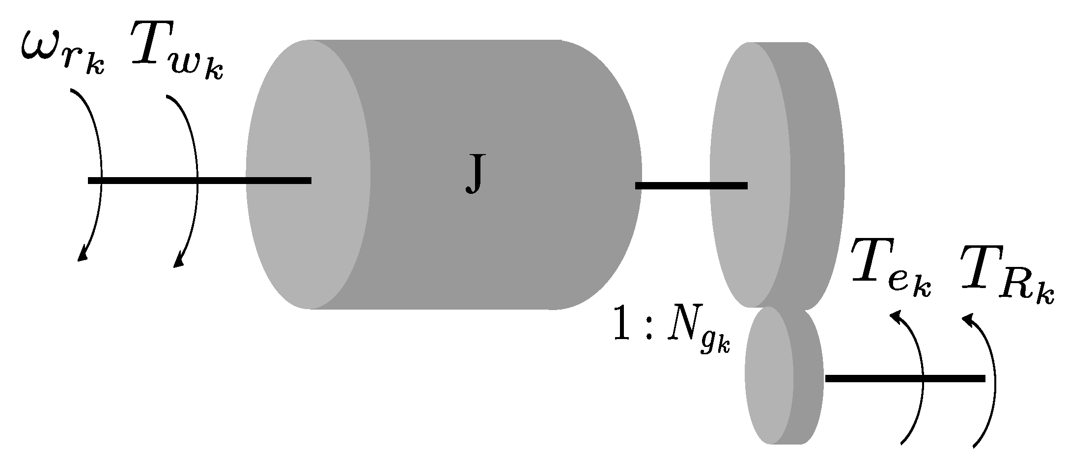
2.2. Wind Power Plant and SI Control

The one-mass VSWT model [22,29] is adjusted to incorporate SI control, as shown in Figure 3, with $k=1,2$.

The dynamic equations that describe the model are presented in (16).

$$\begin{array}{cc}\hfill {\dot{\omega }}_r& =\frac{1}{J}\left(T_w-N_g\left(T_e+T_R\right)\right),\hfill \\ \hfill T_w& =\frac{0.5\rho A{v}_w^3{C}_p}{{\omega }_r},\hfill \\ \hfill \mathrm{\Delta }{\dot{T}}_e& =N_g{K}_P\mathrm{\Delta }{\dot{\omega }}_r+N_g{K}_i\mathrm{\Delta }{\omega }_r,\hfill \\ \hfill C_p& =0.645\left(0.00912\lambda +\frac{-5-0.4\left(2.5+\beta \right)+116{\lambda }_i}{e^{21{\lambda }_i}}\right),\hfill \\ \hfill \lambda & =\frac{{\omega }_r·R_m}{v_w},\hfill \\ \hfill {\lambda }_i& =\frac{1}{\lambda +0.08(2.5+\beta )}-\frac{0.035}{1+{(2.5+\beta )}^3},\hfill \end{array}$$

(16)

where:

• ${\omega }_r$           VSWT angular speed (rad/s),
• J               VSWT combined moment of inertia (MNm$·{\mathrm{s}}^2$),
• $T_w$           VSWT mechanical torque (MNm),
• $T_e$             torque reference from MPPT control (MNm),
• $T_R$            torque reference from the SI control (MNm),
• $N_g$           gearbox speed ratio (-),
• $k_p,k_i$        proportional and integral gains of MPPT control,
• $v_w$            wind speed (m/s),
• $\rho$              air density (kg/${\mathrm{m}}^3$),
• $R_m$           rotor-swept radius (m)
• A             VSWT rotor-swept area (${\mathrm{m}}^2$),
• $C_p$           VSWT power coefficient,
• $\lambda$             VSWT tip speed ratio,
• $\beta$             VSWT pitch angle (${}^{\circ }$),

The numerical values of these parameters can be found in Appendix A. For control purposes, Equation (16) is linearized for area i as follows:

$$\begin{array}{cc}\hfill {\dot{\overline{x}}}_i& ={\overline{A}}_i{\overline{x}}_i+{\overline{B}}_i\mathrm{\Delta }{T}_{R_i},\hfill \\ \hfill \mathrm{\Delta }{P}_{w_i}& ={\overline{C}}_i{\overline{x}}_i+{\overline{D}}_i\mathrm{\Delta }{T}_{R_i},\hfill \end{array}$$

(17)

and the associated state space vector is:

$${\overline{x}}_i={\left[\mathrm{\Delta }{\omega }_{r_i}\mathrm{\Delta }{T}_{e_i}\right]}^T,$$

(18)

where: $\mathrm{\Delta }{\omega }_{r_i}$ ∈ $\mathbb{R}$ and $\mathrm{\Delta }{T}_{e_i}\in \mathbb{R}$ are the speed deviation and the electrical torque deviation from the operating point of the VSWT, respectively.

The matrices ${\overline{A}}_i\in {\mathbb{R}}^{2\times 2}$, ${\overline{B}}_i\in {\mathbb{R}}^{2\times 1}$, ${\overline{C}}_i\in {\mathbb{R}}^{1\times 2}$, and ${\overline{D}}_i\in {\mathbb{R}}^{1\times 1}$ are obtained from the linearization process.

A decentralized SI control is considered in each area, according to Figure 4, where the dynamic interactions between one turbine and its corresponding power system are shown. The control gains $K_1$ and $K_2$ are calculated to achieve stability in each area independently, as described below.

2.3. Optimal Area SI Controller

Consider a constant linear multivariable system equivalent to (11) that, for simplicity, is rearranged in (19):

$$\dot{x}=Ax+Bu,x\left(0\right)=x_0,$$

(19)

To design a linear quadratic optimal regulator (LQR) that determines an optimal feedback controller $u=Kx$, it is necessary to minimize the following quadratic performance index:

$$J(x,u)={\int }_0^{\infty }\left(x^{T}Qx+u^{T}Ru\right)dx,$$

(20)

where,

$$Q=Q^T\ge 0,R=R^T>0.$$

(21)

The result is based on the assumptions that:

$$\begin{array}{cc}\hfill (A,B)& \mathrm{is}\mathrm{stabilizable},\hfill \\ \hfill (A,L)& \mathrm{is}\mathrm{observable},\hfill \end{array}$$

(22)

with $L=Q^{1/2}$. If that conditions hold, then the Riccati equation:

$$A^{T}P+PA-PB{R}^{-1}{B}^{T}P+Q=0$$

(23)

has a unique symmetric positive definite solution P, and the optimal solution of the LQR problem is:

$$u\left(t\right)=-R^{-1}{B}^{T}Px\left(t\right)$$

(24)

and the minimum value of the performance index is

$$\gamma =\underset{u}{min}J(x,u)=x_0^{T}P{x}_0.$$

(25)

To ensure that the optimization process results in minimizing the RoCoF of the area, it is advisable to associate it with the performance of $H_2$. The following relation holds:

$$J(x,u)=\parallel G_{y\overline{\omega }}{\left(s\right)\parallel }_2^2$$

(26)

where $G_{y\overline{\omega }}\left(s\right)$ is the transfer function of the auxiliary system,

$$\begin{array}{cc}\hfill \dot{x}& =Ax+Bu+x_0\overline{\omega },\hfill \\ \hfill y& =Cx+Du,\hfill \end{array}$$

(27)

and $\overline{\omega }$ is the impulse function.

Under the assumptions (22) of the LQR problem, the $H_2$ equivalent formulation states that the same feedback gain K exists, such that $J(x,u)<\gamma$ if, and only if, there exists $X\in {\mathbb{R}}^n,Y\in {\mathbb{R}}^r$, and $W\in {\mathbb{R}}^{r\times n}$ satisfying the LMI [30], shown in (28):

$$\begin{array}{cc}\hfill \left({A_s}_i{X}_i+{B_s}_i{W}_i\right)+{\left({A_s}_i{X}_i+{B_s}_i{W}_i\right)}^T+{B_w}_i{B_w}_i^T& <0\hfill \\ \hfill trace\left(Q_i^{1/2}{X}_i{\left(Q_i^{1/2}\right)}^T\right)+trace\left(Y_i\right)& <{\gamma }_i\hfill \\ \hfill \left[\begin{array}{cc}-Y_i& R_i^{1/2}{W}_i\\ {\left(R_i^{1/2}{W}_i\right)}^T& -X_i\end{array}\right]& <0,\hfill \end{array}$$

(28)

and the feedback gain in each area is calculated as:

$$K_i=W_i{X}_i^{-1}.$$

(29)

and, for each control area ($i=1,2$), a state feedback control of the form of:

$$u_i=K_i{x}_i,$$

(30)

exists. Integrating wind dynamics (17) and control law (30) in (11), and according to the diagram shown in Figure 4, the close-loop state equation of the global system is obtained, as presented in (31):

$$\begin{array}{c}\hfill \begin{array}{cc}\hfill \dot{x}& =A_{cl}x+B_{w}w\hfill \\ \hfill y& =Cx,\hfill \end{array}\end{array}$$

(31)

where the new state space vector is:

$$x={\left[\begin{array}{ccccc}{x}_{s_1}& {\overline{x}}_1& x_{s_2}& {\overline{x}}_2& \mathrm{\Delta }{P}_{12}\end{array}\right]}^T,$$

(32)

and the close loop state space matrix is:

$$A_{cl}=\left[\begin{array}{ccccc}{A}_{{cl}_1}& -B_{{sw}_1}{\overline{C}}_{{cl}_1}& 0& 0& A_{s_{13}}\\ {\overline{B}}_{{}_1}{K}_{a_1}& {\overline{A}}_{{cl}_1}& 0& 0& 0\\ 0& 0& A_{{cl}_2}& -B_{{sw}_2}{\overline{C}}_{{cl}_2}& A_{s_{23}}\\ 0& 0& {\overline{B}}_{{}_2}{K}_{a_2}& {\overline{A}}_{{cl}_2}& 0\\ K_{s_{12}}& 0& -K_{s_{12}}& 0& 0\end{array}\right],$$

(33)

where:

$$\begin{array}{c}\hfill \begin{array}{cc}\hfill A_{{cl}_i}& =A_{s_i}-B_{{sw}_i}{\overline{D}}_{{}_i}{K}_{a_i}\hfill \\ \hfill {\overline{A}}_{{cl}_i}& ={\overline{A}}_{{}_i}+{\overline{B}}_{{}_i}{K}_{b_i}\hfill \\ \hfill {\overline{C}}_{{cl}_i}& ={\overline{C}}_{{}_i}+{\overline{D}}_{{}_i}{K}_{b_i}.\hfill \end{array}\end{array}$$

(34)

The SI torque is related to the power system and wind power variables as follows:

$$\begin{array}{cc}\hfill \mathrm{\Delta }{T}_{R_i}& =K_{a_i}{x}_{s_i}+K_{b_i}{\overline{x}}_i,\hfill \end{array}$$

(35)

$$\begin{array}{cc}\hfill K_i& =\left[\begin{array}{cc}{K}_{a_i}& K_{b_i}\end{array}\right].\hfill \end{array}$$

(36)

The significance of what was explained is that an LQR problem can be solved using an $H_2$ problem of an auxiliary system in which the impulse function is the input. Since the state-space matrices are time-invariant and the impulse response is the derivative of the step response, the output y of (27) includes $\frac{df}{dt}$ or RoCoF, which can be minimized according to (26).

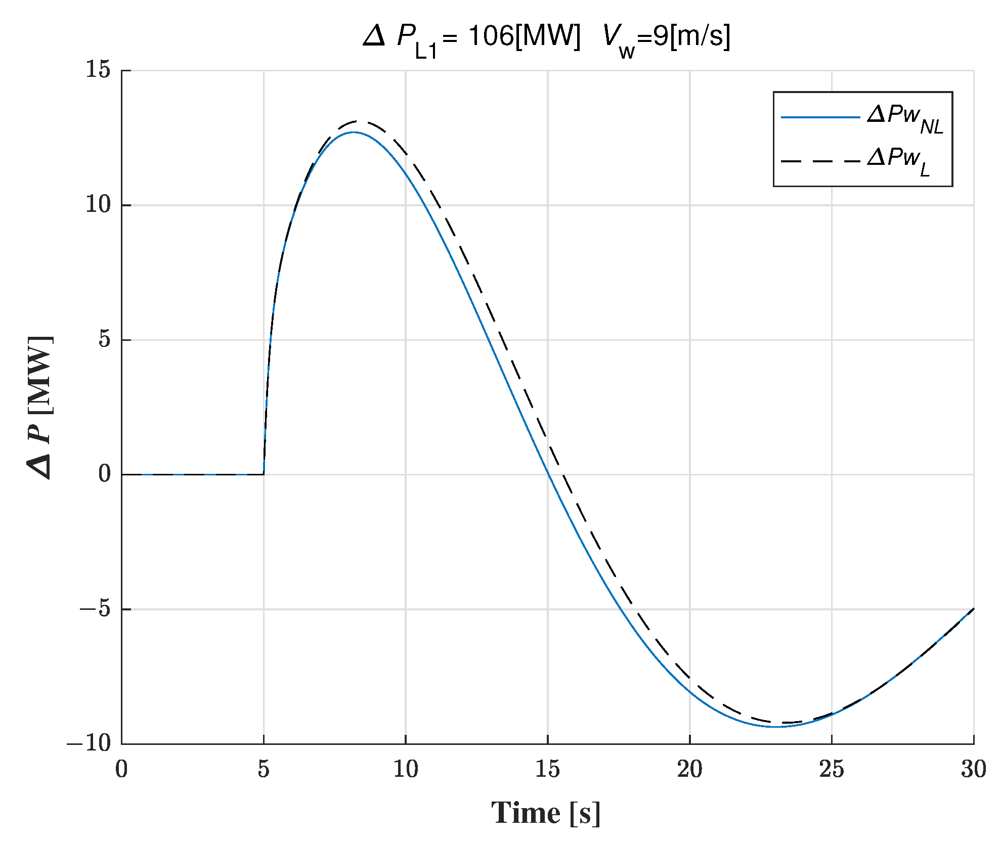
2.4. Validation of Wind Power Dynamics Linearization

The response of the synthetic inertia power output was simulated using Matlab-Simulink for both the nonlinear dynamic equations (16) and the linear model (17) for a power imbalance of 106 MW occurring in area-1. The comparison between the linear VSWT model and the non-linear VSWT model is presented in Figure 5, which demonstrates an adequate correspondence between them, where the RMS error between the curves is 3.03% compared to the maximum power value.

3. Study Case

The two-area power system was constructed using two one-machine equivalents of the Chilean power system connected through a transmission line, shown in Figure 6. The equivalent line reactance is denoted as $X_{12}$ in the same figure. As mentioned above, the parameter $K_{12}$ is associated with $X_{12}$ through (1).

The system parameters for each area shown in

Table 1. Power system parameters (source: Parameter identification from PMU measurements in Chilean Electric System, 2018–2020).

No.	$\mathbf{\Delta }{\mathit{P}}_{\mathit{L}}$	Load	${\mathit{K}}_{\mathit{c}}$	${\mathit{K}}_{\mathit{G}}$	H	${\mathit{T}}_{\mathit{a}}$	${\mathit{T}}_{\mathit{c}}$
	[MW]	[MW]	[GWs]	[$\frac{\mathbf{MW}}{\mathbf{Hz}}$]	[$\frac{\mathbf{MWs}}{\mathbf{Hz}}$]	[s]	[s]
1	128.0	7154.2	70.1	2088.0	2804.0	12.0	0.96
2	152.0	6963.1	65.5	1617.5	2620.0	18.8	3.19
3	190.0	7132.1	85.6	2286.9	3426.4	11.8	0.69
4	320.0	8693.1	104.3	1461.6	4172.0	17.4	1.24
5	480.0	7507.6	116.3	1866.6	4652.8	14.7	1.83
6	320.0	7619.9	85.1	1202.0	3402.0	4.5	0.04
7	120.0	6774.3	67.2	949.0	2689.6	94.9	6.52
8	194.0	6070.7	46.6	1420.0	1862.4	14.6	2.80
9	374.0	6836.4	57.4	843.9	2296.4	13.3	2.97
10	70.0	6179.4	20.6	691.6	822.4	32.7	6.28
11	140.0	7627.3	65.5	1949.1	2619.6	26.4	4.30
12	146.0	7627.3	62.9	1939.0	2516.8	25.1	4.68
13	132.0	7260.7	53.4	2002.1	2136.0	20.2	3.25
14	153.0	7242.6	93.0	2960.4	3720.8	26.9	5.36
15	224.0	7613.3	101.0	1735.7	4040.0	9.5	1.13
16	195.0	8697.8	59.9	1484.5	2395.2	14.7	2.67
17	160.0	7350.4	77.3	1507.4	3090.8	4.5	0.59
18	170.0	7239.0	84.6	1403.5	3385.2	18.6	3.84
19	106.0	5255.9	55.4	1168.5	2217.6	8.5	1.59
20	260.0	6862.1	39.8	1600.4	1590.4	15.4	3.83
21	190.0	4542.8	64.6	18.7	2583.2	87.4	4.88
22	116.0	8252.4	48.3	1921.0	1932.4	21.2	4.81

were obtained using an identification algorithm of the data of the power system using the Matlab System Identification Toolbox. The input of the algorithm are the initial values of the model parameters. For example, the initial values of the kinetic energy of rotating machines, $K_c$, and the governor droop, $K_G$, are estimated from the frequency data, using the oscillation equation of the power system, as explained in [22]. Data acquisition was carried out between 2018 and 2020, from phasor measurement units (PMU), located in the north and south of the Chile.

These frequency events were caused by power imbalances $\mathrm{\Delta }{P}_L$, also shown in the same table.

Integrating wind power dynamics and state feedback control in the reduced model presented in Figure 2, the block diagram shown in Figure 7 is obtained, where:

$$\begin{array}{cc}\hfill N_1\left(s\right)& =\frac{-1}{G{}_{f_1}\left(s\right)+G{}_{p{m}_1}\left(s\right)G_1\left(s\right)K{}_{G_1}-G_1\left(s\right)K{}_{G_i}-s{H}_i},\hfill \\ \hfill N_2\left(s\right)& =\frac{1}{G{}_{f_2}\left(s\right)+G{}_{p{m}_2}\left(s\right)G_2\left(s\right)K{}_{G_2}-G_2\left(s\right)K{}_{G_i}-s{H}_i},\hfill \end{array}$$

(37)

are the transfer function from $-\mathrm{\Delta }{P}_{12}$ to $\mathrm{\Delta }\overline{f_1}$ and $\mathrm{\Delta }\overline{f_2}$, respectively.

Additionally, in (37), $G_{f_i}\left(s\right)$, and $G_{p{m}_i}\left(s\right)$ are the transfer function between $\mathrm{\Delta }{f}_i$ to $\mathrm{\Delta }{P}_{w_i}$ and $\mathrm{\Delta }{P}_{m_i}$ to $\mathrm{\Delta }{P}_{w_i}$, respectively, when $i=1,2$.

The overall transfer function in Figure 7 is:

$${\displaystyle \frac{\mathrm{\Delta }\overline{f_1}-\mathrm{\Delta }\overline{f_2}}{-\mathrm{\Delta }{P}_{12}}}={\displaystyle \frac{\mathrm{\Delta }\overline{f_1}}{-\mathrm{\Delta }{P}_{12}}}-{\displaystyle \frac{\mathrm{\Delta }\overline{f_2}}{-\mathrm{\Delta }{P}_{12}}}=N_1\left(s\right)-N_2\left(s\right)=M\left(s\right),$$

(38)

and its equivalent block diagram in the Laplace domain is shown in Figure 8.

Global stability is analyzed using the root locus plot of $M\left(s\right)/s$, considering a negative feedback SISO system, as was explained in [31]. Different scenarios by combining high and low inertia in each area were developed, and the simulations were performed using Matlab-Simulink.

3.1. State Feedback Gains

The proportional state feedback gains calculated using (29) for the study cases are presented in

Table 2. Proportional state feedback gain parameters calculated using (29).

Figure	${\mathit{K}}_1$	${\mathit{K}}_2$
Figure 9 and Figure 10	[0.0987 −0.0008 0.3677 −0.4309]	[−0.1044 −0.0006 0.3312 −0.5065]
Figure 11 and Figure 12		[−0.1977 −0.0070 0.7150 −0.3407]

.

3.2. Quadratic Performance Index Matrices

The following are matrices of the performance index (20) used in the study case, which were obtained through a sensitivity analysis.

$$R_1=R_2=0.2;Q_1=Q_2=\left[\begin{array}{cccc}1& 0& 0& 0\\ 0& 1\times {10}^{-9}& 0& 0\\ 0& 0& 1\times {10}^{-9}& 0\\ 0& 0& 0& 1\times {10}^{-9}\end{array}\right].$$

Without loss of generality, the system input is $\mathrm{\Delta }{P}_{L_2}$, with $\mathrm{\Delta }{P}_{L_1}=0$.

4. Results

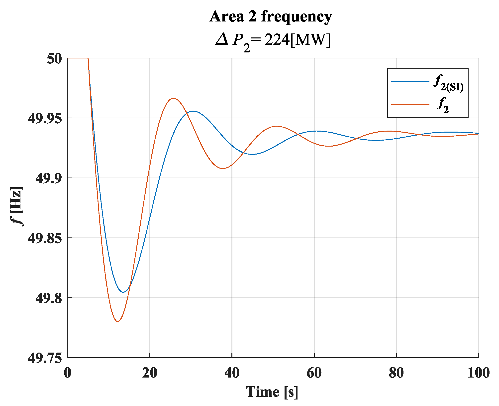
4.1. Frequency Response

Figure 9 represents a comparison between the frequency response of area-1 and area-2, with respect to a power imbalance of 224 MW applied in area-2. Both areas have high rotating inertia, with $H_1$ = 4652.8 and $H_2$ = 4040 [MWs/Hz] corresponding to Nos. 5 and 15 of Table 1, respectively. It is observed that the frequencies converge to the same value after 100 s.

Figure 10 illustrates the impact of the SI control on the frequency of area-2 for the same power imbalance presented in Figure 9. It is evident that the implementation of SI control has a positive effect on reducing the frequency Nadir and the RoCoF.

Figure 11 displays a scenario where the inertia of area-1 remains high at $H_1$ = 4652.8 MWs/Hz, whereas the inertia of area-2 is low, with $H_2$ = 1862 MWs/Hz, corresponding to No. 5 and 8 of Table 1, respectively. For comparison purposes, the same power imbalance as Figure 9 and Figure 10 was considered.

Similarly to Figure 10, in Figure 12, the effect of SI control on the frequency response of area-2 is shown. As this area has lower inertia, a greater influence of SI control is observed in improving the RoCoF and Nadir indicators.

4.2. Performance Indicators

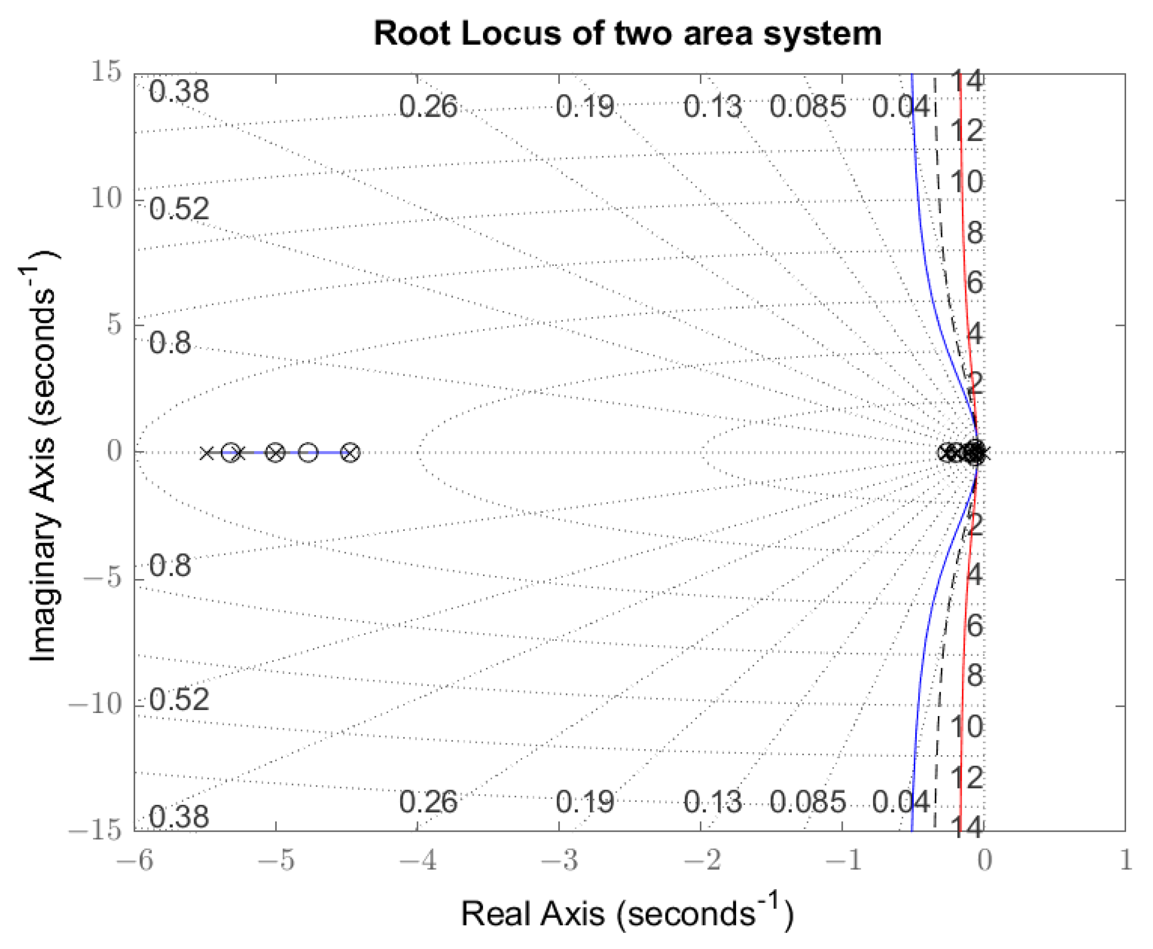
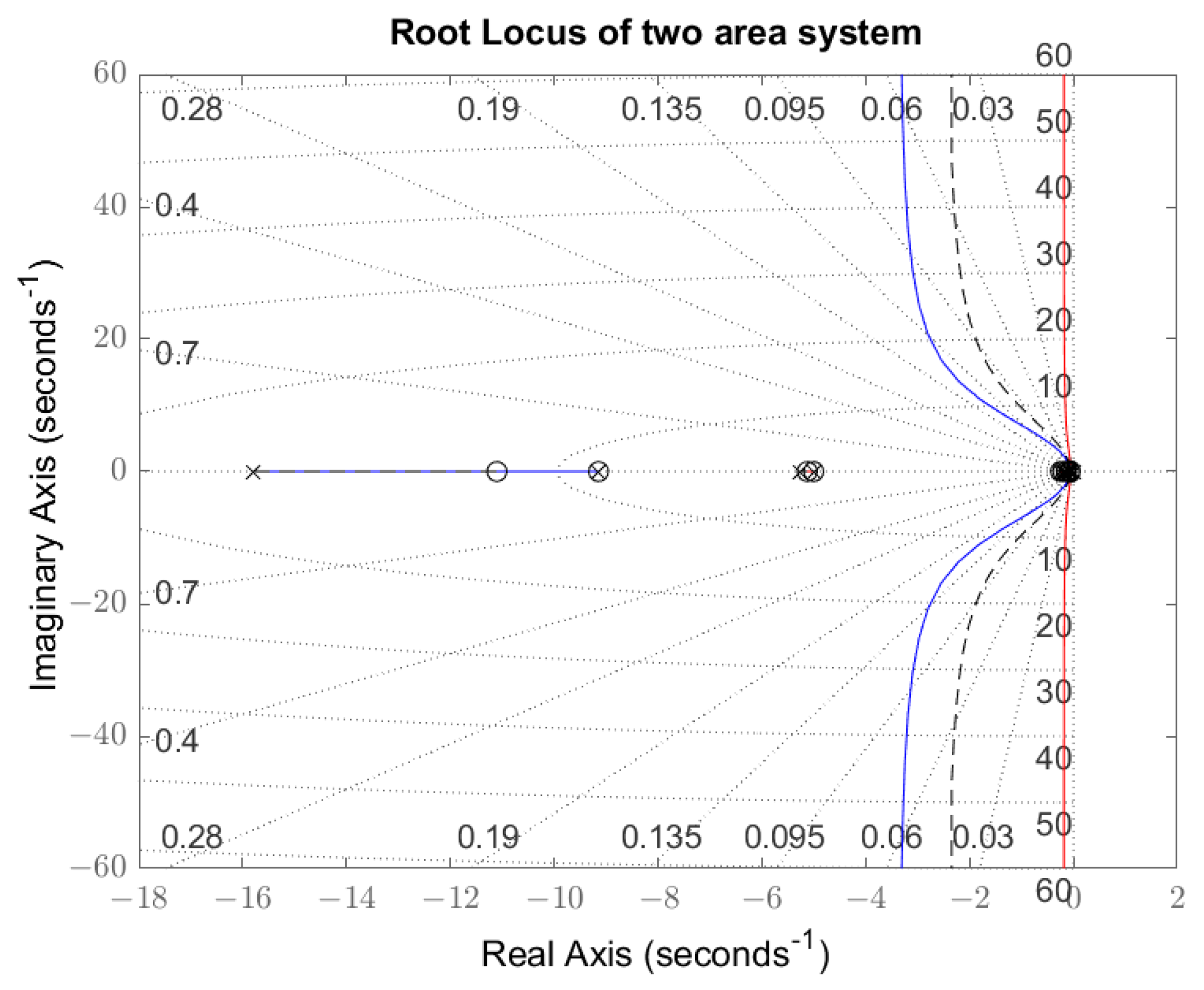
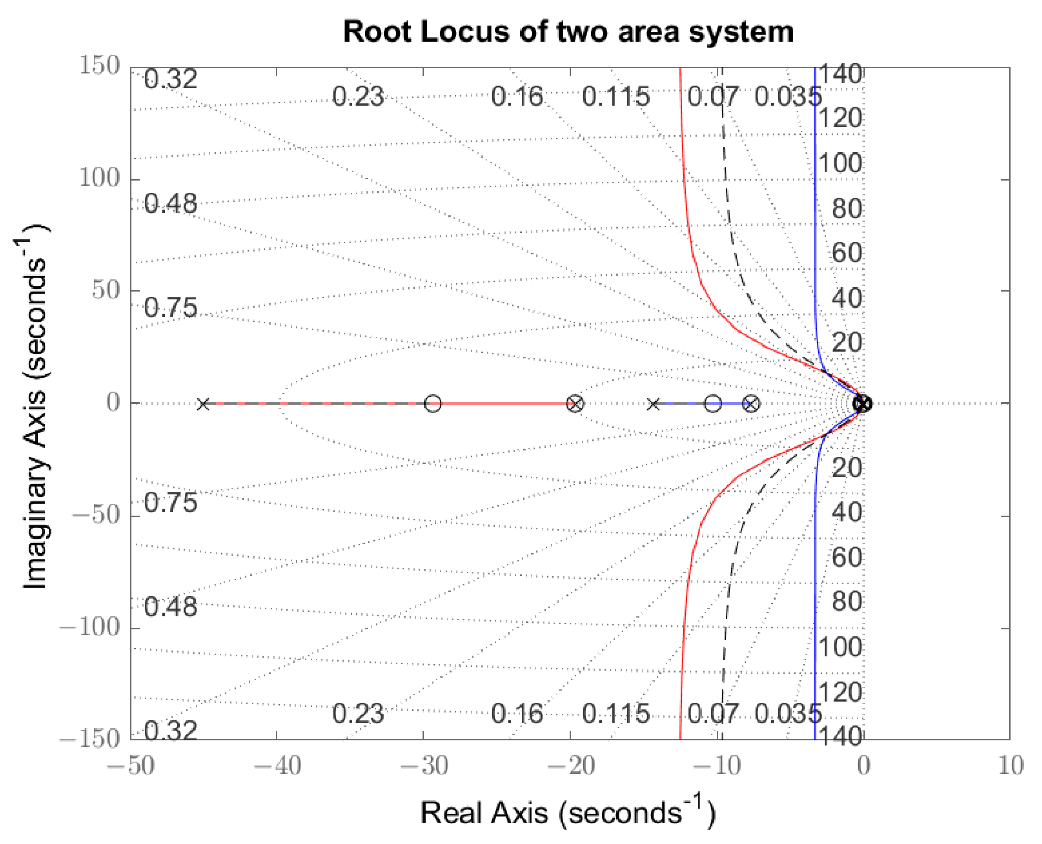
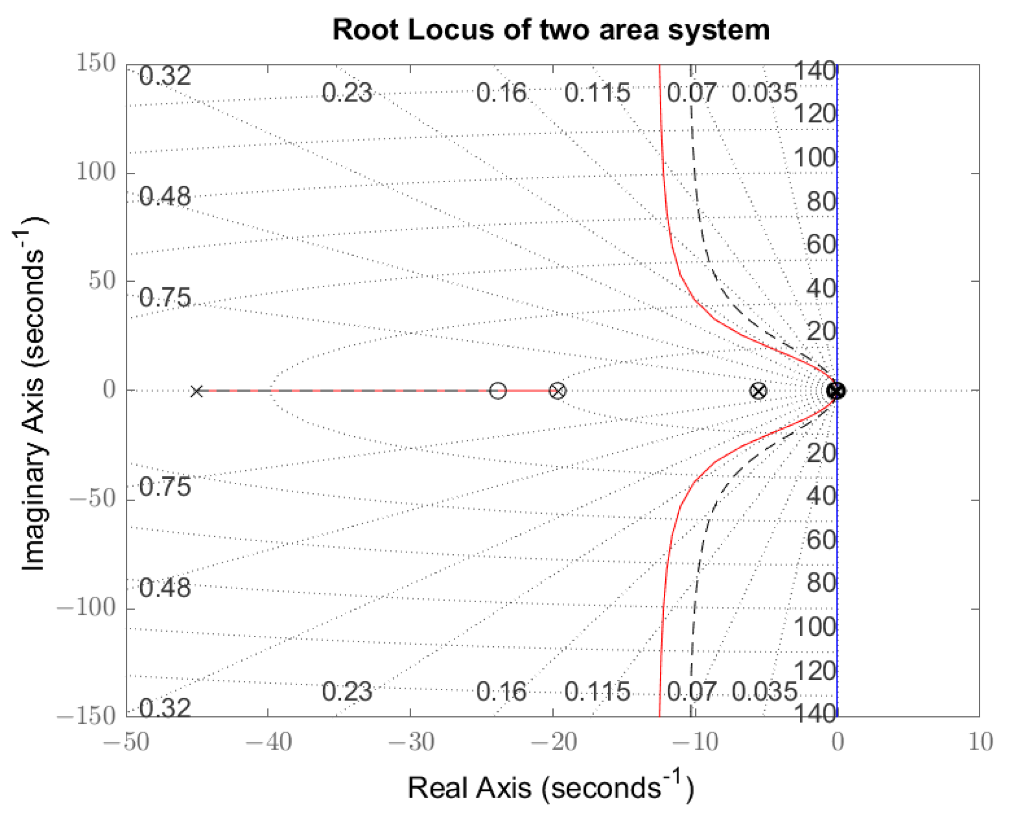
The RoCoF and Nadir indicators calculated for the case shown in Figure 10 are presented in

Table 3. Simulation-derived SI control performance indicators obtained from data in Figure 10.

Indicator	No Control	SI Control	$\mathbf{\Delta }$%
RoCoF [Hz/s]	−0.0554	−0.0551	−0.5183
Nadir [Hz]	49.780	49.804	+0.050

.

The performance indicators of Figure 12 are presented in

Table 4. Simulation-derived SI control performance indicators obtained from data in Figure 12.

Indicator	No Control	SI Control	$\mathbf{\Delta }$%
RoCoF [Hz/s]	−0.1202	−0.1164	−3.1400
Nadir [Hz]	49.680	49.740	+0.128

.

4.3. Root Locus

As explained above, the root locus plot of $M\left(s\right)/s$ is shown in order to analyze the stability of the global system when $K_{12}$ varies. In the same figure, three cases are presented:

• case 1 in red, where both areas are equal, each one having an inertia $H_1$ varying between 822.4 and 4652.8 [MWs/Hz] and global transfer function $2·N_1\left(s\right)$;
• case 2 in blue, where both areas are equal, each one having an inertia $H_2$ varying between 1862.2 and 4040.0 [MWs/Hz] and global transfer function $2·N_2\left(s\right)$; and
• case 3 in dashed-black, where area-1 and area-2 are different, with values of total inertia between ${(H_1+H_2)}_{min}$ and ${(H_1+H_2)}_{max}$ and transfer function $|N_1\left(s\right)| + |N_2\left(s\right)|$.

5. Discussion

This work presents a methodological analysis of a two-area power system with wind power integration and SI control. The results provide important guidelines on how to deal with stability considering a broader application of SI in a more realistic scenario of a two-area system established as a duplicate of the Chilean national electric system.

5.1. Analysis of Results

5.1.1. Frequency Response

The impact of SI control is more significant when applied to a low-inertia area. This observation is evident in Table 4, which shows a reduction in RoCoF of 3.14% when the inertia in area-2 was low. By contrast, when the inertia in area-2 was high, only a 0.5% reduction in RoCoF was achieved, as indicated in Table 3. These findings highlight the potential contribution of SI control to improving frequency indicators within the power system. As expected from the control method used, the Nadir improvement is comparatively smaller than that of RoCoF.

5.1.2. Root-Locus

As expected, the effect of decreasing inertia moves the root locus plot to the left side of the plane (faster system); this can be observed by comparing the evolution of the red plot from Figure 13, Figure 14 and Figure 15 or Figure 16. The opposite occurs when inertia increases (slower system), as shown in the evolution of the blue plot between Figure 14 and Figure 15 or Figure 16. It can be seen that if $N_1\left(s\right)$ and $N_2\left(s\right)$ are stabilized in a decentralized way, the dynamic system resulting from the interconnection of both areas remains stable for all cases analyzed. This system is represented by the black dashed line in the root locus diagrams, and its location is between the two stable root locus plots of $N_1\left(s\right)$ and $N_2\left(s\right)$.

5.2. Advantages and Limitations of the Proposed Method

In terms of the proposed method, it offers several advantages in modeling a complex power system comprising two areas with wind power and synthetic inertia control, particularly for conducting stability analysis under varying interconnection links. A significant benefit of the data-driven model obtained is that it eliminates the need for extensive knowledge about the equipment’s parameters. However, there are certain limitations associated with the application of the proposed method. The analysis considered linear models for the dynamics of the power system, transmission links, and the dynamics of wind power. As a result, these models are valid within a limited domain around the equilibrium point.

5.3. Conclusions and Recommendations

The simulation results have shown that in a two-area power system with distinct parameters for each area, global stability can be accomplished by independently tuning the SI controllers in each area. This way, each SI control area can operate in a decentralized manner, reducing the complexity in communication software and hardware for a centralized solution and also reducing the time response of the control system.

The root locus method has proven to be a reliable method for assessing the stability of a two-area power system over a wide range of interconnection link variation, represented through the $K_{12}$ parameter.

The models of the two-area power system, wind power, and SI control can be used to analyze additional variables when incorporating new devices, such as DC links, power capacitors, solar generation, and others. However, it is important to consider the limitations of these models, as explained in Section 5.2.

5.4. Future Work

In large interconnected power systems, such as the European system, the existence of weak links between different power systems can result in inter-area electromechanical oscillations involving more than two areas. Addressing these inter-area oscillations among various groups presents a significant challenge for synthetic inertia control techniques, particularly in terms of ensuring global system stability. Consequently, future research will focus on studying the stability aspects of SI control when applied to multi-area power systems.

References

1. Agathokleous, C.; Ehnberg, J. A quantitative study on the requirement for additional inertia in the european power system until 2050 and the potential role of wind power. Energies 2020, 13, 2309. [Google Scholar] [CrossRef]
2. Ulbig, A.; Borsche, T.S.; Andersson, G. Impact of Low Rotational Inertia on Power System Stability and Operation; IFAC: Prague, Czech Republic, 2014; Volume 19, pp. 7290–7297. [Google Scholar] [CrossRef]
3. Kundur, P.; Paserba, J.; Ajjarapu, V.; Andersson, G.; Bose, A.; Canizares, C.; Hatziargyriou, N.; Hill, D.; Stankovic, A.; Taylor, C.; et al. Definition and classification of power system stability. IEEE Trans. Power Syst. 2004, 19, 1387–1401. [Google Scholar] [CrossRef]
4. Nguyen, H.T.; Yang, G.; Nielsen, A.H.; Jensen, P.H. Combination of synchronous condenser and synthetic inertia for frequency stability enhancement in low-inertia systems. IEEE Trans. Sustain. Energy 2019, 10, 997–1005. [Google Scholar] [CrossRef]
5. Li, Q.; Ren, B.; Tang, W.; Wang, D.; Wang, C.; Lv, Z. Analyzing the inertia of power grid systems comprising diverse conventional and renewable energy sources. Energy Rep. 2022, 8, 15095–15105. [Google Scholar] [CrossRef]
6. Rapizza, M.R.; Canevese, S.M. Fast frequency regulation and synthetic inertia in a power system with high penetration of renewable energy sources: Optimal design of the required quantities. Sustain. Energy Grids Netw. 2020, 24, 100407. [Google Scholar] [CrossRef]
7. Fang, J.; Tang, Y.; Li, H.; Blaabjerg, F. The Role of Power Electronics in Future Low Inertia Power Systems. In Proceedings of the 2018 IEEE International Power Electronics and Application Conference and Exposition (PEAC), Shenzhen, China, 4–7 November 2018; pp. 1–6. [Google Scholar] [CrossRef]
8. Ratnam, K.S.; Palanisamy, K.; Yang, G. Future low-inertia power systems: Requirements, issues, and solutions—A review. Renew. Sustain. Energy Rev. 2020, 124, 109773. [Google Scholar] [CrossRef]
9. Dreidy, M.; Mokhlis, H.; Mekhilef, S. Inertia response and frequency control techniques for renewable energy sources: A review. Renew. Sustain. Energy Rev. 2017, 69, 144–155. [Google Scholar] [CrossRef]
10. Bonfiglio, A.; Invernizzi, M.; Labella, A.; Procopio, R. Design and Implementation of a Variable Synthetic Inertia Controller for Wind Turbine Generators. IEEE Trans. Power Syst. 2019, 34, 754–764. [Google Scholar] [CrossRef]
11. Riquelme, E.; Fuentes, C.; Chavez, H. A review of limitations of wind synthetic inertia methods. In Proceedings of the 2020 IEEE PES Transmission and Distribution Conference and Exhibition—Latin America, T and D LA, Montevideo, Uruguay, 28 September–2 October 2020. [Google Scholar] [CrossRef]
12. Pelletier, M.; Phethean, M.; Nutt, S. Grid code requirements for artificial inertia control systems in the New Zealand power system. In Proceedings of the 2012 IEEE Power and Energy Society General Meeting, San Diego, CA, USA, 22–26 July 2012; IEEE: Piscataway, NJ, USA, 2012; pp. 1–7. [Google Scholar]
13. Brisebois, J.; Aubut, N. Wind farm inertia emulation to fulfill Hydro-Québec’s specific need. In Proceedings of the 2011 IEEE Power and Energy Society General Meeting, Detroit, MI, USA, 24–29 July 2011; pp. 1–7. [Google Scholar] [CrossRef]
14. Massaro, F.; Musca, R.; Vasile, A.; Zizzo, G. A simulation study for assessing the impact of energy storage systems for Fast Reserve with additional synthetic inertia control on the Continental Europe synchronous area. Sustain. Energy Technol. Assessm. 2022, 53, 102763. [Google Scholar] [CrossRef]
15. Grebe, E.; Kabouris, J.; López Barba, S.; Sattinger, W.; Winter, W. Low frequency oscillations in the interconnected system of Continental Europe. In Proceedings of the IEEE PES General Meeting, Minneapolis, MN, USA, 25–29 July 2010; pp. 1–7. [Google Scholar] [CrossRef]
16. Mohamed, T.H.; Bevrani, H.; Hassan, A.A.; Hiyama, T. Decentralized model predictive based load frequency control in an interconnected power system. Energy Convers. Manag. 2011, 52, 1208–1214. [Google Scholar] [CrossRef]
17. Ojaghi, P.; Rahmani, M. LMI-Based Robust Predictive Load Frequency Control for Power Systems with Communication Delays. IEEE Trans. Power Syst. 2017, 32, 4091–4100. [Google Scholar] [CrossRef]
18. Tabassum, F.; Rana, M.S. Robust Control of Frequency for Multi-Area Power System. In Proceedings of the 2020 IEEE Region 10 Symposium (TENSYMP), Dhaka, Bangladesh, 5–7 June 2020; pp. 86–89. [Google Scholar] [CrossRef]
19. Raj, T.D.; Kumar, C.; Kotsampopoulos, P.; Fayek, H.H. Load Frequency Control in Two-Area Multi-Source Power System Using Bald Eagle-Sparrow Search Optimization Tuned PID Controller. Energies 2023, 16, 2014. [Google Scholar] [CrossRef]
20. Kumar Maurya, A.; Khan, H.; Ahuja, H. Stability Control of Two-Area of Power System Using Integrator, Proportional Integral and Proportional Integral Derivative Controllers. In Proceedings of the 2023 International Conference on Artificial Intelligence and Smart Communication (AISC), Greater Noida, India, 27–29 January 2023; pp. 273–278. [Google Scholar] [CrossRef]
21. Ma, M.; Zhang, C.; Shao, L.; Sun, Y. Primary frequency regulation for multi-area interconnected power system with wind turbines based on DMPC. In Proceedings of the Chinese Control Conference, CCC. IEEE Computer Society, Chengdu, China, 27–29 July 2016; Volume 2016, pp. 4384–4389. [Google Scholar] [CrossRef]
22. Riquelme, E.; Chavez, H.; Barbosa, K.A. RoCoF-Minimizing H Norm Control Strategy for Multi-Wind Turbine Synthetic Inertia. IEEE Access 2022, 10, 18268–18278. [Google Scholar] [CrossRef]
23. Yedrzejewski, N.; Giusto, A. Potential impact of wind-based Synthetic Inertia on the Frequency Response of the Argentine-Uruguayan Interconnected Power Systems. In Proceedings of the 2022 IEEE PES Innovative Smart Grid Technologies—Asia (ISGT Asia), Auckland, New Zealand, 21–24 November 2023; pp. 505–509. [Google Scholar] [CrossRef]
24. Roy, N.K.; Islam, S.; Podder, A.K.; Roy, T.K.; Muyeen, S.M. Virtual Inertia Support in Power Systems for High Penetration of Renewables—Overview of Categorization, Comparison, and Evaluation of Control Techniques. IEEE Access 2022, 10, 129190–129216. [Google Scholar] [CrossRef]
25. Adu, J.A.; Tossani, F.; Pontecorvo, T.; Ilea, V.; Vicario, A.; Conte, F.; D’Agostino, F. Coordinated Inertial Response Provision by Wind Turbine Generators: Effect on Power System Small-Signal Stability of the Sicilian Network. In Proceedings of the 2022 IEEE International Conference on Environment and Electrical Engineering and 2022 IEEE Industrial and Commercial Power Systems Europe (EEEIC/I&CPS Europe), Prague, Czech Republic, 28 June–1 July 2022; pp. 1–6. [Google Scholar] [CrossRef]
26. Kundur, P.; Balu, N.J.; Lauby, M.G. Power System Stability and Control; The EPRI Power System Engineering Series; McGraw-Hill: New York, NY, USA, 1994. [Google Scholar]
27. Anderson, P.M.; Mirheydar, M. A low-order system frequency response model. IEEE Trans. Power Syst. 1990, 5, 720–729. [Google Scholar] [CrossRef]
28. Chávez, H.; Hezamsadeh, M.R.; Carlsson, F. A simplified model for predicting primary control inadequacy for nonresponsive wind power. IEEE Trans. Sustain. Energy 2016, 7, 271–278. [Google Scholar] [CrossRef]
29. Liu, Y.z.; Zhao, D.w.; Zhang, L.; Zhu, L.z.; Chen, N. Simulation study on transient characteristics of DFIG wind turbine systems based on dynamic modeling. In Proceedings of the 2014 China International Conference on Electricity Distribution (CICED), Shenzhen, China, 23–26 September 2014; pp. 1408–1413. [Google Scholar] [CrossRef]
30. Duan, G.R.; Yu, H.H. LMIs in Control Systems: Analysis, Design and Applications, 2nd ed.; CRC Press: Boca Raton, FL, USA, 2013. [Google Scholar]
31. Tan, W. Tuning of PID load frequency controller for power systems. Energy Convers. Manag. 2009, 50, 1465–1472. [Google Scholar] [CrossRef]
Figure 1. Two-area power system with variable interconnection link and SI control.
Processes 11 02488 g001
Figure 2. Two-area power system reduced model for frequency response.
Processes 11 02488 g002
Figure 3. One-mass VSWT model.
Processes 11 02488 g003
Figure 4. Dynamic interactions.
Processes 11 02488 g004
Figure 5. Comparison of synthetic inertia power output: continuous line represents the linear model, and dashed line represents the non-linear model.
Processes 11 02488 g005
Figure 6. Two-area power system used for study case.
Processes 11 02488 g006
Figure 7. Two-area power system with wind power integration in Laplace domain.
Processes 11 02488 g007
Figure 8. Equivalent two-area system with wind power integration in Laplace domain.
Processes 11 02488 g008
Figure 9. Simulation illustrating the frequency response for two-area power system with H 1 = 4652.8 and H 2 = 4040 [MWs/Hz].
Processes 11 02488 g009
Figure 10. Simulation illustrating the effect of SI control on frequency response, with H 1 = 4652.8 and H 2 = 4040 [MWs/Hz].
Processes 11 02488 g010
Figure 11. Simulation depicting the frequency response for two-area power system with H 1 = 4652.8 and H 2 = 1862.0 [MWs/Hz].
Processes 11 02488 g011
Figure 12. Simulation illustrating the effect of SI control on frequency response, with H 1 = 4652.8 and H 2 = 1862.0 [MWs/Hz].
Processes 11 02488 g012
Figure 13. Root locus simulation with H 1 = 4652.8 and H 2 = 4040.0 [MWs/Hz].
Processes 11 02488 g013
Figure 14. Root locus simulation with H 1 = 4652.8 and H 2 = 1862.0 [MWs/Hz].
Processes 11 02488 g014
Figure 15. Root locus simulation with H 1 = 822.4 and H 2 = 1932.4 [MWs/Hz].
Processes 11 02488 g015
Figure 16. Root locus simulation with H 1 = 822.4 and H 2 = 4172.0 [MWs/Hz].
Processes 11 02488 g016