
Rotating Machinery Fault Diagnosis under Time–Varying Speed Conditions Based on Adaptive Identification of Order Structure

1
School of Mechanical Engineering, University of Science and Technology Beijing, Beijing 100083, China
2
China North Vehicle Research Institute, Beijing 100072, China
*
Author to whom correspondence should be addressed.
Processes 2024, 12(4), 752; https://doi.org/10.3390/pr12040752
Submission received: 16 March 2024
/
Revised: 2 April 2024
/
Accepted: 4 April 2024
/
Published: 8 April 2024
(This article belongs to the Special Issue Industrial IoT-Enabled Modeling and Optimization for the Process Industry)
Abstract
:Rotating machinery fault diagnosis is of key significance for ensuring safe and efficient operation of various industrial equipment. However, under nonstationary operating conditions, the fault–induced characteristic frequencies are often time–varying. Conventional Fourier spectrum analysis is not suitable for revealing time–varying details, and nonstationary fault feature extraction methods are still in desperate need. Order spectrum can reveal the rotational–speed–related time–varying frequency components as spectral peaks in order domain, thus facilitating fault feature extraction under time–varying speed conditions. However, the speed–unrelated frequency components are still nonstationary after angular–domain resampling, thus causing wide–band features and interferences in the order spectrum. To overcome such a drawback, this work proposes a rotating machinery fault diagnosis method based on adaptive separation of time–varying components and order feature extraction. Firstly, the rotational speed is estimated by the multi–order probabilistic approach (MOPA), thus eliminating the inconvenience of installing measurement equipment. Secondly, adaptive separation of the time–varying frequency component is achieved through time–varying filtering and surrogate test. It effectively eliminates interference from irrelevant components and noise. Finally, a high–resolution order spectrum is constructed based on the average amplitude envelope of each mono–component. It does not involve Fourier transform or angular–domain resampling, thus avoiding spectral leakage and resampling errors. By identifying the fault–related spectral peaks in the constructed order spectrum, accurate fault diagnosis can be achieved. The Rényi entropy values of the proposed order spectrum are significantly lower than those of the traditional order spectrum. This result verifies the effective energy concentration and high resolution of the proposed order spectrum. The results of both numerical simulation and lab experiments confirm the effectiveness of the proposed method in accurately presenting the time–varying frequency components for rotating machinery diagnosing faults.
1. Introduction
Rotating machineries are prone to fault under harsh environment and complex operating conditions. Undetected failures may deteriorate the accuracy and/or efficiency of the equipment, or even cause safety accidents. Thus, rotating machinery fault diagnosis is of key significance. Fault feature extraction from the measured signals, e.g., vibration, sound, and current, enables accurate fault detection and diagnosis [1,2,3,4,5,6], yet most efforts are based on the assumption of fixed operating conditions. Rotating machinery fault diagnosis under nonstationary operating conditions still deserves deep research.
In engineering practice, rotating machinery often operates under time–varying speed and/or load conditions, which are referred to as nonstationary operating conditions. Consequently, the frequency and/or amplitude of vibration signals undergo corresponding changes with varying operational conditions, disabling effective fault feature extraction in the frequency domain. To address this issue, researchers have tried to map the time–varying frequency details into a constant one [7,8,9,10]. Such an approach transforms the three–dimensional time–frequency features into two–dimensional spectral features, enabling more intuitive and convenient identification of nonstationary characteristics. It is capable of handling time–varying and multicomponent signals; thus, it is promising for rotating machinery fault diagnosis under nonstationary operating conditions.
Order tracking (OT) realizes this concept by resorting time–domain signals according to fixed angular increments, effectively converting time–varying frequency into constant frequency [7]. OT methods can be broadly classified into three categories: hardware order tracking (HOT), computed order tracking (COT), and tacholess order tracking (TOT) [8,9]. HOT adjusts the sampling frequency proportionally to the rotational speed via hardware control. It offers real–time angular–domain sampling [10], yet delays and errors may occur during rapid speed changes [11]. Additionally, the reliance on extra hardware components increases system complexity and cost. COT resamples the measured time–domain signal into an angular domain on a digital platform [12], and the order spectrum is generated by performing Fourier transform on the angular–domain signal. However, the angular–domain resampling needs to be guided by the precise instantaneous rotational speed. The acquisition of rotational speed typically relies on an extra tachometer, which can be available in real applications. To eliminate the need for an external tachometer, researchers have proposed the TOT method. It aims at estimating the instantaneous speed based on the signal itself [13]. Researchers have explored various methods for estimating rotational speed from vibration signals, including Hilbert–transform–based phase demodulation [14], iterative phase demodulation based on angular resampling [15], and the Teager–Kaiser energy operator [16]. However, these methods still face challenges, such as the presence of multiple harmonic modes in the vibration signal, interactions between rotational frequency harmonics and mechanical structure resonances, and low signal–to–noise ratios, which can lead to errors in instantaneous speed estimation. To address these issues, the multi–order probabilistic approach (MOPA) [17] has been proposed for tracking instantaneous speed. MOPA regards the instantaneous spectrum as a probability density function of instantaneous speed and estimates the speed based on the prior continuity of the function. Recent studies have demonstrated the effectiveness of MOPA in various applications [18,19,20].
In addition, while order spectrum is effective in identifying time–varying frequency components related to rotational speed in nonstationary conditions [21,22], components unrelated to rotational speed, such as resonances and background noise, are still nonstationary in angular domain. Their energy is not concentrated at a specific order, and result in wide–band feature. Such a result may lead to the misidentification of meaningful order components, hindering effective fault feature extraction. To address this issue, various techniques have been proposed, such as Vold–Kalman filtering [23] and phase–demodulation–based order tracking [24]. However, these methods often rely on prior knowledge of the targeted instantaneous frequency, and cannot distinguish interferences caused by speed–unrelated components from the noises.
In addition to OT, alternative approaches have been proposed for achieving order tracking objectives. One such method, introduced by Blough and Brown [25], involves modifying the Fourier transform kernel to extract order domain information directly from time–domain signals. Borghesani [26] proposed a speed–synchronized discrete Fourier transform, in which the modified Fourier transform kernel is characterized by instantaneous rotational speed, eliminating the need for resampling and interpolation steps. While this approach avoids resampling and interpolation errors associated with COT methods, it still suffers from spectral blurring caused by the nonstationarity of amplitude envelopes. Researchers have also proposed various techniques aimed at reducing spectral aliasing and spectral leakage [27,28,29,30]. However, these methods still do not eliminate spectral blurring fundamentally due to the nonstationarity of amplitude envelopes in time–varying conditions.
In this paper, we propose a novel rotating machinery fault diagnosis method, based on adaptive separation of time–varying components and order spectrum analysis. The objectives of the proposed method are as follows:
- Avoid the inconvenience and error of speed measurement.
The proposed method introduces MOPA to directly extract instantaneous rotational speed from the signal without external tachometer.
- Eliminate the interference of irrelevant components and noise.
It effectively separates time–varying components using a combination of time–varying filtering and surrogate test, eliminating interferences from irrelevant components and background noise.
- Avoid spectral energy leakage and achieve fine resolution.
The order spectrum is directly constructed by the average amplitude envelope of each individual order component, thus avoiding spectral energy leakage during Fourier transform and achieving fine resolution. The achieved precise revelation of fault–related order components enables effective fault diagnosis of rotating machinery under nonstationary operating conditions.
The remainder of this article is structured as follows. Section 2 details the proposed fault diagnosis method, including accurate acquisition of instantaneous rotational speed, adaptive separation of time–varying components, elimination of irrelevant components and noise, and precise identification of frequency orders. Section 3 demonstrates the effectiveness of the proposed method through an analysis of time–varying multicomponent simulation signals. Section 4 further validates the effectiveness of the proposed method in diagnosing rolling–element–bearing faults via laboratory experiments. Finally, Section 5 concludes the paper.
2. The Proposed Fault Diagnosis Method
2.1. Estimation of Instantaneous Rotational Speed
Under nonstationary operating conditions, the vibration components of critical components exhibit time–varying characteristics, and their instantaneous frequencies are closely related to rotational speed. Therefore, in the process of extracting time–varying components, instantaneous rotational speed serves as indispensable prior knowledge, providing an important basis for subsequent component identification and ridge extraction. The accurate estimation of instantaneous rotational speed thus becomes a crucial step in the entire signal processing workflow. In practical engineering applications, the acquisition of rotational speed typically relies on specific hardware devices, such as tachometers or encoders. However, the introduction of these devices not only increases additional costs but also poses various inconveniences during actual installation and use. To effectively address this issue, researchers have focused on directly extracting instantaneous rotational speed information from the vibration signal itself, eliminating the need for external measurement instruments.
In this context, methods for extracting rotational speed information by tracking harmonics in the time–frequency representation of vibration signals have emerged. Among them, MOPA has been widely used in various signal processing scenarios due to its high accuracy and excellent robustness in rotational speed identification.
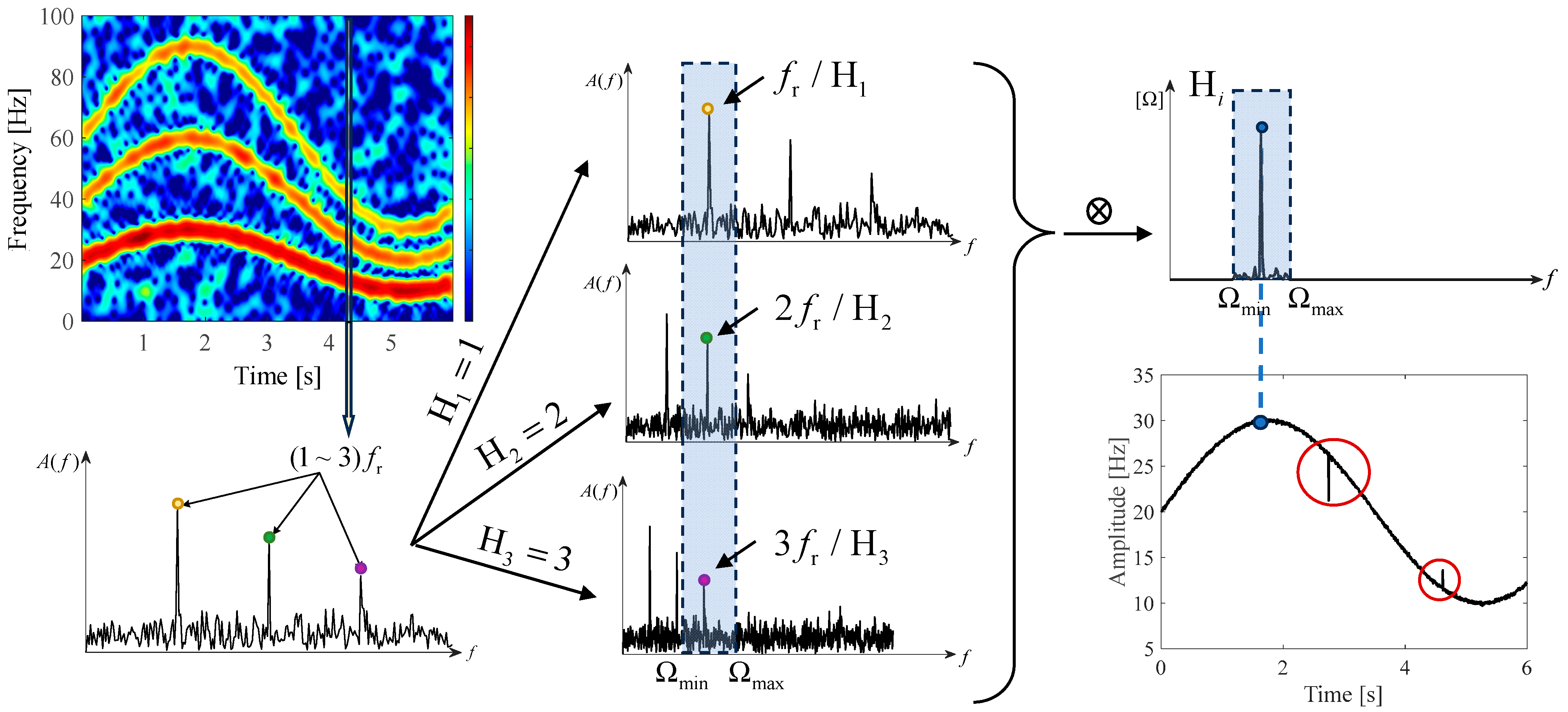
Rotating machinery vibrations are usually dominated by the rotating frequency and its harmonics. The higher the spectral amplitude at a frequency of a harmonic order , the more likely it is that the rotating frequency will be equal to the frequency divided by the harmonic order . Therefore, combining multiple harmonic components can effectively enhance noise resistance performance. Motivated by this fact, MOPA regards the instantaneous spectrum at each moment as a probability density function (PDF) of instantaneous rotational speed and accurately estimates the instantaneous rotational speed based on the prior continuity of the PDF, as shown in Figure 1. The specific procedure is as follows.
Firstly, to mitigate the impact of structural modal responses on the instantaneous spectral amplitude of rotational frequency harmonics, construct a whitened time–frequency representation and regard each column as the instantaneous spectrum at each time instance.
Then, generate the PDF by scaling the instantaneous spectrum with all known harmonic orders , maximum speed , and minimum speed :
where is the upper frequency limit and is a normalization factor. Multiply PDFs of all orders to yield a global PDF:
Next, taking into account the inertia effects of actual mechanical systems, changes in instantaneous rotational speed should be continuous without any step changes. To ensure the continuity of the probability density function, a Gaussian function is introduced as a smoothing process. Perform a priori continuity to smooth the global PDF . For any time instance , the PDF can be estimated by convolving a neighboring PDF with a centered Gaussian [17]:
where is a variance and the priori continuity is
As the variance of the Gaussian function increases, the smoothing effect of convolution also increases accordingly. Multiply PDFs including a priori continuity to yield a smoothed PDF:
Finally, the frequencies corresponding to the maximum values at each moment are extracted from the smoothed PDFs. By fitting the relationship between these frequency values and time, an accurate estimation of instantaneous rotational speed is achieved.
2.2. Adaptive Separation of Time–Varying Components
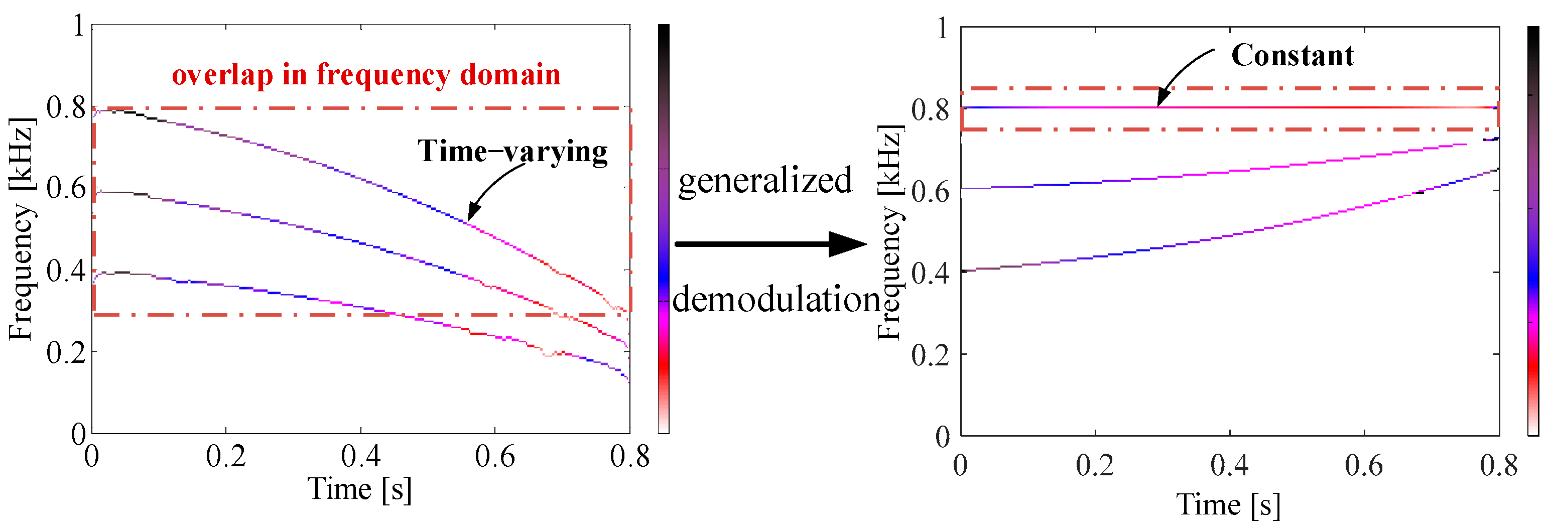
For nonstationary signals, due to the time–varying nature of their sidebands, frequency domain overlap often occurs among various components, making effective separation challenging. As shown in the left figure of Figure 2, there is frequency domain overlap among the components. If filtering is performed directly, it will result in truncation of the time–varying frequencies. To address this issue and ensure the integrity of component extraction, time–varying filtering can be utilized for complete component extraction. The core idea of the time–varying component extraction method based on time–varying filtering is as follows.
According to prior knowledge of instantaneous rotational speed , the instantaneous frequency of the kth order harmonic component in the time–frequency domain is calculated as . To achieve complete extraction of components, generalized demodulation is employed to convert time–varying frequency components into constant frequency components, as shown in the right figure of Figure 2. Specifically speaking, the signal is multiplied with a generalized demodulation function to convert the kth order harmonic component into a constant frequency component
where . In this case, the constant frequency components do not overlap with other components in the frequency domain, facilitating their separation through filtering operations.
Then, the component of constant frequency is separated by filtering, and the component is multiplied with the inverse generalized demodulation function to restore the original component by
However, the instantaneous frequencies of the rotational frequency harmonic components do not change at the same rate. Specifically, the higher the harmonic order, the greater the rate of change in its instantaneous frequency. This means that during a single generalized demodulation process, only one target component can be converted into a constant frequency component, while other target components may still exhibit time–varying characteristics or even overlap in the frequency domain. To overcome this challenge, iterative application of generalized demodulation is necessary, and demodulation functions must be designed specifically for each harmonic component to achieve complete extraction of all rotational frequency harmonic components. The specific procedure involves designing a generalized demodulation function targeted at a particular harmonic component, followed by applying generalized demodulation to it. Subsequently, the component is separated through filtering and is restored via inverse generalized demodulation. The extracted component is then subtracted from the original signal, and the entire process is repeated for the next harmonic order until all harmonic components have been successfully separated. This approach helps maintain the integrity of the components, effectively resolving the issue of frequency domain overlap.
2.3. Elimination of Pseudo–Components
After processing in the previous section, all time–varying components can be effectively extracted. However, in practical applications, these extracted time–varying components are not limited to those generated by the target component but also include pseudo–components formed by background noise. These pseudo–components can introduce interference and have an impact on the accurate identification of time–varying structures in rotating machinery. To eliminate the interference caused by pseudo–components composed of background noise, the entropy difference between the true components and the pseudo–components formed by noise is considered. By comparing entropy values, it can be determined whether a component is noise or not. Based on this approach, the surrogate test [31,32] has emerged as a solution. The core idea of the surrogate test is to compare the certainty of the target component with its surrogate data. If the target component is more certain than the surrogate data, it is considered a true component; otherwise, it is deemed false. The specific procedure is as follows.
Firstly, construct the surrogates by randomizing the phases of the component :
where is the random phase.
Subsequently, the authenticity of the target component is determined by comparing its statistical data with that of the surrogate data. Estimate the amplitude envelope and instantaneous frequency of the surrogate , and then calculate the discriminating statistics by combining spectral entropies of and :
where and are the Fourier transform of and , respectively, and the spectral entropy:
Finally, select the maximum of , , and as the significance of the sth surrogate. is the significance of the candidate component . Regard the candidate component as true if the number of surrogates with is equal to or higher than . is the number of surrogates and is the significance level.
2.4. Accurate Identification of Frequency Orders
The traditional approach to order analysis involves resampling the signal in the angle domain, followed by performing Fourier transform on the angle–domain signal to construct an order spectrum. Before resampling in the angle domain, the reference angle must be calculated based on the instantaneous rotational speed of the signal :
where represents the time sampling interval. Then, a correspondence is established between and , where represents the constant angular sampling interval and M denotes the length of the angle–domain signal. Based on the assumption that the reference axis has a constant angular acceleration, three consecutive sampling points are used to construct an equation in that describes the rotation angle of the reference axis:
where the parameters , , and are determined by , , and , and their matrix form is
Afterwards, the transformation relationship between and is established:
Subsequently, based on the calculated time points, interpolation algorithms are applied to process the signal and determine the amplitude of the vibration signal in the angle domain corresponding to the sampling time points. By performing Fourier transform on these amplitudes, the order spectrum can be obtained.
However, this method has significant limitations. When components with constant instantaneous frequencies undergo angular resampling based on rotational speed, their energy becomes dispersed in the order domain, interfering with the identification of harmonic components. Additionally, errors introduced by the interpolation step and the Fourier transform itself are unavoidable.
To address the aforementioned issues, we explore a novel approach that abandons traditional angular resampling and Fourier transform steps. The aim is to achieve more accurate estimations of frequency orders and amplitudes, thereby enabling precise fault diagnosis.
In actuality, order spectrum aims to pinpoint the average amplitude of each rotating frequency harmonic order in a signal. For a signal of zero mean , suppose that changes slowly compared with , which is usually the case for rotating machinery vibration signals because of the mechanical system inertia. In this case, the signal amplitude is equal to the amplitude envelope:
Therefore, it is rational to set the spectral magnitude of each order as the average amplitude envelope of the corresponding mono–component, rather than it being estimated by Fourier transform.
Inspired by the fact that the spectral magnitude of each order is equal to the average amplitude envelope of the corresponding mono–component, we consider using the average amplitude envelope to construct the order spectrum, so as to avoid the spectral blur caused by Fourier spectrum. During the process of determining harmonic components, the method comprehensively traverses all possible orders and utilizes surrogate testing to filter out true harmonic components. Through this processing, true harmonic components are retained, and their theoretical peak positions in the order spectrum, i.e., the corresponding frequency orders , are precisely located. Subsequently, for the rigorously filtered true time–varying harmonic components, their average amplitude envelopes are further calculated. Specifically, the average amplitude envelopes of the true time–varying harmonic components that pass the surrogate testing are computed:
where is the time length. Based on the essential meaning of the order spectrum, the average amplitude envelope is regarded as the spectral magnitude at each order, so as to construct the optimized order spectrum:
Due to the concentration of spectral energy on specific frequency orders, the order spectrum constructed using the proposed method exhibits high resolution, enabling precise identification of frequency orders and accurate fault diagnosis.
2.5. Procedure of the Proposed Method
In this section, we propose a novel fault diagnosis method for rotating machinery that combines adaptive separation of time–varying components with precise extraction of order characteristics. This approach introduces a new idea that obviates the need for Fourier transforms and angular resampling steps. Its primary objective is to address the issue of blurred order spectra caused by spectral leakage and resampling errors. By eliminating various types of errors and interference, it ensures accurate acquisition of frequency orders and their corresponding amplitude information, enabling precise representation of the compositional structure of time–varying harmonic components.
In the initial phase of implementing this method, MOPA is employed to directly extract instantaneous rotational speed from vibration signals, eliminating the need for external rotary encoders or tachometers, thereby enhancing the practicality and flexibility of the approach. Subsequently, a time–varying component extraction method based on time–varying filtering is applied to separate each harmonic component individually. During this process, the surrogate test is integrated to identify genuinely existing harmonic components, precisely locate the corresponding order of each component, and eliminate interference from irrelevant components and background noise. Finally, a high–resolution order spectrum is constructed based on the mean amplitude envelope of each harmonic component and its corresponding order. The specific workflow is illustrated in Figure 3.
Step 1: Accurate estimation of instantaneous rotational speed:
(1.1) For the vibration signal , generate its whitened time–frequency representation . Consider as a matrix where the column index represents time instances and the row index denotes frequency positions.
(1.2) Generate the PDF of the instantaneous rotational speed. Each column of the time–frequency representation is regarded as the instantaneous spectrum corresponding to time . The instantaneous spectrum is scaled by multiple potential orders in the time domain, and the values corresponding to the highest and lowest rotational speeds are considered as the PDF . Multiply the PDFs of all considered orders to generate the global PDF .
(1.3) Apply a priori continuity to the PDF. Around the nth time instance, combine all PDFs within a given time interval to obtain a smoothed PDF , thereby incorporating a priori continuity.
(1.4) Extract the instantaneous rotational speed from the smoothed PDF. At the nth time instance, extract the frequency corresponding to the maximum value of the smoothed PDF as the instantaneous rotational speed. Fit the instantaneous rotational speed with respect to time t to obtain the global instantaneous rotational speed .
Step 2: Time–varying filtering for separation of mono–component:
(2.1) Based on the instantaneous rotational speed , the instantaneous frequency of the kth order rotational frequency harmonic component can be calculated using .
(2.2) Multiply the signal with the generalized demodulation function to convert the kth order rotational frequency harmonic component into a constant frequency component , where .
(2.3) Filter the constant frequency component using a zero–phase filter. Set the center frequency to and the bandwidth to the minimum frequency spacing between adjacent components in the time–frequency representation.
(2.4) Multiply the mono–component with the inverse generalized demodulation function to reconstruct the original component .
(2.5) Check if all target rotational frequency harmonics have been separated. If so, proceed to Step 3; otherwise, repeat Step 2.
Step 3: Surrogate test to remove pseudo–components:
(3.1) For each separated component , first perform a Fourier transform, then randomize its phase, and finally conduct an inverse Fourier transform to construct surrogate data.
(3.2) Calculate the amplitude envelope and instantaneous frequency of both the target component and the surrogate data. Jointly construct a discrimination statistic using the spectral entropy values of these two sets of data.
(3.3) Determine the authenticity of the separated mono–component by comparing the statistical data of the target component with its surrogate data. If it is true, retain it; otherwise, discard it.
Step 4: Accurate identification of frequency order structure and fault diagnosis:
(4.1) For the real time–varying harmonic component , calculate their average amplitude envelope . Consider the average amplitude envelopes of each order as the corresponding order amplitudes to construct an adaptive high–resolution order spectrum.
(4.2) Identify the fault characteristic frequencies based on the frequency structure displayed in the order spectrum to achieve accurate fault diagnosis.
The proposed method eliminates the need for external measuring instruments, effectively addressing interference from irrelevant components, spectral leakage, and error issues. It achieves precise representation of nonstationary multicomponent signal structure and successfully diagnoses faults.
3. Performance Evaluation by Numerical Simulation Analysis
In this section, the effectiveness of the proposed method is evaluated through the analysis of simulated signals. The simulation includes three amplitude and frequency modulated components to mimic harmonic constituents, along with two gradually enhancing constant–frequency components to simulate potential interferences. This design aims to closely replicate the actual vibration conditions encountered in rotating machinery during acceleration, where the proportional relationship between amplitude and the square of frequency further enhances the realism of the simulation:
where = 0.012, 0.003, 0.001, = 1, 1.5, 2, = 0.2, = 10 Hz, = 40 Hz, , and rotational speed . denotes Gaussian white noise characterized by a 2 dB signal–to–noise ratio. The duration of the signal is 1.5 s, and it is sampled at a frequency of 2 kHz.
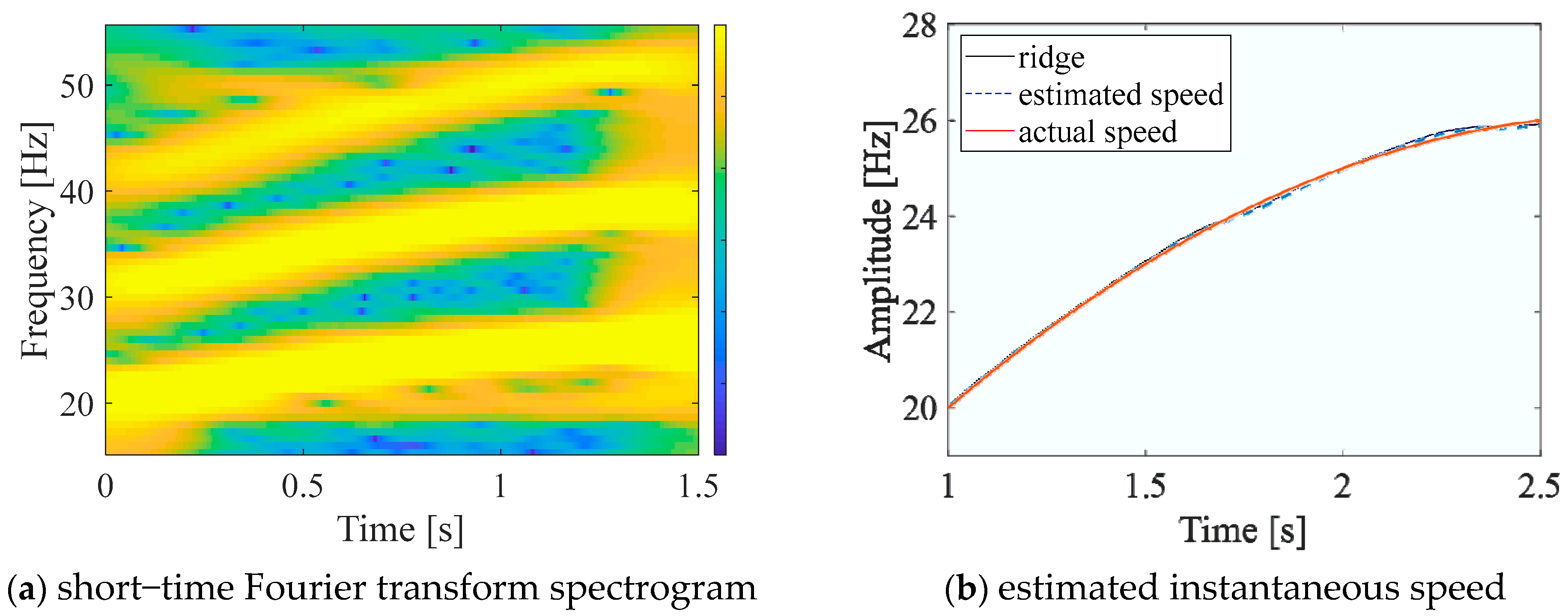
The waveform and Fourier spectrum of the simulated signal are depicted in Figure 4a,b, respectively. Figure 5a illustrates the short–time Fourier transform spectrogram of the simulated signal, revealing the presence of three time–varying harmonic components and two constant frequency components. These frequency components exhibit significant overlap and even crossover in the frequency domain. Additionally, the interference from background noise and limitations in time–frequency resolution further complicate the identification process, making it challenging to determine the frequency structure of the signal. Given the rotational frequency, the signal is resampled in the angular domain according to , as shown in Figure 4c. Subsequently, a Fourier transform is applied to the angular domain resampled signal to obtain the traditional order spectrum, presented in Figure 4d. While three order components can be roughly identified in the figure, their energy is not concentrated at their respective frequency orders but, rather, spreads around them, leading to spectral aliasing between adjacent frequency orders. This is due to the nonstationary nature of the amplitude envelopes in the angular domain, even after equal–angle resampling, resulting in spectral leakage issues in the order spectrum.
To address the above challenges, the proposed method is employed for the identification of frequency components in the signal structure. Initially, the multi–order probabilistic approach is utilized to accurately extract the instantaneous rotational speed from the raw signal, providing a crucial input for subsequent instantaneous frequency calculation. The time–frequency ridge is extracted from the probability density function, and an accurate estimate of the instantaneous rotational speed is obtained through fitting. A comparison of the instantaneous ridge, estimated rotational speed, and actual rotational speed is presented in Figure 5b. The results demonstrate a high degree of agreement between the instantaneous rotational frequency extracted using the multi–order probabilistic approach and the true rotational frequency. This validates the superiority of the proposed method in facilitating effective and efficient estimation of the instantaneous rotational speed without relying on additional rotary encoders or tachometers.
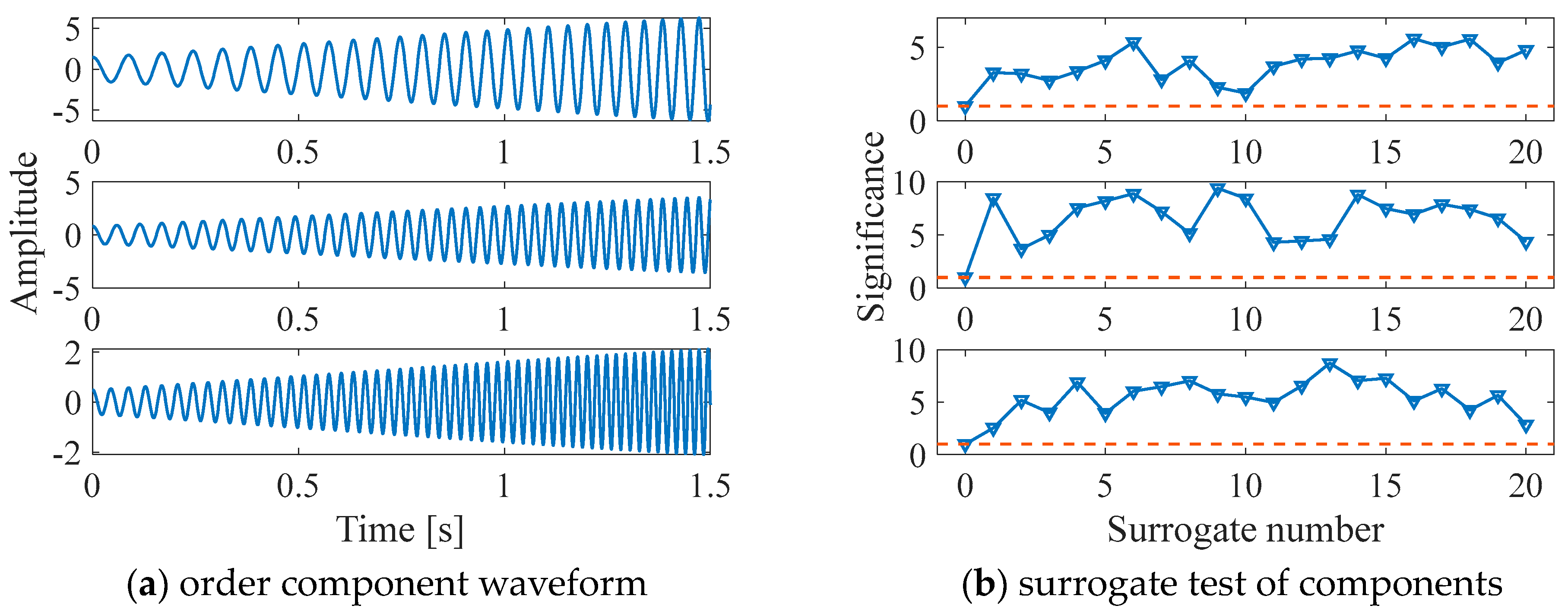
Based on the estimated instantaneous rotational frequency , components can be effectively separated through time–varying filtering. The validity of each separated mono–component is verified through the surrogate test, and the corresponding harmonic orders are determined. Using the obtained rotational frequency , an exhaustive calculation of the instantaneous frequencies for each harmonic order is performed, and they are fully extracted using time–varying filtering. For each component, the generalized demodulation function and inverse demodulation function are denoted as and , respectively, where is set to one–quarter of the sampling frequency. Through iterative applications of generalized demodulation, zero–phase filtering, and inverse generalized demodulation steps, multiple order components are successfully separated. However, not all of these separated components represent true rotational frequency harmonics, as some may be spurious components arising from background noise. To accurately identify the true components and eliminate noise interference, the surrogate test is conducted on the separated components. As shown in Figure 6, among these components, only those with instantaneous frequencies of , , and exhibit lower significance values compared to their surrogate data, indicating that they pass the test and are identified as true components. The other components are recognized as spurious, arising from noise, which aligns perfectly with the actual simulation scenario. Therefore, it can be concluded that the proposed method can adaptively identify and extract true rotational frequency harmonic components while effectively eliminating irrelevant components and background noise interference.
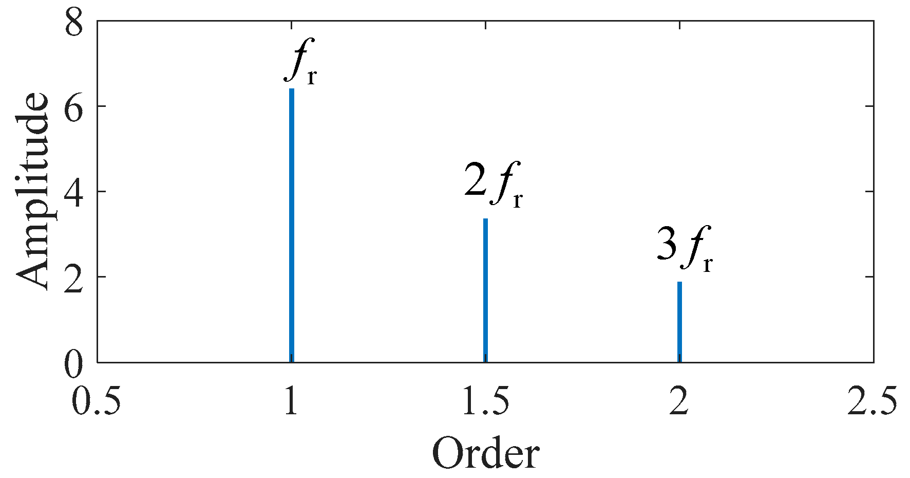
After extracting the rotational frequency harmonic components, the mean values of their amplitude envelopes are further calculated. By assigning the mean amplitude envelope values and corresponding orders to each component, an optimized order spectrum is constructed, as illustrated in Figure 7. Compared to the conventional order spectrum in Figure 4b, the optimized version exhibits a higher concentration of energy at respective frequency orders, boasting superior resolution. It clearly reveals the frequency order structure along with the corresponding amplitude information.
4. Experimental Validations for Rolling Element Bearing Fault Diagnosis
In this section, the proposed method is applied to the amplitude envelopes of bearing vibration signals for the purpose of extracting fault characteristics and facilitating fault diagnosis. This approach serves to validate the effectiveness of the proposed method in accurately identifying and diagnosing faults.
4.1. Experiment Settings
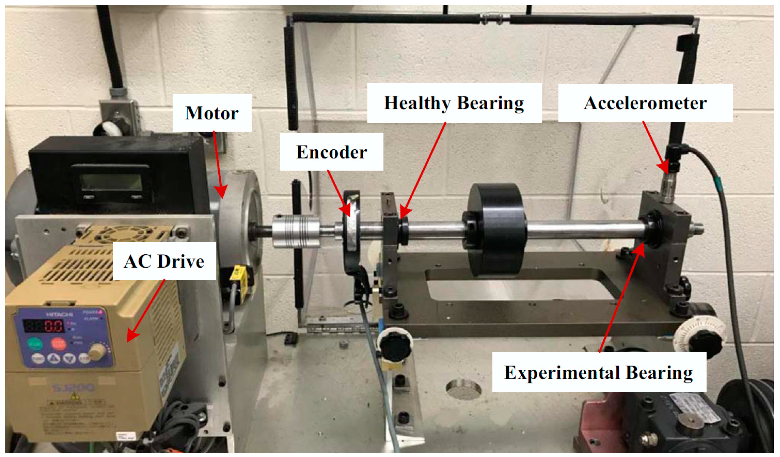
Figure 8 shows a rolling element bearing test rig at the University of Ottawa. Table 1 lists the structural parameters of the bearings. Given the gearbox configuration parameters, the characteristic frequency can be calculated. In the experiment, a defect occurs on outer race of the experimental bearing. An accelerometer is mounted at the top of the experimental bearing, to collect vibration signals at a sampling frequency of 200 kHz for a duration of 7 s.
4.2. Signal Analysis
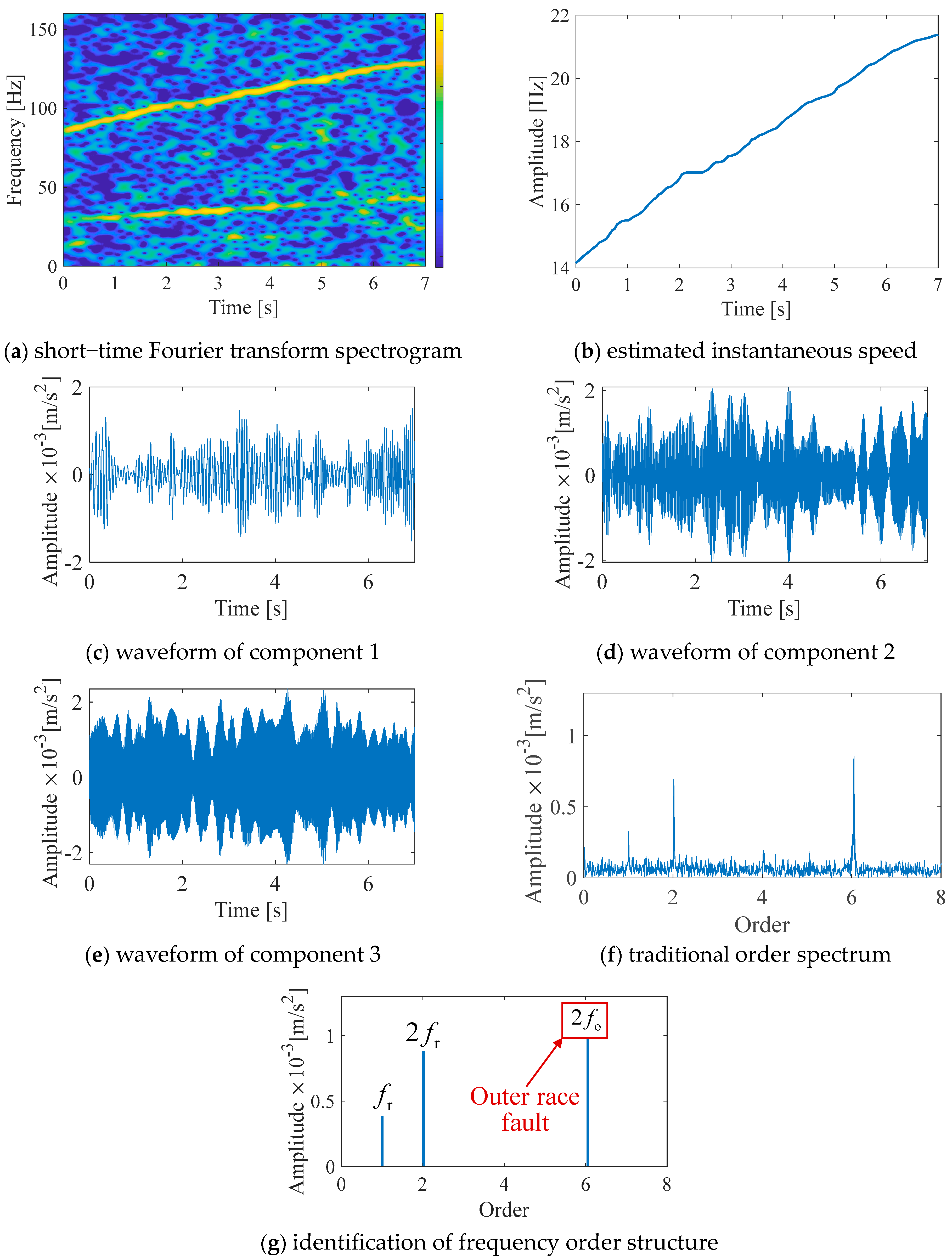
Figure 9a,b present the waveform and Fourier spectrum, respectively. Upon examination of the short–time Fourier transform spectrogram in Figure 10a, the nonstationary nature of the signal, along with noise interference components, becomes evident.
To accurately identify these components, we employed the proposed method. Initially, MOPA was utilized to precisely extract the instantaneous rotational speed information of the main shaft, which is directly connected to the motor, from the intricate raw signal. Subsequently, extraction of the time–frequency ridge lines from the probability density function was conducted, followed by an accurate fitting process to derive the precise instantaneous speed curve, as illustrated in Figure 10b.
Leveraging this instantaneous speed information, we further conducted a comprehensive traversal calculation of the instantaneous frequencies corresponding to various harmonic components. Through an iterative application of sophisticated steps including generalized demodulation, zero–phase filtering, and inverse generalized demodulation, we successfully achieved complete separation of the multi–order components. The surrogate test confirmed the authenticity of the components presented in Figure 10c–e. Subsequently, we calculated the mean amplitude envelopes of these components and combined them with their corresponding order information to construct an optimized order spectrum. Compared to the traditional order spectrogram shown in Figure 10f, the proposed spectrogram depicted in Figure 10g not only reveals the frequency order details with remarkable clarity but also effectively eliminates noise and irrelevant component interference, ensuring purity and accuracy in the analysis results. Within the order features, we distinctly identified the presence of the shaft rotation frequency and its harmonics , along with the outer race fault frequency . This discovery aligns perfectly with the actual fault condition of the bearing outer race, providing a robust foundation for fault diagnosis.
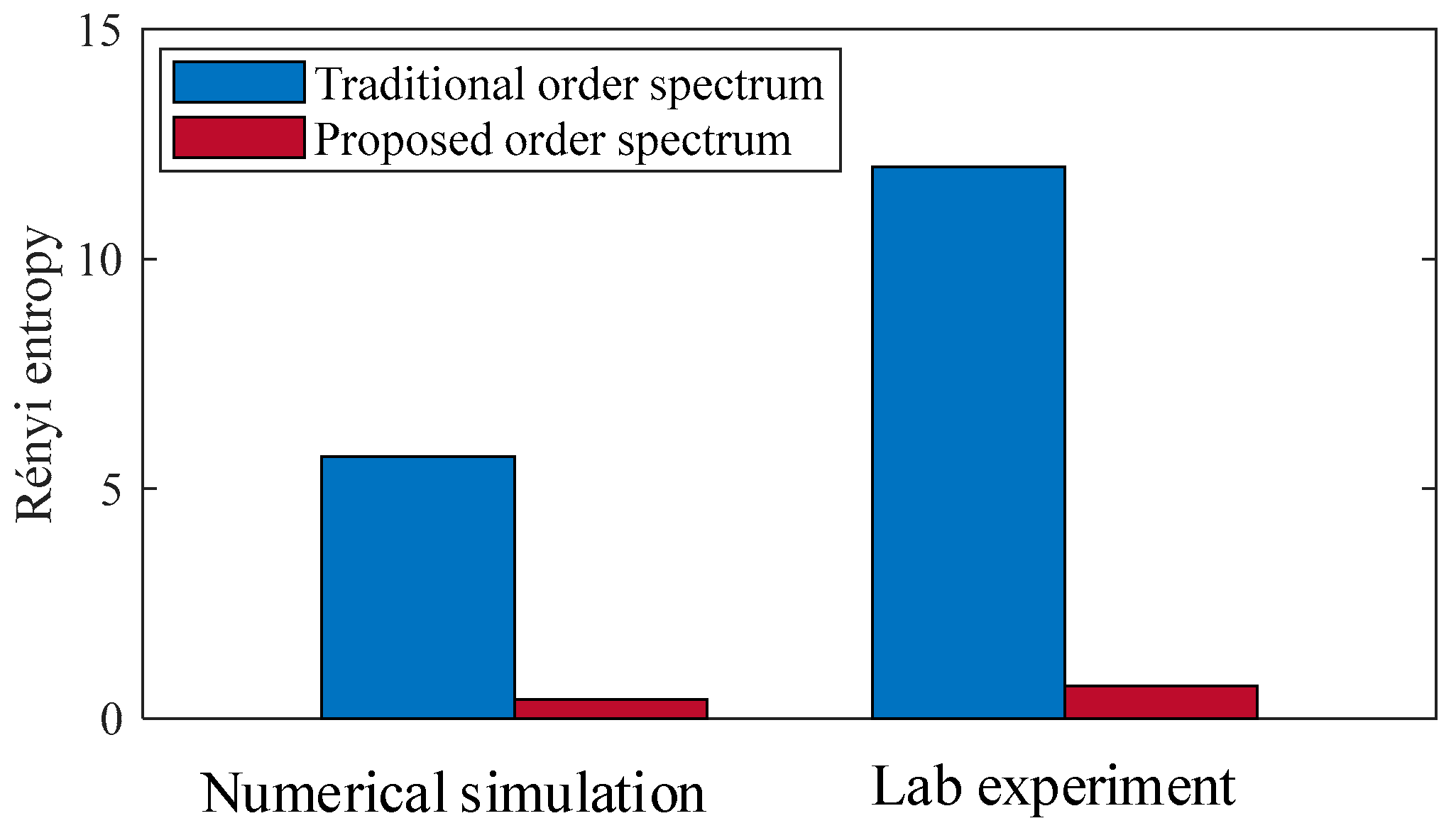
Based on the analysis results of simulation signals and experiment signals, Rényi entropy calculations were performed for both the traditional order spectrum and the proposed order spectrum. The comparison results are presented in Figure 11. Rényi entropy represents the degree of energy concentration in the spectrum, where a smaller entropy value indicates a higher degree of concentration. As shown in the figure, the proposed order spectrum exhibits lower entropy values in both simulation and actual signal applications. This significant result demonstrates the excellent performance of the proposed method in revealing frequency structures, with high resolution, strong readability, and effective energy concentration.
The comparison between the proposed method and the traditional order analysis method is shown in Table 2. The proposed method effectively avoids energy leakage caused by irrelevant components and nonstationarity, and prevents errors introduced by resampling. Compared with the traditional order spectrum, it exhibits more concentrated energy and higher resolution.
5. Conclusions
Order spectrum analysis is widely applied in rotating machinery fault diagnosis under time–varying operating conditions. However, it faces the challenges of inconvenient instantaneous speed measurement, interference from irrelevant components, angular resampling errors, and spectral leakage. To address these issues, a novel method based on adaptive separation of time–varying components and order spectrum construction is proposed. Compared with available methods, no tachometer is required, the interferences from speed–unrelated components are eliminated, and fine spectral resolution is achieved. Results of the numerical simulation prove the correctness of the constructed order spectrum based on adaptive component identification and time–varying amplitude envelope. The outer race fault on a real–world rolling element bearing is successfully diagnosed under time–varying speed conditions, by identifying twice the fault frequency on the constructed order spectrum. In summary, the proposed method is validated to be capable of characterizing time–varying multicomponent signals with high accuracy and little interference, thus supporting rotating machinery fault diagnosis under time–varying speed conditions. However, it should be noted that the proposed method has its limitations. The process involved is relatively complex, requiring multiple steps and computations. Additionally, the method demands a significant amount of computational power, which may pose challenges in real–time applications or when dealing with large datasets. Despite these limitations, the method still offers valuable insights into rotating machinery fault diagnosis under time–varying speed conditions.
Author Contributions
Conceptualization, X.Y.; methodology, X.C.; software, M.D.; validation, Y.Y.; formal analysis, M.D.; investigation, Y.Y.; resources, Z.F.; data curation, Z.F.; writing—original draft preparation, X.Y.; writing—review and editing, X.C.; visualization, Z.F. All authors have read and agreed to the published version of the manuscript.
Funding
This research received no external funding.
Data Availability Statement
All data generated or analyzed during the study are included in this published article.
Conflicts of Interest
The authors declare no conflict of interest.
References
- Cheng, Y.; Chen, B.Y.; Zhang, W.H. Adaptive Multipoint Optimal Minimum Entropy Deconvolution Adjusted and Application to Fault Diagnosis of Rolling Element Bearings. IEEE Sens. J. 2019, 19, 12153–12164. [Google Scholar] [CrossRef]
- Rafiq, H.J.; Rashed, G.I.; Shafik, M.B. Application of multivariate signal analysis in vibration–based condition monitoring of wind turbine gearbox. Int. Trans. Electr. Energy Syst. 2021, 31, e12762. [Google Scholar] [CrossRef]
- Qin, A.S.; Hu, Q.; Zhang, Q.H.; Lv, Y.R.; Sun, G.X. Application of sensitive dimensionless parameters and PSO–SVM for fault classification in rotating machinery. Assem. Autom. 2019, 40, 175–187. [Google Scholar] [CrossRef]
- Xu, X.L.; Liu, X.L. Fault Diagnosis Method for Wind Turbine Gearbox Based on Image Characteristics Extraction and Actual Value Negative Selection Algorithm. Int. J. Pattern. Recognit. Artif. Intell. 2020, 34, 2054034. [Google Scholar] [CrossRef]
- Peng, G.; Xu, D.; Zhou, J.; Yang, Q.; Shen, W. A novel curve pattern recognition framework for hot–rolling slab camber. IEEE Trans. Ind. Inform. 2022, 19, 1270–1278. [Google Scholar] [CrossRef]
- Peng, G.; Cheng, Y.; Zhang, Y.; Shao, J.; Wang, H.; Shen, W. Industrial big data–driven mechanical performance prediction for hot–rolling steel using lower upper bound estimation method. J. Manuf. Syst. 2022, 65, 104–114. [Google Scholar] [CrossRef]
- Fyfe, K.R.; Munck, E.D.S. Analysis of Computed Order Tracking. Mech. Syst. Signal Process. 1997, 11, 187–205. [Google Scholar] [CrossRef]
- Lu, S.; Yan, R.; Liu, Y.; Wang, Q. Tacholess Speed Estimation in Order Tracking: A Review With Application to Rotating Machine Fault Diagnosis. IEEE Trans. Instrum. Meas. 2019, 68, 2315–2332. [Google Scholar] [CrossRef]
- Xu, L.; Ding, K.; He, G.; Li, W.; Li, J. A novel tacholess order tracking method for gearbox vibration signal based on extremums search of gear mesh harmonic. Mech. Syst. Signal Process. 2023, 189, 110070. [Google Scholar] [CrossRef]
- Potter, R.; Gribler, M. Computed Order Tracking Obsoletes Older Methods. In Proceedings of the SAE Noise and Vibration Conference, West Palm Beach, FL, USA, 8–10 February 1989; pp. 63–67. [Google Scholar]
- Li, B.; Zhang, X. A New Strategy of Instantaneous Angular Speed Extraction and Its Application to Multistage Gearbox Fault Diagnosis. J. Sound. Vib. 2017, 396, 340–355. [Google Scholar] [CrossRef]
- Rémond, D.; Antoni, J.; Randall, R. Editorial for the special issue on Instantaneous Angular Speed (IAS) processing and angular applications. Mech. Syst. Signal Process. 2014, 44, 1–4. [Google Scholar] [CrossRef]
- Peeters, C.; Leclère, Q.; Antoni, J.; Lindahl, P.; Donnal, J.; Leeb, S.; Helsen, J. Review and comparison of tacholess instantaneous speed estimation methods on experimental vibration data. Mech. Syst. Signal Process. 2019, 129, 407–436. [Google Scholar] [CrossRef]
- Zhao, M.; Lin, J.; Xu, X.; Lei, Y. Tacholess envelope order analysis and its application to fault detection of rolling element bearings with varying speeds. Sensors 2013, 13, 10856–10875. [Google Scholar] [CrossRef]
- Hu, Y.; Cui, F.; Tu, X.; Li, F. Bayesian estimation of instantaneous speed for rotating machinery fault diagnosis. IEEE Trans. Ind. Electron. 2021, 68, 8842–8852. [Google Scholar] [CrossRef]
- Gu, L.; Tian, Q.; Ma, Z. Extraction of the instantaneous speed fluctuation based on normal time–frequency transform for hydraulic system. Proc. Inst. Mech. Engineers. Part C J. Mech. Eng. Sci. 2020, 234, 1196–1211. [Google Scholar] [CrossRef]
- Leclère, Q.; André, H.; Antoni, J. A multi–order probabilistic approach for instantaneous angular speed tracking debriefing of the CMMNO’ 14 diagnosis contest. Mech. Syst. Signal Process. 2016, 81, 375–386. [Google Scholar] [CrossRef]
- Peeters, C.; Leclere, Q.; Antoni, J.; Guillaume, P.; Helsen, J. Vibration–based angular speed estimation for multi–stage wind turbine gearboxes. J. Phys. Conf. Ser. 2017, 842, 012053. [Google Scholar] [CrossRef]
- Schmidt, S.; Heyns, P.S.; De Villiers, J.P. A tacholess order tracking methodology based on a probabilistic approach to incorporate angular acceleration information into the maxima tracking process. Mech. Syst. Signal Process. 2018, 100, 630–646. [Google Scholar] [CrossRef]
- Gryllias, K.; Andre, H.; Leclere, Q.; Antoni, J. Condition monitoring of rotating machinery under varying operating conditions based on cyclononstationary indicators and a multi–order probabilistic approach for instantaneous angular speed tracking. IFAC–PapersOnLine 2017, 50, 4708–4713. [Google Scholar]
- Wang, K.; Heyns, P.S. The combined use of order tracking techniques for enhanced fourier analysis of order components. Mech. Syst. Signal Process. 2011, 25, 803–811. [Google Scholar] [CrossRef]
- Wang, K.; Guo, D.; Heyns, P.S. The application of order tracking for vibration analysis of a varying speed rotor with a propagating transverse crack. Eng. Fail. Anal. 2012, 21, 91–101. [Google Scholar] [CrossRef]
- Zhao, M.; Lin, J.; Wang, X.; Lei, Y.; Cao, J. A tacho–less order tracking technique for large speed variations. Mech. Syst. Signal Process. 2013, 40, 76–90. [Google Scholar] [CrossRef]
- Coats, M.D.; Randall, R.B. Single and multi–stage phase demodulation based order–tracking. Mech. Syst. Signal Process. 2014, 44, 86–117. [Google Scholar] [CrossRef]
- Blough, J.R.; Brown, D.L.; Vold, H. The time variant discrete Fourier transform as an order tracking method. SAE Trans. 1997, 106, 3037–3045. [Google Scholar]
- Borghesani, P.; Pennacchi, P.; Chatterton, S.; Ricci, R. The velocity synchronous discrete Fourier transform for order tracking in the field of rotating machinery. Mech. Syst. Signal Process. 2014, 44, 118–133. [Google Scholar] [CrossRef]
- Xu, S.; Zhang, Y.; Pham, D. Antileakage Fourier transform for seismic data regularization. Geophysics 2005, 70, V87–V95. [Google Scholar] [CrossRef]
- Xu, S.; Zhang, Y.; Lambaré, G. Antileakage Fourier transform for seismic data regularization in higher dimensions. Geophysics 2010, 75, WB113–WB120. [Google Scholar] [CrossRef]
- Schonewille, M.; Klaedtke, A.; Vigner, A. Anti–alias anti–leakage Fourier transform. In Proceedings of the SEG International Exposition and Annual Meeting, Houston, TX, USA, 25–30 October 2009; pp. 3249–3253. [Google Scholar]
- Zhang, F.; Geng, Z.; Yuan, W. The algorithm of interpolating windowed FFT for harmonic analysis of electric power system. IEEE Trans. Power Deliv. 2001, 16, 160–164. [Google Scholar] [CrossRef]
- Schreiber, T.; Schmitz, A. Surrogate time series. Phys. D Nonlinear Phenom. 2000, 142, 346–382. [Google Scholar] [CrossRef]
- Theiler, J.; Eubank, S.; Longtin, A.; Galdrikian, B.; Farmer, J.D. Testing for nonlinearity in time series: The method of surrogate data. Phys. D Nonlinear Phenom. 1992, 58, 77–94. [Google Scholar] [CrossRef]
Figure 1.
Schematic diagram of instantaneous rotational speed estimation.

Figure 2.
Schematic diagram of time–varying filtering.

Figure 3.
Flowchart of the proposed adaptive high–resolution order spectrum.
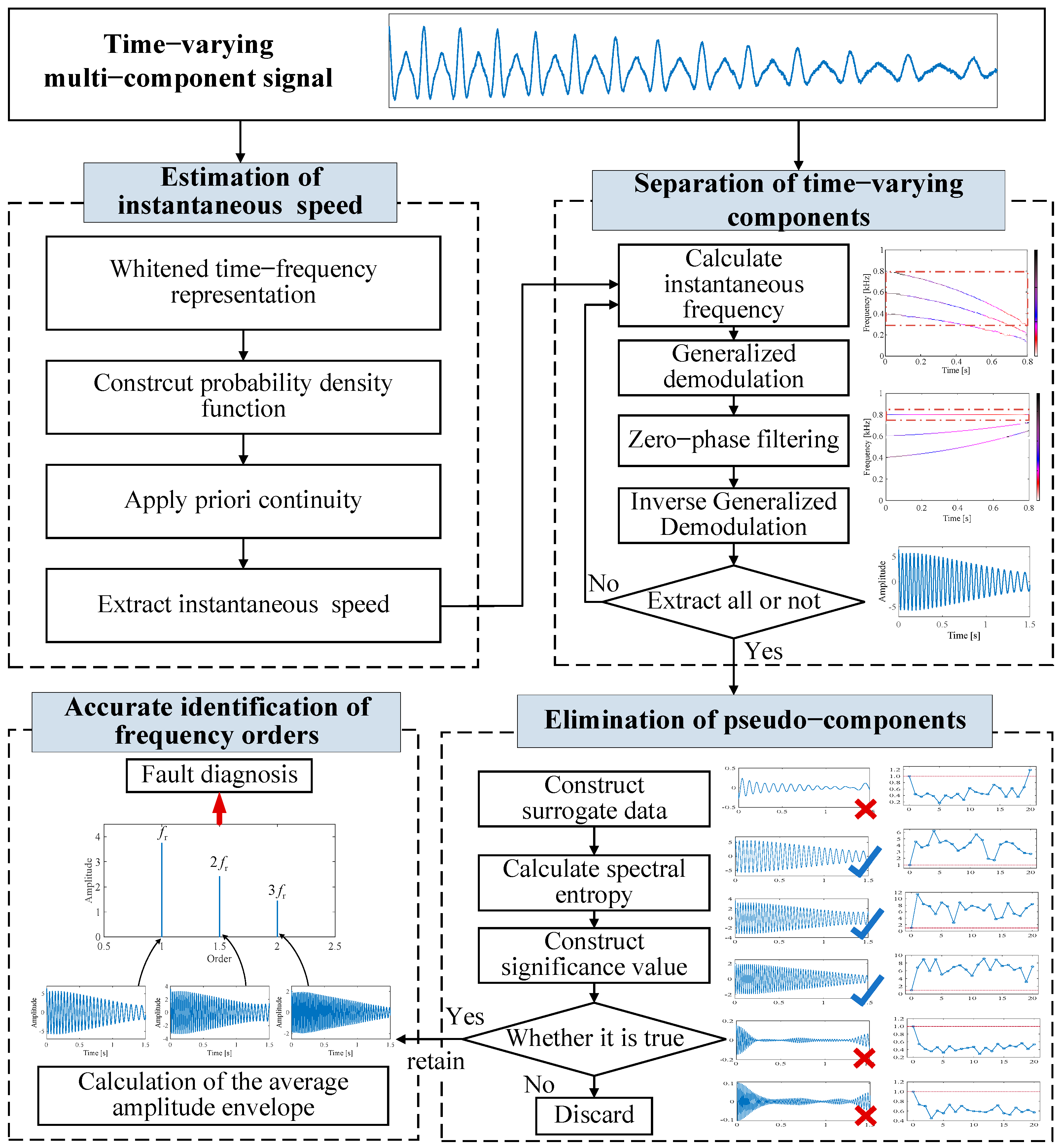
Figure 4.
Traditional order analysis results of multi–harmonic component simulation signal.
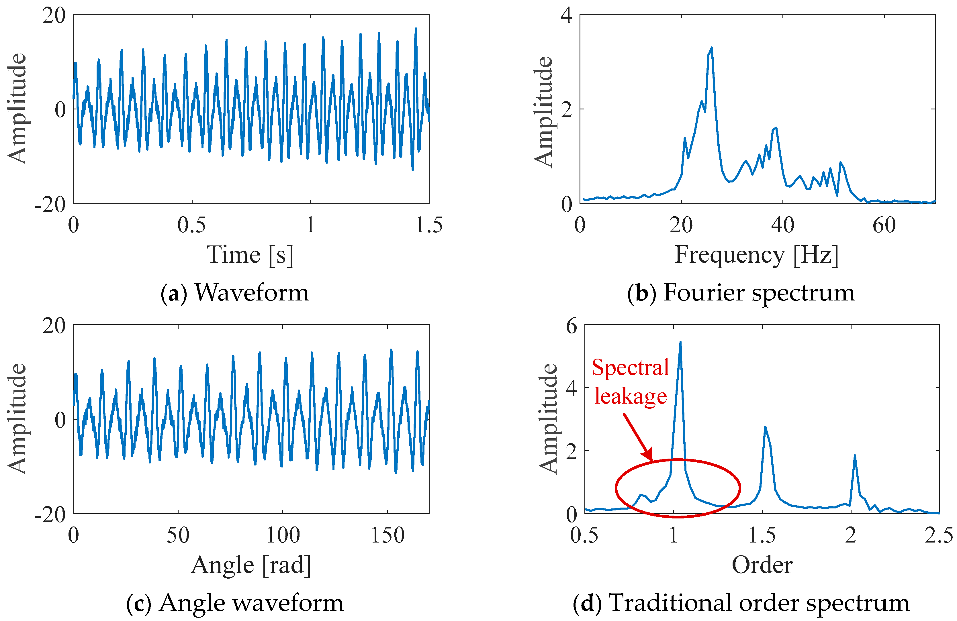
Figure 5.
Accurate estimation of instantaneous speed.

Figure 6.
Extraction of time–varying component.

Figure 7.
Accurate identification of frequency order structure.

Figure 8.
Rolling element bearing test rig configuration.

Figure 9.
Outer race fault signal of rolling element bearing.
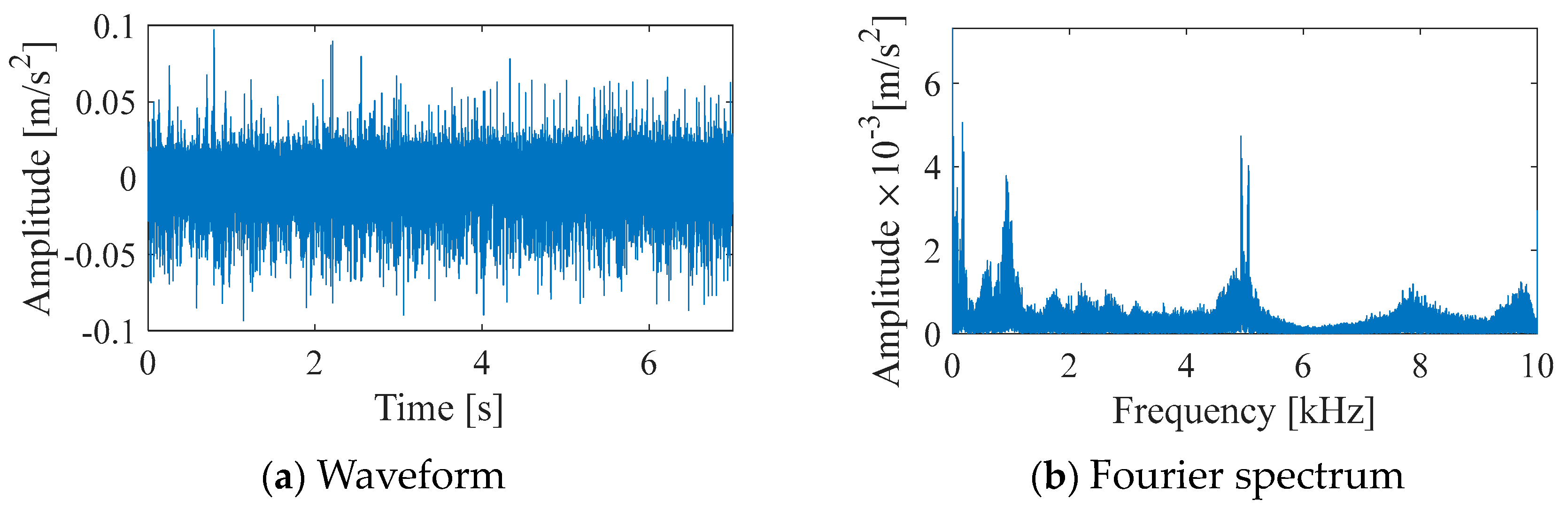
Figure 10.
Fault diagnosis of rolling element bearing signal.

Figure 11.
Comparison of Rényi entropy.


Table 1.
Bearing configuration.
| Bearing Parameters | Characteristic Frequency | |||
|---|---|---|---|---|
| Pitch Diameter | Ball Diameter | Number of Balls | BPFI | BPFO |
| 38.52 mm | 7.94 mm | 9 | 5.43fr | 3.57fr |
Table 2.
Comparison of our study with existing work.
| Traditional Order Spectrum | Proposed Order Spectrum | |
|---|---|---|
| Is rotational speed data required? | Yes | No |
| Does energy leakage exist due to irrelevant components? | Yes | No |
| Does energy leakage exist due to nonstationarity? | Yes | No |
| Does error exist due to resampling? | Yes | No |
| Spectral energy concentration | Low | High |
Disclaimer/Publisher’s Note: The statements, opinions and data contained in all publications are solely those of the individual author(s) and contributor(s) and not of MDPI and/or the editor(s). MDPI and/or the editor(s) disclaim responsibility for any injury to people or property resulting from any ideas, methods, instructions or products referred to in the content. |
© 2024 by the authors. Licensee MDPI, Basel, Switzerland. This article is an open access article distributed under the terms and conditions of the Creative Commons Attribution (CC BY) license (https://creativecommons.org/licenses/by/4.0/).
Share and Cite
MDPI and ACS Style
Yu, X.; Chen, X.; Du, M.; Yang, Y.; Feng, Z. Rotating Machinery Fault Diagnosis under Time–Varying Speed Conditions Based on Adaptive Identification of Order Structure. Processes 2024, 12, 752. https://doi.org/10.3390/pr12040752
AMA Style
Yu X, Chen X, Du M, Yang Y, Feng Z. Rotating Machinery Fault Diagnosis under Time–Varying Speed Conditions Based on Adaptive Identification of Order Structure. Processes. 2024; 12(4):752. https://doi.org/10.3390/pr12040752
Chicago/Turabian StyleYu, Xinnan, Xiaowang Chen, Minggang Du, Yang Yang, and Zhipeng Feng. 2024. "Rotating Machinery Fault Diagnosis under Time–Varying Speed Conditions Based on Adaptive Identification of Order Structure" Processes 12, no. 4: 752. https://doi.org/10.3390/pr12040752
Note that from the first issue of 2016, this journal uses article numbers instead of page numbers. See further details here.