Abstract
In low-voltage distribution networks, distributed energy storage systems (DESSs) are widely used to manage load uncertainty and voltage stability. Accurate modeling and estimation of voltage fluctuations are crucial to informed DESS dispatch decisions. However, existing parametric probabilistic approaches have limitations in handling complex uncertainties, since they always rely on predefined distributions and complex inference processes. To address this, we integrate the patch time series Transformer model with the non-parametric Huberized composite quantile regression method to reliably predict voltage fluctuation without distribution assumptions. Comparative simulations on the IEEE 33-bus distribution network show that the proposed model reduces the DESS dispatch cost by 6.23% compared to state-of-the-art parametric models.
1. Introduction
Effective voltage management is essential to ensure the safe and stable operation of low-voltage distribution networks [1,2]. However, the random nature of electrical loads presents a significant challenge in maintaining the bus voltage within the nominal range [3]. These uncertainties may result in voltage fluctuations or exceedances, thereby jeopardizing the stability and reliability of the power grid [4]. In recent decades, the distributed energy storage system (DESS) has emerged as a vital solution to manage this challenge and maintain voltage safety [5,6].
The accurate estimation of voltage fluctuation caused by the stochastic characteristics of loads [7] enables the optimal dispatch of DESSs. Existing techniques for handling uncertainties in distribution networks primarily include scenario-based stochastic programming [8,9], robust optimization [10,11], chance-constrained programming [12,13], etc. Among these, the chance-constrained programming approach is an effective approach that directly incorporates uncertainties into the optimization model by defining constraints that must be satisfied with a certain probability [14].
There are existing studies that investigate the formulations and solving methods for the chance-constrained economic dispatch (CCED) problem. Ref. [15] introduces a new probabilistic distribution model, called versatile distribution, to represent prediction errors in wind power. This probabilistic distribution model is incorporated into the CCED problem that includes wind power, with the aim of reducing the non-linearity and complexity of the problem. Ref. [16] also utilizes the versatile distribution to model the stochastic output of wind turbines, thus transforming the probabilistic constraints of wind power in the proposed decentralized CCED model into deterministic constraints. Although the fitting accuracy of the versatile distribution has been shown to outperform the Gussian and Bata distributions, the parametric probabilistic forecasting method may face limitations when dealing with complex uncertainties [14]. Therefore, some studies have begun exploring non-parametric probabilistic forecasting methods to better capture the uncertainties of renewable energy or electricity load. Ref. [17] combines extreme learning machines and quantile regression to efficiently produce non-parametric probability forecasts for wind power generation. Ref. [18] formulates a CCED model for DESS planning in active distribution networks, utilizing empirical probability density functions without parametric assumptions and a numerical convolution method to deal with uncertainties of various distributed energy resources (DERs). These studies validate that non-parametric probabilistic forecasting methods can accurately estimate various quantiles of random variables in the CCED problem without the need for any prior knowledge, statistical inference, or the assumption of specific probability distributions. This enables a more accurate and efficient conversion of the uncertain CCED problem into a linear programming problem.
Furthermore, with the applicability and extensibility of deep learning methods continuously verified [19,20,21], their capabilities in time series forecasting have received widespread attention [22,23,24,25]. Recently, the channel-independent patch time series Transformer (PatchTST) model has been proven to exhibit exceptional performance in time series prediction [26]. Its channel-independent processing, patching processing, and the Transformer architecture together enhance the model’s deep understanding of both global trends and granularity in time-series data. Therefore, it is highly suitable to predict voltage fluctuations in distribution networks affected by random loads.
In this paper, we integrate a non-parametric probabilistic forecasting approach, Huberized Composite Quantile Regression (HuberCQR), into the Transformer-based PatchTST model, to address the uncertainty of random loads in the DESS CCED problem. HuberCQR is an effective technique that combines the robustness of Huber loss [27,28] with the flexibility of composite quantile regression (CQR) [29], enabling the model to generate accurate probabilistic forecasts even in the presence of noisy or outlier data. By integrating CQR into the PatchTST framework, we aim to leverage the Transformer’s ability to capture complex temporal relationships while enhancing its prediction accuracy and efficiency across different quantiles. This integration allows for more reliable and robust forecasting of non-stationary voltage uncertainties, thereby facilitating more efficient and effective decision-making in the DESS CCED problem.
Overall, the contributions of this paper can be concluded as follows: (1) This paper leverages the non-parametric HuberCQR method to estimate composite quantiles of the uncertain voltage fluctuation caused by random loads, which is vital for transforming the original DESS CCED problem into linear form without complex mathematical derivations and predefined probabilistic assumptions. (2) The Transformer-based PatchTST forecasting framework integrated with the HuberCQR loss function is utilized to efficiently learn the uncertainties of bus voltage fluctuations. (3) The Transformer-based non-parametric probabilistic prediction framework demonstrates superior performance in providing accurate quantification of the voltage fluctuation range, which facilitates an effective trade-off between the DESS dispatch cost and the voltage violation risk.
The remainder of this paper is organized as follows. The problem formulation of the DESS CCED for voltage management in the distribution network is introduced in Section 2. Section 3 presents the Transformer-based PatchTST forecasting framework integrated with the HuberCQR loss function for composite quantile predictions of voltage fluctuation. In Section 4, comprehensive case studies are conducted to verify the effective and economical dispatch of DESS based on the proposed method. Finally, Section 5 concludes the paper.
2. Problem Formulation
In this section, we formulate a day-ahead DESS CCED problem for voltage management in a distribution network considering load uncertainty. Then we demonstrate how to transform chance constraints into deterministic constraints by introducing the cumulative distribution function (CDF) of a random variable and its inverse function: quantile function.
2.1. Linear DistFlow Model
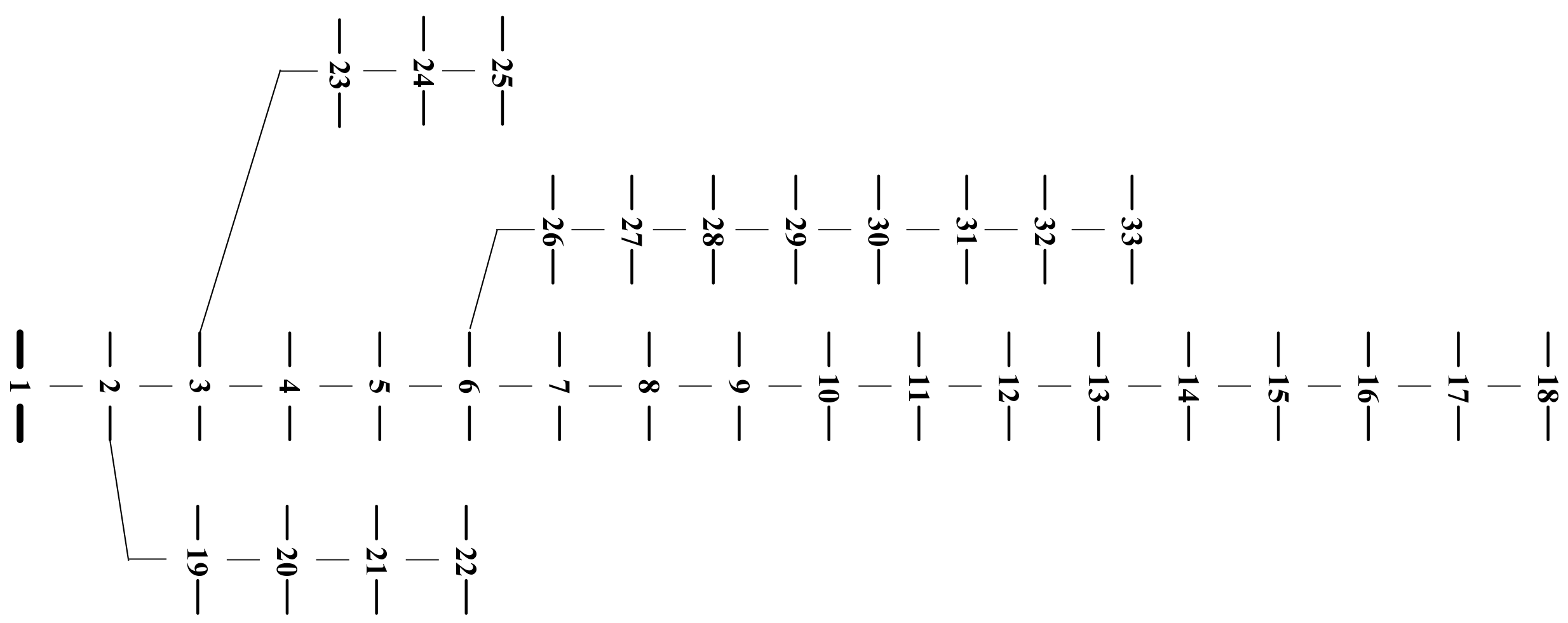
Consider a radial distribution network denoted by , where represents the distribution network buses and represents the distribution lines. Let represent the branch on the direct path from bus i to the reference bus, with denoting the non-reference bus. Define the set of descendants of bus m as , and each branch between two buses as . Take the IEEE 33-bus distribution network (shown in Figure 1) as an illustrative case, where bus #1 is the reference bus with a voltage magnitude of 1 p.u. The set includes direct branches connecting bus #25 to the reference bus, i.e., , and refers to the descendants of bus #6, i.e., .

Figure 1.
IEEE 33-bus radial distribution network [30].
In this paper, we adopt the Linear DistFlow model to describe the power flow in the distribution network [31,32], and assume a common scenario where the DESS only offers active power support [18]:
where represents the bus voltage squared, calculated based on the line resistance and reactance , considering the active and reactive power flows and . The active power flows and are determined by adding the active power consumption of DESSs and random loads on all descendants of the bus m, while reactive power flow is calculated as the sum of net reactive power consumption . This linear power flow model illustrates how the spatial distribution and electrical power of DESSs and random loads influence the bus voltage.
2.2. Objective and Constraints
This section introduces the objectives and constraints of the DESS CCED problem and presents the deterministic conversion of the chance constraints.
2.2.1. Objective
The objective of the DESS CCED problem in this paper is to minimize the total operational cost of all DESSs in the distribution network [33] as formulated in Equation (4):
where is the set of all DESSs in the distribution network, T is the entire dispatch horizon, is the cost per unit of charging and discharging of a DESS ($/MWh), is the charging and discharging efficiency (%), and are the charging and discharging power of DESS i at time t (MW), and is the dispatch time interval.
This formulation reflects the wear cost from battery degradation due to the charging/discharging operation. Under a reasonable depth of discharge, the overall capacity for charging/discharging of a DESS remains at a certain level. Therefore, the wear cost can be considered to be nearly proportional to the charging/discharging energy. Moreover, the term considers the energy loss during the charging and discharging process due to efficiency.
2.2.2. Constraints
The DESS CCED problem should be subject to the following constraints:
where and represent the charging and discharging states of DESS i at time t, with a value of 1 indicating charging/discharging and 0 otherwise; and mean the maximum allowable charging/discharging power of DESS; SOC is the state of charge of the battery, indicating the ratio of the remaining capacity to the total capacity; and signify the minimum/maximum allowed SOC lower limits of DESS i; represents the DESS capacity; is bus voltage at time t calculated by the Equation (1); and represent the lower/upper voltage thresholds of bus i; and symbolizes the allowed violation probability of the voltage constraint.
Equations (5)–(9) define the operational constraints of the DESS unit. More specifically, Equations (5) and (6) give the limits of the DESS charging and discharging power. Equation (7) indicates that DESS cannot be simultaneously in charging and discharging states. Equations (8) and (9) describe the energy balance and depth of discharge (DOD) limit of DESS. Equations (10) and (11) assume that the probability of bus voltage violation remains below a certain level, which is vital for the safe operation of the power system.
2.2.3. Deterministic Conversion of Chance Constraints
To solve the formulated DESS CCED model (4)–(11), the chance constraints (10) and (11) need to be transformed into deterministic constraints. Then, the optimal solution of the formulated model can be obtained directly by applying professional solvers to the resulting mixed-integer linear programming (MILP) problem. Next, the conversion of chance constraints into deterministic linear constraints will be explained.
To begin with, we substitute Equations (1)–(3) into (10) and obtain:
Then, a new random variable is defined, which indicates the voltage drop caused by random loads compared with the reference voltage (1 p.u.) at the reference bus:
Thereafter, Equation (12) can be expressed as Equation (14) by substituting Equation (13). Equation (15) takes the complement of Equation (14). Next, Equation (16) substitutes the CDF definition for the probability term in Equation (15), which reflects the probability that the random variable is less than or equal to a certain value. Finally, Equation (17) incorporates the inverse CDF term, , resulting in an equivalent expression of the original chance constraint but now in a deterministic form:
A similar transformation can be applied to Equation (11), resulting in:
In Equations (17) and (18), and can be interpreted as the quantiles of at level and , according to the inverse relationship between CDF and the quantile function. For simplicity of notation, we denote and by and , respectively. In other words, the voltage violation probability is also the probability level that defines . Thus, the key to transforming the DESS CCED model into a directly solvable MILP problem is being able to accurately obtain quantiles of .
However, the probability distributions of bus voltage fluctuations are often complex and unknown, which is due to the network topology and random loads. In addition, analytical expressions of the quantile function may not be obtainable even though the distribution is known. Therefore, technique is needed to accurately predict the values of the voltage fluctuation probability distribution at composite quantiles without relying on the assumptions of underlying probability distribution and complex numerical derivation.
In Section 3, we will introduce a learning-driven prediction model, which leverages the strengths of the improved Transformer model for time series forecasting and the robust CQR method for multi-quantile output. The proposed prediction model can efficiently capture the bus voltage fluctuation patterns affected by temporal random loads.
3. Transformed-Based Non-Parametric Probabilistic Prediction Model
In this section, we introduce the PatchTST prediction model combined with the HuberCQR method for the estimation of .
PatchTST is a deep learning model that excels at capturing complex temporal patterns in time series data. In our problem, we use the PatchTST model to learn the patterns of voltage fluctuations at each non-reference bus caused by random loads. CQR is a non-parametric statistical method that can simultaneously estimate composite quantiles of a variable. It extends traditional quantile regression, which estimates a single quantile at a time. HuberCQR is a robust improvement over the CQR method, where it introduces Huber loss to make CQR predictions less sensitive to outliers.
Specifically, in our framework, we utilize the HuberCQR method to define a loss function, which measures the difference between real data and predicted composite quantiles. The training process of the PatchTST model aims to minimize the average of this HuberCQR loss function over the entire training period. Overall, the integration of the PatchTST model and HuberCQR loss function forms a powerful framework that can capture temporal fluctuations of voltages at different buses in the distribution network, and generate composite predictions at specified probability levels.
3.1. PatchTST Prediction Model
This section introduces the framework of the PatchTST prediction model combined with the HuberCQR loss function, and then outlines its key components.
3.1.1. PatchTST Framework
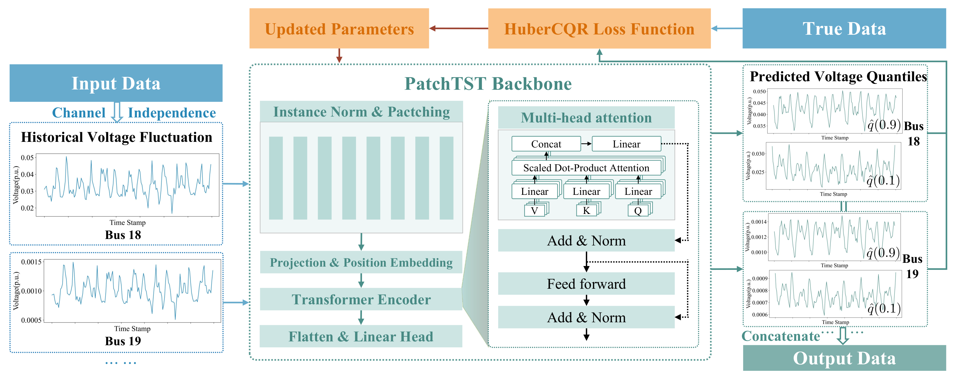
The framework of the PatchTST prediction model is given in Figure 2. The model’s inputs are the collection of historical data of , namely, the voltage drop fluctuations at each non-reference bus, calculated by Equation (13). The outputs are the predictions of at different quantile levels, i.e., .

Figure 2.
The framework of PatchTST.
Initially, PatchTST divides the input multi-bus voltage time series into separate channels. Then, the independent multi-bus voltage time series in each channel is normalized to ensure consistency across different scales. Following normalization, each time series is segmented into patches. After that, the projection and position embedding step projects each patch into a higher-dimensional space and integrates position embedding, to preserve the sequential context of the original time series. The Transformer Encoder, which is the essence of the classic Transformer frameworks, then analyzes patches and understands both overarching trends and fine-grained temporal dynamics in the voltage data. Further, the Flatten and Linear Head step combines the output of the Transformer Encoder by flattening it and using a linear transformation to produce accurate voltage predictions at various quantiles. Once the PatchTST backbone processes the data, the predicted voltage drops at different quantiles, and are compared against actual values using the HuberCQR loss function. By minimizing the HuberCQR loss, the model’s parameters are updated, resulting in a trained PatchTST model. Finally, the well-trained PatchTST model outputs a concatenation of composite quantiles on different buses.
3.1.2. Core Components of PatchTST Backbone
PatchTST enhances prediction capabilities, mainly benefiting from three core components: channel independence process, patching process, and the multi-head attention mechanism of the Transformer backbone.
Channel Independence for Precision Analysis: Channel independence refers to the treatment of separating multivariate time series into individual channels which share the same embedding and Transformer weights. In the context of our problem, PatchTST separates the voltage fluctuation time series for each bus () into distinct channels. This segregation allows for the generation of customized attention maps for each bus voltage, ensuring the accuracy of voltage predictions. The channel-independence model has several advantages over the channel-mixing model: (1) reducing computational complexity and improving processing speed, as the model can process each channel in parallel and a faster learning convergence rate can be achieved; (2) reducing risk of over-fitting, due to the smaller number of parameters for modeling complex interactions between different channels; and (3) increasing robustness to noise by preventing its propagation across mixed channels.
Efficient Data Segmentation with Patching: PatchTST employs a patching technique to effectively manage high-dimensional time series data. This technique divides a time series into N patches of length P, denoted as , achieving a reduction in time and space complexity by a factor of stride: . This technique not only captures the local information within each subsequence but also eases the computational and storage pressure when processing the entire series, enhancing model performance and efficiency.
Comprehensive Insight with Multi-Head Attention Mechanism: The multi-head attention mechanism in PatchTST is vital for analyzing complex dependencies in the input patches on various time scales. Specifically, the multi-head attention mechanism operates through the following steps:
- 1.
- Input Transformation: This step transforms each patch as a whole to capture different aspects of the data. For each attention head i, the entire patches represented by original queries (Q), keys (K), and values (V) are transformed by multiplying the respective weight matrices , , and . This transformation is expressed by Equation (19):Here, the transformation is applied at the patch level, treating each patch as an entity to grasp its unique characteristics and relationships with other patches.
- 2.
- Scaled Dot-Product Attention: This step assesses the relevance of each patch in relation to the others by calculating the similarity between queries and keys at the patch level. For each head i, the similarity between transformed queries and keys is determined by dot products and scaling. The similarity scores for each head are then converted into a probability distribution using the softmax function. A weighted summation is performed on the transformed values based on this distribution as shown in Equation (20):This process enables the model to prioritize patches based on their significance in predicting outcomes, emphasizing the importance of understanding interactions at the patch level.
- 3.
- Output Merging: By integrating insights from all heads, this step provides a comprehensive analysis that improves prediction accuracy through various temporal perspectives. The concatenated outputs of all heads are merged via an additional linear transformation as illustrated by Equation (21):where is the weight matrix designed to combine the insights from individual patches.
3.2. HuberCQR Loss Function
As illustrated in Section 3.1.1, the loss function is the key to training the PatchTST model. In Ref. [26], where the PatchTST method was first introduced, the loss function of mean squared error was used to measure the discrepancy between the predicted values and actual values, but this design was only suitable for point predictions. In our case, we aim to obtain composite probabilistic predictions. In addition, it is significant to ensure the accuracy of the prediction throughout the distribution range for quantile predictions. Thus, we integrate the Huber loss function to provide a more reliable error metric that is less sensitive to extreme deviations. Next, we will provide a detailed description of the HuberCQR loss function.
First, the classic formula for quantile regression is [34]:
where t is the total training epochs, is the quantile level of interest, is the true data, is the predicted quantile value, and is the quantile loss function, defined as:
where , which is the difference between the actual value and the predicted quantile value . Note that the quantile loss function applies penalties to residuals in a way that captures the asymmetry inherent in quantile estimation, giving different importance to underestimations and overestimations relative to the target quantile level.
However, in the classic quantile regression formula, the objective is to find the model parameters that minimize the overall loss. This allows the prediction model to estimate the single quantile of interest. CQR extends this original loss function by simultaneously estimating composite quantiles of interest. The loss function of CQR can be written as follows, which minimizes the average quantile loss [29]:
where measures the quantile loss for the -th quantile , and represents the optimal parameters set of prediction model.
Although the CQR loss function addresses the concern of estimating composite quantiles simultaneously, it may also face the challenge of obtaining skewed quantile estimates due to outliers. Therefore, we combine the CQR loss function with the Huber loss function to tackle this challenge. Huber loss, with its dual approach of applying squared loss for smaller errors and linear loss for larger errors, can effectively reduce the impact of outliers.
The formula for Huber loss is as follows [28]:
where is a tuning parameter that determines the threshold between utilizing squared loss or linear loss, which balances the trade-off between robustness to outliers and sensitivity to small prediction losses; d is the difference between the true value and the prediction.
Then, the HuberCQR loss is formulated as Equation (26), through replacing the quantile loss in Equation (24) with Huber loss of predicted quantiles :
In addition, the HuberCQR loss in each channel needs to be gathered and averaged to obtain the overall target loss:
Through training the PatchTST prediction model by loss function (27) and updating the model parameters , we achieve an optimized fit to the historical data, enabling the model to accurately predict bus voltage fluctuations at multiple quantiles in the distribution network.
4. Case Study
Numerical tests are conducted on the IEEE 33-bus radial distribution network. The topology of the distribution network is illustrated in Figure 1, where the nominal voltage and the base power are 12.66 kV and 1 MVA, respectively. The minimum and maximum voltage thresholds for each non-reference bus and are set to 0.95 p.u. and 1.05 p.u., respectively. Additional parameters of this network are available in [30]. To simulate dynamic loads, we aggregated hourly electricity consumption data from encrypted smart meters of users provided by the Spanish company GoiEner for each bus. This dataset [35], which was publicly released in January 2024, includes load data for various types of users, i.e., industrial, commercial, and residential. We extract the load data from 1 June 2021, 00:00 to 31 May 2022, 23:00, ensuring that the average load level matches the static load in the original network model for each bus, and the ratio of reactive power to active power is maintained.
The simulation process and the input/output data at each step are as follows. All simulations were run on a personal laptop with an Apple M2 CPU and 8 GB RAM.
Step 1: Based on the IEEE 33-bus distribution network parameters and the dynamic load data of each bus, we can compute the hourly bus voltage drop magnitude caused by the random loads throughout the year using Equation (13).
Step 2: The calculated from 1 June 2021 00:00 to 25 May 2022 23:00 serves as input for training the PatchTST model (with the last week of May 2022 as the test set). The hyperparameters of the PatchTST model can be found in Table 1. Additionally, the PatchTST model utilizes two loss functions, one grounded in the Gaussian Mixture Model (GMM) and the other based on the proposed HuberCQR model, for comparison purposes. GMM is a powerful parametric model that can simulate arbitrary probability distributions by combining a finite number of Gaussian components. In the simulations, the tuning parameter for the HuberCQR loss function is set to 0.001, and the number of mixture components for GMM loss function is set to 3. The parameters and T of Equation (27) are 32, 2, and 24, respectively.

Table 1.
Hyperparameters of PatchTST prediction model.
Step 3: Based on the trained models under the two loss functions, with the probability of voltage exceeding both upper and lower thresholds set to less than , the voltage drop values at different quantile levels, i.e., and , can be obtained.
Step 4: We input and obtained in Step 3 into the DESS CCED model after a deterministic transformation. With the DESS parameters given in Table 2 [36], we can finally output the optimal DESS scheduling scheme.
Table 2.
Operational parameters of DESS.
4.1. Comparison of Prediction Accuracy
Take 26 May 2022 as the test/scheduling day, and use the trained PatchTST model to predict the hourly voltage drop range caused by random loads. The theoretical probability range is set to 80%, formed by and .
The coverage rate (CR) is a metric that measures how well the predicted interval captures the true values. Specifically, we denote the proportion of true values that fall within the predicted interval by , and the target coverage rate by , which is 80% in this case.
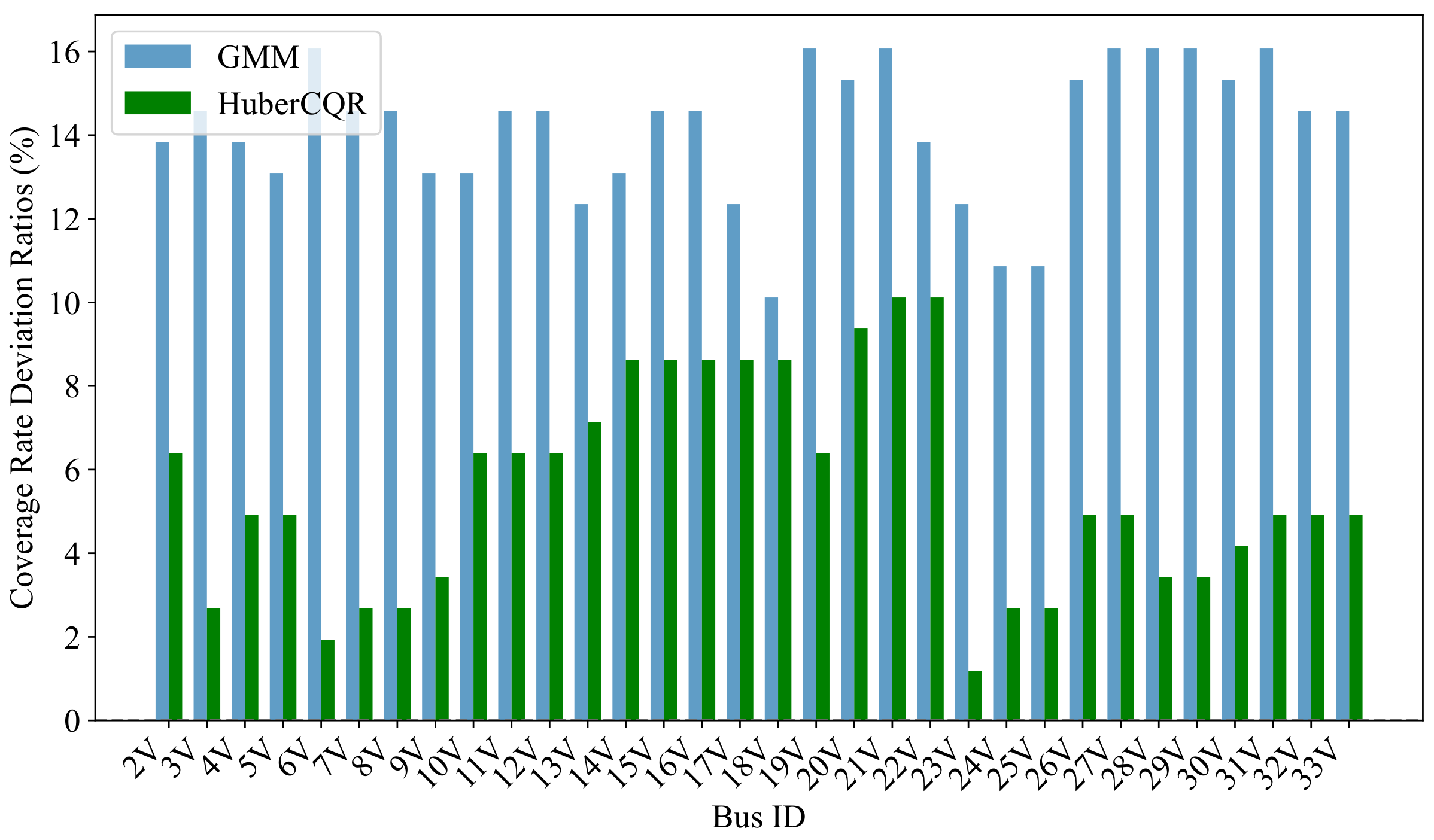
Figure 3 compares the Coverage Rate Deviation Ratio (CRDR) for the PatchTST model with the HuberCQR loss function and the GMM loss function. The CRDR is defined by Equation (28). A lower CRDR indicates that the actual coverage rate achieved by the model is closer to the theoretical 80% target, meaning the model is making more accurate predictions of the voltage fluctuation range:

Figure 3.
Coverage rate comparison under the two prediction models.
The figure shows that the CRDR for the HuberCQR-based PatchTST model is consistently lower across all non-reference buses compared to the GMM-based model. This suggests that the HuberCQR-based model performs better in prediction accuracy. This is crucial for making precise dispatch decisions for DESS, since the predicted and directly influence the operational limits of DESS through Equations (17) and (18).
4.2. Comparison of DESS Dispatch Results
After evaluating the accuracy of the coverage rates between two probabilistic prediction models, we utilize the predictions to guide the economic scheduling of DESS and compare the cost-effectiveness of the resulting schedules. Specifically, the predicted quantiles and are substituted into the DESS CCED model, and the chance constraints for addressing the probabilities of bus voltage violations can be transformed into solvable deterministic constraints.
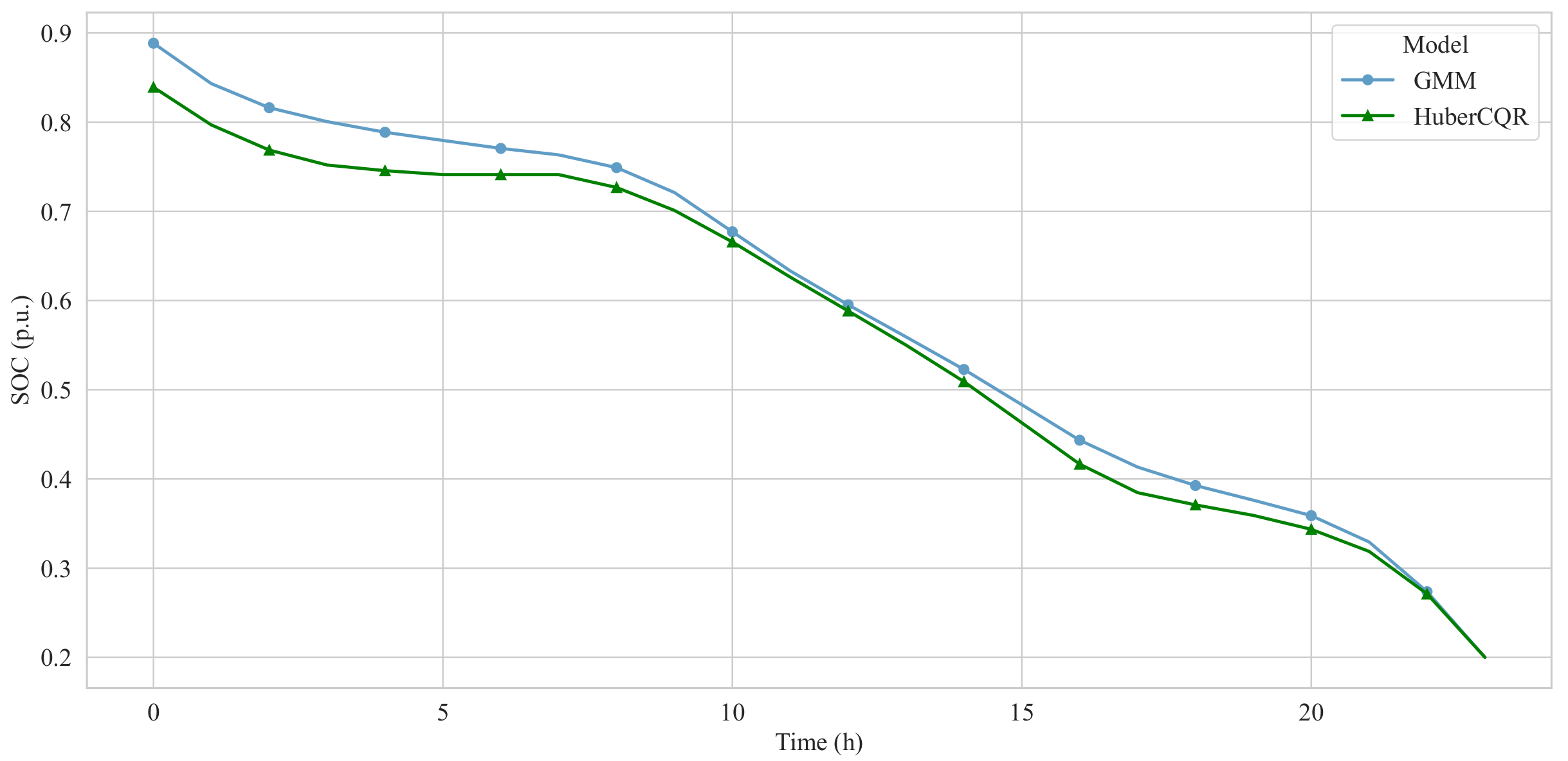
In the simulation, DESS integration bus is set to #18. Figure 4 shows that the more accurate estimation of bus voltage fluctuations under the HuberCQR-based PatchTST model leads to a lower DOD for the DESS, implying less degradation. The dispatch-related operating costs of the DESS further corroborate this point. Specifically, the daily dispatch cost based on the PatchTST model with the HuberCQR loss function is $1507.2 lower (a 6.23% reduction) compared to the cost based on the PatchTST model with the GMM loss function. The reduced operating cost highlights the practical benefits of the HuberCQR-based PatchTST model in optimizing DESS dispatch under uncertainty.

Figure 4.
DESS SOC dispatch results at bus #18.
4.3. Comparison of Bus Voltage
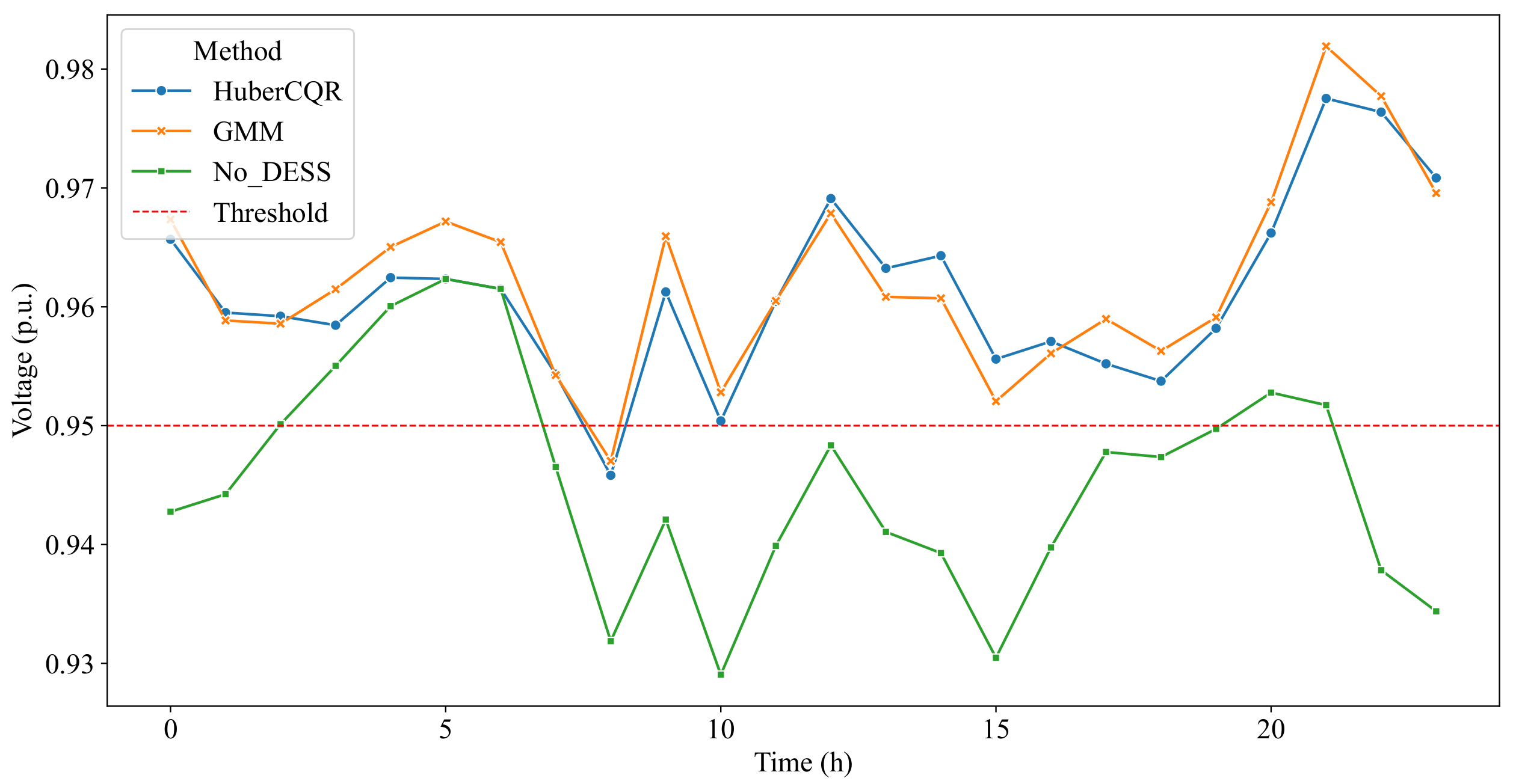
After obtaining the DESS scheduling results based on the two prediction models, we can compare the bus voltage conditions by combining the DESS scheduling results and the actual load data to verify whether the proposed methods have handled the chance constraints properly. Figure 5 shows the voltage conditions of bus #18 in the cases without DESS and with DESS dispatched based on the two prediction models. It can be seen that without DESS, the bus voltage is below the threshold most of the time. In contrast, with dispatching DESS under the two models, the probability of bus voltage exceeding the limits is less than setting , which is actually 0.04. This result reflects that both prediction models can well predict the risk of voltage fluctuation and fully utilize the capability of DESS in voltage management. Combining the results from the Section 4.2, it can be seen that the proposed scheduling scheme based on the HuberCQR prediction results can achieve the same effectiveness of voltage management as the scheme based on the GMM model, but with lower DESS scheduling costs.

Figure 5.
Voltage at bus #18.
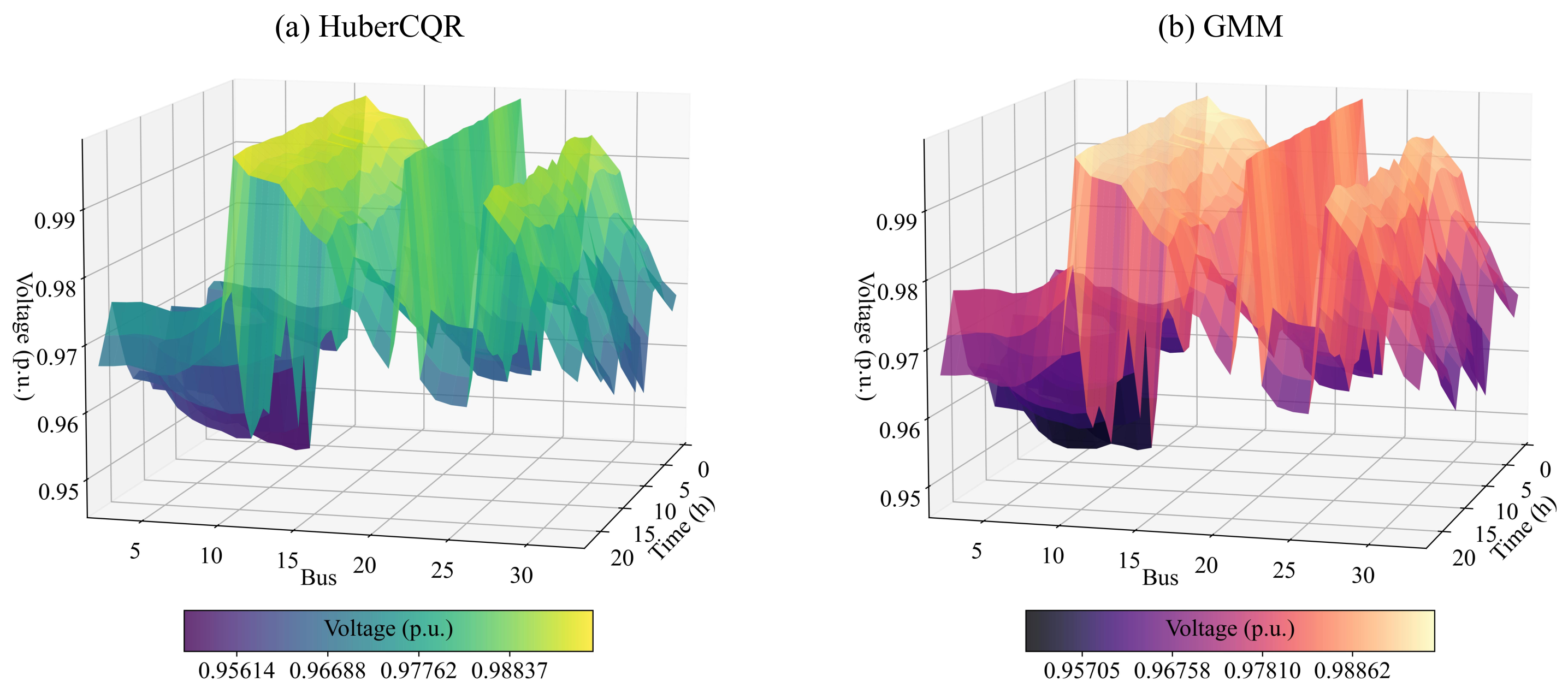
Furthermore, we analyze the 3D surface plots of the voltage levels under the cases under the HuberCQR-based and GMM-based model at different buses and time steps. It is observed from Figure 6 that the surface plot with the HuberCQR model shows a relatively smooth surface with fewer peaks and valleys, indicating that the predicted voltages are more stable across different buses and times. In contrast, the plot of the GMM model exhibits a more rugged surface with more pronounced peaks and valleys, suggesting that this model has a greater variance in voltage prediction. This result verifies that the performance of the HuberCQR-based model is consistent with its theoretical design, and it is more robust in predicting voltage fluctuations, with stronger ability to resist outlier risks.

Figure 6.
Three-dimensional surface plots of the voltage levels under the two prediction models.
5. Conclusions
As the types and scales of loads continue to increase, voltage issues in distribution networks become more pronounced. DESS can significantly mitigate the gradually intensifying voltage violation problems in distribution networks. Due to randomness and uncertainty of loads, the scheduling of DESS requires accurate prediction of the potential range of voltage fluctuations caused by random loads. Hence, this paper proposes a framework that combines deep learning with non-parametric probabilistic prediction method. Specifically, by utilizing a Transformer-based time series prediction model and an improved composite quantile regression technique, the DESS CCED problem considering voltage safety can be simplified into a feasible MILP problem, without the need for preset probability distributions of random variables and complex computations. Numerical experiments show that under the same voltage risk management effectiveness, the dispatching cost of DESS based on the proposed non-parametric probabilistic prediction model is lower than that based on state-of-the-art parametric models. Overall, this paper provides an efficient and economical solution for DESS dispatch considering load uncertainty and distribution network voltage safety. In the future, we hope to explore how prediction accuracy of the proposed model impacts the DESS scheduling results.
Author Contributions
Conceptualization, X.C. and T.Q.; methodology, X.C. and Y.Z.; software, X.C.; validation, X.C.; formal analysis, X.C. and Y.G.; investigation, X.C.; resources, X.C.; data curation, X.C.; writing—original draft preparation, X.C.; writing—review and editing, Y.G., Y.Z. and T.Q.; visualization, X.C.; supervision, Y.Z. and T.Q. All authors have read and agreed to the published version of the manuscript.
Funding
This research was funded by Jiangsu Provincial Key Research and Development Program (BE2020081-2), and by the Jiangsu Provincial Key Laboratory Project of Smart Grid Technology and Equipment.
Data Availability Statement
The code used in this study is available from the authors upon request.
Conflicts of Interest
The authors declare no conflicts of interest.
References
- Murray, W.; Adonis, M.; Raji, A. Voltage Control in Future Electrical Distribution Networks. Renew. Sustain. Energy Rev. 2021, 146, 111100. [Google Scholar] [CrossRef]
- Bendík, J.; Cenký, M.; Cintula, B.; Beláń, A.; Eleschová, Ž.; Janiga, P. Stochastic Approach for Increasing the PV Hosting Capacity of a Low-Voltage Distribution Network. Processes 2023, 11, 9. [Google Scholar] [CrossRef]
- Jabir, H.J.; Teh, J.; Ishak, D.; Abunima, H. Impacts of Demand-Side Management on Electrical Power Systems: A Review. Energies 2018, 11, 1050. [Google Scholar] [CrossRef]
- Abou El-Ela, A.A.; El-Sehiemy, R.A.; Salah Ali, E.; Kinawy, A.M. Minimisation of Voltage Fluctuation Resulted from Renewable Energy Sources Uncertainty in Distribution Systems. IET Gener. Transm. Distrib. 2019, 13, 2339–2351. [Google Scholar] [CrossRef]
- Zhang, D.; Li, J.; Hui, D. Coordinated Control for Voltage Regulation of Distribution Network Voltage Regulation by Distributed Energy Storage Systems. Prot. Control Mod. Power Syst. 2018, 3, 1–8. [Google Scholar] [CrossRef]
- Li, X.; Ma, R.; Gan, W.; Yan, S. Optimal Dispatch for Battery Energy Storage Station in Distribution Network Considering Voltage Distribution Improvement and Peak Load Shifting. J. Mod. Power Syst. Clean Energy 2020, 10, 131–139. [Google Scholar] [CrossRef]
- Han, R.; Hu, Q.; Cui, H.; Chen, T.; Quan, X.; Wu, Z. An optimal bidding and scheduling method for load service entities considering demand response uncertainty. Appl. Energy 2022, 328, 120167. [Google Scholar] [CrossRef]
- Kheirkhah, A.R.; Meschini Almeida, C.F.; Kagan, N.; Leite, J.B. Optimal Probabilistic Allocation of Photovoltaic Distributed Generation: Proposing a Scenario-Based Stochastic Programming Model. Energies 2023, 16, 7261. [Google Scholar] [CrossRef]
- Ramadan, A.; Ebeed, M.; Kamel, S.; Abdelaziz, A.Y.; Haes Alhelou, H. Scenario-Based Stochastic Framework for Optimal Planning of Distribution Systems Including Renewable-Based DG Units. Sustainability 2021, 13, 3566. [Google Scholar] [CrossRef]
- Jeddi, B.; Vahidinasab, V.; Ramezanpour, P.; Aghaei, J.; Shafie-khah, M.; Catalão, J.P. Robust Optimization Framework for Dynamic Distributed Energy Resources Planning in Distribution Networks. Int. J. Electr. Power Energy Syst. 2019, 110, 419–433. [Google Scholar] [CrossRef]
- Sun, Q.; Chen, Q. Fully Decentralized Robust Modelling and Optimization of Radial Distribution Networks Considering Uncertainties. IEEE Trans. Smart Grid 2021, 13, 1012–1022. [Google Scholar] [CrossRef]
- Cao, Y.; Tan, Y.; Li, C.; Rehtanz, C. Chance-Constrained Optimization-Based Unbalanced Optimal Power Flow for Radial Distribution Networks. IEEE Trans. Power Deliv. 2013, 28, 1855–1864. [Google Scholar]
- Nazir, F.U.; Pal, B.C.; Jabr, R.A. A Two-Stage Chance Constrained Volt/Var Control Scheme for Active Distribution Networks with Nodal Power Uncertainties. IEEE Trans. Power Syst. 2018, 34, 314–325. [Google Scholar] [CrossRef]
- Zhang, J.; Cheng, C.; Yu, S.; Su, H. Chance-Constrained Co-Optimization for Day-Ahead Generation and Reserve Scheduling of Cascade Hydropower—Variable Renewable Energy Hybrid Systems. Appl. Energy 2022, 324, 119732. [Google Scholar] [CrossRef]
- Zhang, Z.S.; Sun, Y.Z.; Gao, D.W.; Lin, J.; Cheng, L. A Versatile Probability Distribution Model for Wind Power Forecast Errors and Its Application in Economic Dispatch. IEEE Trans. Power Syst. 2013, 28, 3114–3125. [Google Scholar] [CrossRef]
- Yu, J.; Li, Z.; Guo, Y.; Sun, H. Decentralized Chance-Constrained Economic Dispatch for Integrated Transmission-District Energy Systems. IEEE Trans. Smart Grid 2019, 10, 6724–6734. [Google Scholar] [CrossRef]
- Wan, C.; Lin, J.; Wang, J.; Song, Y.; Dong, Z.Y. Direct Quantile Regression for Nonparametric Probabilistic Forecasting of Wind Power Generation. IEEE Trans. Power Syst. 2016, 32, 2767–2778. [Google Scholar] [CrossRef]
- Akhavan-Hejazi, H.; Mohsenian-Rad, H. Energy Storage Planning in Active Distribution Grids: A Chance-Constrained Optimization with Non-Parametric Probability Functions. IEEE Trans. Smart Grid 2016, 9, 1972–1985. [Google Scholar]
- Qian, T.; Ming, W.; Shao, C.; Hu, Q.; Wang, X.; Wu, J.; Wu, Z. An Edge Intelligence-Based Framework for Online Scheduling of Soft Open Points With Energy Storage. IEEE Trans. Smart Grid 2023. Early Access. [Google Scholar] [CrossRef]
- Qian, T.; Shao, C.; Wang, X.; Shahidehpour, M. Deep reinforcement learning for EV charging navigation by coordinating smart grid and intelligent transportation system. IEEE Trans. Smart Grid 2019, 11, 1714–1723. [Google Scholar] [CrossRef]
- Qian, T.; Shao, C.; Shi, D.; Wang, X.; Wang, X. Automatically Improved VCG Mechanism for Local Energy Markets via Deep Learning. IEEE Trans. Smart Grid 2021, 13, 1261–1272. [Google Scholar] [CrossRef]
- Shi, H.; Xu, M.; Li, R. Deep Learning for Household Load Forecasting-A Novel Pooling Deep RNN. IEEE Trans. Smart Grid 2017, 9, 5271–5280. [Google Scholar] [CrossRef]
- Zhu, J.; Yang, Z.; Mourshed, M.; Guo, Y.; Zhou, Y.; Chang, Y.; Wei, Y.; Feng, S. Electric Vehicle Charging Load Forecasting: A Comparative Study of Deep Learning Approaches. Energies 2019, 12, 2692. [Google Scholar] [CrossRef]
- Li, Z.; Li, Y.; Liu, Y.; Wang, P.; Lu, R.; Gooi, H.B. Deep Learning Based Densely Connected Network for Load Forecasting. IEEE Trans. Power Syst. 2020, 36, 2829–2840. [Google Scholar] [CrossRef]
- Zhang, Y.; Qian, W.; Ye, Y.; Li, Y.; Tang, Y.; Long, Y.; Duan, M. A Novel Non-Intrusive Load Monitoring Method Based on ResNet-Seq2Seq Networks for Energy Disaggregation of Distributed Energy Resources Integrated with Residential Houses. Appl. Energy 2023, 349, 121703. [Google Scholar] [CrossRef]
- Nie, Y.; Nguyen, N.H.; Sinthong, P.; Kalagnanam, J. A Time Series Is Worth 64 Words: Long-Term Forecasting with Transformers. arXiv 2022, arXiv:2211.14730. [Google Scholar]
- Meyer, G.P. An alternative probabilistic interpretation of the Huber loss. In Proceedings of the IEEE/CVF Conference on Computer Vision and Pattern Recognition (CVPR), Online. 19–25 June 2021; pp. 5261–5269. [Google Scholar]
- Huber, P.J. Robust estimation of a location parameter. In Breakthroughs in Statistics: Methodology and Distribution; Springer: New York, NY, USA, 1992; pp. 492–518. [Google Scholar]
- Zou, H.; Yuan, M. Composite Quantile Regression and the Oracle Model Selection Theory. Ann. Statist. 2008, 36, 1108–1126. [Google Scholar] [CrossRef]
- Kashem, M.A.; Ganapathy, V.; Jasmon, G.B.; Buhari, M.I. A Novel Method for Loss Minimization in Distribution Networks. In Proceedings of the DRPT2000. International Conference on Electric Utility Deregulation and Restructuring and Power Technologies, London, UK, 4–7 April 2000; pp. 251–256. [Google Scholar]
- Baran, M.E.; Wu, F.F. Network Reconfiguration in Distribution Systems for Loss Reduction and Load Balancing. IEEE Trans. Power Deliv. 1989, 4, 1401–1407. [Google Scholar] [CrossRef]
- Farivar, M.; Chen, L.; Low, S. Equilibrium and dynamics of local voltage control in distribution systems. In Proceedings of the 52nd IEEE Conference on Decision and Control, Firenze, Italy, 10–13 December 2013; pp. 4329–4334. [Google Scholar]
- Zheng, Y.; Zhao, J.; Song, Y.; Luo, F.; Meng, K.; Qiu, J.; Hill, D.J. Optimal Operation of Battery Energy Storage System Considering Distribution System Uncertainty. IEEE Trans. Sustain. Energy 2017, 9, 1051–1060. [Google Scholar] [CrossRef]
- Koenker, R.; Bassett, G., Jr. Regression Quantiles. Econom. J. Econ. Soc. 1978, 46, 33–50. [Google Scholar] [CrossRef]
- Quesada, C.; Astigarraga, L.; Merveille, C.; Borges, C.E. An electricity smart meter dataset of Spanish households: Insights into consumption patterns. Sci Data 2024, 11, 59. [Google Scholar] [CrossRef] [PubMed]
- Liu, G.; Sun, W.; Hong, H.; Shi, G. Coordinated Configuration of SOPs and DESSs in an Active Distribution Network Considering Social Welfare Maximization. Sustainability 2024, 16, 2247. [Google Scholar] [CrossRef]
Disclaimer/Publisher’s Note: The statements, opinions and data contained in all publications are solely those of the individual author(s) and contributor(s) and not of MDPI and/or the editor(s). MDPI and/or the editor(s) disclaim responsibility for any injury to people or property resulting from any ideas, methods, instructions or products referred to in the content. |
© 2024 by the authors. Licensee MDPI, Basel, Switzerland. This article is an open access article distributed under the terms and conditions of the Creative Commons Attribution (CC BY) license (https://creativecommons.org/licenses/by/4.0/).