Article

A Deep Learning Approach Based on Novel Multi-Feature Fusion for Power Load Prediction

1
School of Mathematics and Statistics, Xuzhou University of Technology, Xuzhou 221018, China
2
Faculty of Science and Technology, University of Macau, Taipa, Macau 999078, China
3
School of Economics and Management, Chongqing University of Posts and Telecommunications, Chongqing 400065, China
*
Author to whom correspondence should be addressed.
Processes 2024, 12(4), 793; https://doi.org/10.3390/pr12040793
Submission received: 18 March 2024 / Revised: 5 April 2024 / Accepted: 10 April 2024 / Published: 15 April 2024

Abstract

:
Adequate power load data are the basis for establishing an efficient and accurate forecasting model, which plays a crucial role in ensuring the reliable operation and effective management of a power system. However, the large-scale integration of renewable energy into the power grid has led to instabilities in power systems, and the load characteristics tend to be complex and diversified. Aiming at this problem, this paper proposes a short-term power load transfer forecasting method. To fully exploit the complex features present in the data, an online feature-extraction-based deep learning model is developed. This approach aims to extract the frequency-division features of the original power load on different time scales while reducing the feature redundancy. To solve the prediction challenges caused by insufficient historical power load data, the source domain model parameters are transferred to the target domain model utilizing Kendall’s correlation coefficient and the Bayesian optimization algorithm. To verify the prediction performance of the model, experiments are conducted on multiple datasets with different features. The simulation results show that the proposed model is robust and effective in load forecasting with limited data. Furthermore, if real-time data of new energy power systems can be acquired and utilized to update and correct the model in future research, this will help to adapt and integrate new energy sources and optimize energy management.

1. Introduction

1.1. Background and Challenges

Global warming triggered by greenhouse gases presents an environmental challenge to humanity [1].As the world’s largest developing country, China proposed the “Carbon Peaking and Carbon Neutrality” goals to reduce carbon emissions in 2020. The power sector accounts for more than 1/3 of the national carbon emissions in China. Therefore, exploring and utilizing new energy sources to generate electricity have become an essential solution for the decarbonization plan [2]. Owing to the vulnerability of this power generation type to weather conditions and geographical location, there is increased randomness and complexity in the power system [3]. Consequently, it is necessary to capture uncertainty caused by new energy grid connections using power load forecasting, which is conducive to the sustainable development of the power system. For example, ref. [4] used a novel stochastic short-term load forecasting technique using classifier regression mapping, and demonstrated its impact in power system management on a grid-connected multi-energy system. Ref. [5] proposed a probabilistic net load forecasting framework to unlock the potential of integrated energy systems by forecasting electricity demand, heat demand, and photovoltaic generation. Ref. [6] proposed an ensemble-based short-term load forecasting method tailored for buildings, which was applied to predict future energy demands and manage the intermittency and variability of renewable energy sources.

1.2. Knowledge Gaps

Even though a lot of researchers have devoted their efforts to power load prediction, there are still several knowledge gaps in load power prediction research, which can be listed as follows.
Firstly, inadequate consideration of the online features in the power load series can easily lead to difficulties in adapting the model to dynamic changes in the data. Although the existed models are used for mining frequency-division features and adjusting model parameters in real time, no specific details about their implementation, algorithms, or technical aspects are provided. Further descriptions would help us to understand the working principles and practical application scenarios of the models.
Secondly, the lack of limited dataset techniques may expose forecast results to a dilemma, making them unable to provide reliable information for decision making. Obtaining accurate and comprehensive data on historical load patterns, weather conditions, demographic factors, and other relevant variables is a challenge for researchers. Limited data might make accurately capturing the complex non-linear relationships between the load and influencing factors difficult.

1.3. The Model Proposed in This Work

To enable a model to automatically extract features, deep learning is generally employed, considering that hybrid deep learning models can make full use of the advantages of different neural networks and thus strengthening the performance and generalization of the model. Therefore, this paper couples a convolutional neural network (CNN) and bi-directional long short-term memory (BiLSTM) in a prediction model. In detail, the CNN extracts deep local features in power load sequences, which are then sent to the BiLSTM layer to strengthen the connection between temporal features.
The power load forecasting procedures will be divided into a training procedure, a validation procedure, and a testing procedure. In the training procedure, the training set is utilized to train the network parameters of the model so that it can recognize data features and patterns. In the validation procedure, the validation set is used to adjust the hyperparameters of the model. During the training process, the Bayesian optimization algorithm is introduced to dynamically set the hyperparameters according to the different features of the input sequences, which improves the prediction accuracy of the model. In the test procedure, the test set is used to evaluate the prediction performance of the model on unfamiliar data as a way of checking the generalization ability of the model.
In addition, taking into account the nonlinearity, non-stationarity, and accessibility of power load data, especially under a high proportion of new energy sources connected to the grid, this paper will introduce empirical modal decomposition based on time-varying filtering and transfer learning to address the challenges that may be faced by power load forecasting work.

1.4. Novelty and Contributions

Aiming at addressing the knowledge gaps above, a novel hybrid load forecasting model, cooperating with an online data processing model and transfer learning, is proposed to forecast the short-term power load with a limited dataset. An online data processing model is proposed to solve the problem of insufficient frequency-division feature extraction. Concretely, a novel feature decomposition–reorganization method is used to diversify and reorganize online features. A hybrid deep learning framework is constructed to train the model and determine the optimal parameters of the model according to the different features. Furthermore, a framework based on transfer learning is applied to solve the problem of insufficient historical load data. The main contributions of this paper are summarized below:
(1) Since power loads are characterized by different frequency bands overlapping each other, an online data processing model is proposed to mine frequency-division features at different time steps. It can adjust the model parameter settings in real time using the different characteristics of load series so that the forecasting performance can be effectively improved.
(2) To resolve the problem of historical power load inadequacy, the proposed forecasting model based on transfer learning is applied to a limited dataset. Before transferring the model, Kendall’s coefficient is introduced to assess transferability among datasets, which can avoid negative migration. Experimental results on the limited dataset show that the method can significantly decrease the forecasting error on the limited dataset.
(3) A hybrid forecasting deep learning framework is constructed, which combines an intelligent optimization algorithm, a modal decomposition technique, and transfer learning. To validate the reliability and generalization of the proposed forecasting model, experiments are conducted on multiple datasets with different features, and the results are compared with current popular prediction models. The experimental results of the proposed model have a higher accuracy and better stability.

2. Literature Review

Relevant research indicates that power load forecasting techniques can be divided into classical statistical methods, machine learning methods, and hybrid models based on deep learning. Classical statistical methods, such as regression analysis [7], exponential smoothing [8], auto-regressive integrated moving average [9], and the gray model [10], have a simple structure. However, these models require strict smoothness of the input data and cannot explain the various nonlinear factors affecting the power load. Traditional machine learning techniques have been proposed to learn nonlinear relationships, such as support vector machine [11] and extreme learning machine [12]. They can only learn shallow features, while deep learning can dig deeper into the temporal features [13]. For example, due to the complex implicit layer and loop structure, gated recurrent units, long short-term memory (LSTM), and BiLSTM mine deeper features from power loads.
In recent years, hybrid models based on deep learning have been widely used in the field of load forecasting. In comparison to a single neural network, the coupling of multiple neural networks, especially the coupling of a CNN and other networks, can improve the generalization ability and forecasting accuracy [14]. For example, ref. [15] combined a CNN and LSTM in a prediction model with an attention mechanism, and applied it to short-term power load forecasting. As one of the most popular models in load forecasting, BiLSTM is trained to utilize both sequential and reverse-time direction information to obtain more data features [16]. Therefore, it is meaningful to couple a CNN and BiLSTM to predict future power load trends.
Feature extraction plays a crucial role in deep learning models to recognize and learn load randomness and volatility features. Since the high percentage of new energy grid connections has increased the volatility and uncertainty of power loads, it is highly challenging to extract valid features in depth. To obtain more rich and valuable information, some scholars utilize feature extraction methods to decompose the time subsequence into multiple sub-sequences [17]. Representative methods, including empirical modal decomposition (EMD) [18], ensemble empirical mode decomposition [19] and variational modal decomposition [20], are widely used in the field of power load forecasting. The above methods may suffer from the modal mixing problem, the final averaging problem, and poor parameter self-adaptation [21]. By construct, time-varying filtering-based EMD (TVFEMD) can mitigate the modal mixing problem and has strong robustness to noise interference. Ref. [22] applied TVFEMD to wind speed forecasting and achieved the desired prediction accuracy. Moreover, TVFEMD is rarely used in the field of power load forecasting. Therefore, TVFEMD is applied to reduce the volatility of the raw power load in this paper to mine frequency-division features at different time steps. In addition, to avoid the computational burden and information redundancy caused by excessive decomposition, sample entropy theory is applied in this paper.
Additionally, most researchers focus on how well the forecasting models fit at the data level, providing that a sufficiently large dataset is available. However, due to the high cost of manual annotation and the noise in raw data, there are often insufficient sample data in practice [23]. A limited training dataset is prone to overfitting deep learning models, resulting in a sub-optimal prediction accuracy. The latest research suggests that transfer learning can solve the above problems, and it has a large number of successful applications in the field of energy prediction [24,25]. In detail, transfer learning takes the knowledge gained from one domain containing a rich training dataset and uses it to solve problems in the target domain. For example, ref. [26] described a transfer learning model based on the attention mechanism, which utilized similar building datasets to enhance the predictive accuracy for new buildings with the limited dataset. Ref. [27] presented an approach based on a modified K-means method combined with a mutual information feature selection algorithm, XGBoost, and transfer learning; the experimental results show that using knowledge learned from other domains reduces the prediction errors. Therefore, considering the scarcity of historical power load data, it is necessary to study the load forecasting accuracy of deep learning models combined with transfer learning.

3. Methodology

The model proposed in this paper is applied to short-term electricity load forecasting, which combines the theoretical knowledge of TVFEMD, sample entropy, CNN, BiLSTM and the Bayesian optimization algorithm. Therefore, the theoretical knowledge of the used methods is carefully introduced in Section 3.1Section 3.4, while Section 3.5 describes the prediction framework and the specific implementation of the proposed prediction model.

3.1. Time-Varying Filter-Based EMD

Time-varying filter-based empirical mode decomposition was proposed to alleviate the aliasing mode problem [28]. In EMD, the estimation of the local average is viewed as a linear filter with a constant local cutoff frequency, which makes it difficult to deal with nonlinear and nonsmooth signals. In contrast, TVFEMD adopts the B-spline approximation as a filter with a time-varying cutoff frequency. The biggest improvements of TVFEMD are that it makes full use of the instantaneous amplitude and instantaneous frequency, it adaptively designs the local cut-off frequency, and then it decomposes the original signal into local high-frequency series and local low-frequency series. The implementation process of TVFEMD is as follows.
Perform the Hilbert transform on the original signal  D ( t ) ; the result is denoted by  D ˜ ( t ) . Then, calculate the instantaneous amplitude  A ( t )  and instantaneous phase  φ ( t ) .
A ( t ) = D ( t ) 2 + D ˜ ( t ) 2
φ ( t ) = arctan D ˜ ( t ) / D ( t )
Find out the local maximum sequence and local minimum sequence of  A ( t ) , expressed as  A t m i n  and  A t m a x , respectively.
Interpolate  A t m i n  and  A t m a x , respectively, to estimate  μ 1 ( t )  and  μ 2 ( t ) . The instantaneous amplitudes  α 1 ( t )  and  α 2 ( t )  can be obtained via Equations (3) and (4).
α 1 ( t ) = μ 1 ( t ) + μ 2 ( t ) / 2
α 2 ( t ) = μ 2 ( t ) μ 1 ( t ) / 2
Interpolate  A t m a x 2 φ t m a x  and  A t m i n 2 φ t m i n  to obtain  δ 1 t  and  δ 2 t , respectively. The instantaneous frequencies  φ 1 ( t )  and  φ 2 ( t )  can be computed by Equations (5) and (6).
φ 1 ( t ) = δ 1 ( t ) 2 α 1 2 ( t ) 2 α 1 ( t ) α 2 ( t ) + δ 2 ( t ) 2 α 1 2 ( t ) + 2 α 1 ( t ) α 2 ( t )
φ 2 ( t ) = δ 1 ( t ) 2 α 2 2 ( t ) 2 α 1 ( t ) α 2 ( t ) + δ 2 ( t ) 2 α 2 2 ( t ) + 2 α 1 ( t ) α 2 ( t )
The local cut-off frequency  φ b i a s ( t )  can be rearranged by solving Equation (7) to address the intermittence problem.
φ b i a s ( t ) = φ 1 ( t ) + φ 2 ( t ) 2 = δ 2 ( t ) δ 1 ( t ) 4 α 1 ( t ) α 2 ( t )
After obtaining a local cut-off frequency  φ b i a s ( t ) , calculate the signal  ( t ) .
( t ) = cos φ b i a s ( t ) d ( t )
Then, perform the B-spline approximate filter on  x ( t )  by taking the local extreme points  t m i n  and  t m a x  of  ( t )  as nodes, the approximate result denoted  m 1 ( t ) .
A stop criterion is defined here.
ζ ( t ) = B L o u g h l i n ( t ) φ a v g ( t )
If  ζ ( t ) τ D ( t )  is treated as an intrinsic mode function; otherwise,  D ( t ) m 1 ( t )  will be used as a new input signal, and the above steps are repeated. The bandwidth threshold  τ  is set to 0.1,  φ a v g ( t )  denotes the weighted average of instantaneous frequencies, and  B L o u g h l i n ( t )  represents the Loughlin instantaneous bandwidth.
Finally, the original signal  D ( t )  is decomposed via TVFEMD to obtain s components as  m i ( t ) | i = 1 , 2 , , s , satisfying
D ( t ) = i = 1 s m i ( t )

3.2. Sample Entropy

Sample entropy (SE) was proposed to measure the probability of generating a new pattern of the original signal [29], and reflects the complexity and irregularity of the time series. The greater the probability of a new pattern, the higher the complexity of the sequence and the greater the entropy value. On the contrary, the lower the probability of a new pattern, the lower the complexity of the sequence and the lower the entropy value. Theoretically, the sample entropy of the time series is formulated as follows:
S a m p E n = I n B ε ϖ + 1 ( t ) B ε ϖ ( t )
where  ϖ  is the reconstruction dimension,  ε  represents the similarity tolerance, with its value set to 0.1, and  B ε ϖ ( t )  is the probability of two sequences matching  ϖ  points under  ε .

3.3. Convolutional Neural Network

A CNN is a deep feedforward neural network which can extract deep local features from multi-dimensional inputs with sparse connections and parameter sharing [30]. To effectively extract and compress data features, the CNN in this paper is composed of two convolution layers, one pooling layer, and a flattening operation. In particular, Elu activation and maximum pooling functions are selected during neural network training.
The convolution layer extracts valid information from the input data through Equation (12).
c o n t = F ( w x t + b )
where  x t  is the t-th input date,  c o n t  is the output feature map of the -th convolution kernel, F is the activation function, w and b are, respectively, the weight matrix and bias of -th convolution kernel, and ⊗ is the sign of the convolution operation.
The pooling layer compresses the output features of the convolutional layer to generate more important information  ϱ t , implemented as in Equation (13).
ϱ t = m a x ( c o n t )

3.4. Bi-Directional Long Short-Term Memory

For the purpose of avoiding gradient disappearance and explosion problems, LSTM is used to extract historical information from power load data [31]. The network is made up of three gates, namely the input gate, the output gate, and the forgetting gate, and the memory cell’s state. Specifically, the memory cell selectively “forgets” and “remembers” information through the Sigmoid activation function and the point-by-point multiplication operation [32].
The forgetting gate  f t  determines what information is discarded from memory cell  c t 1 .
f t = σ ( w f ϱ t , h t 1 + b f )
The input gate  i t  determines what new information is added to the memory cell  c t .
i t = σ ( w i ϱ t , h t 1 + b i )
c ^ t = tanh ( w c ϱ t , h t 1 + b c )
c t = f t c t 1 + i t c ^ t
The output gate  o t  determines what important information is output.
o t = σ ( w o ϱ t , h t 1 + b o )
h t = o t tanh ( c t )
Since the LSTM propagates data from front to back in chronological order, it is difficult to learn the internal features of the data in depth. BiLSTM integrates a forward LSTM layer and a backward LSTM layer, enabling historical and future information generated by the hidden layers to be recursive and feedback towards the neural network [33]. The updated states of the forward LSTM and backward LSTM hidden layers and the final output process are calculated as follows:
h t = L S T M ( ϱ t , h t 1 )
H t = L S T M ( ϱ t , H t 1 )
y t = a f h t + a b H t + b t
where  σ  and  t a n h  denote the Sigmoid function,  w f w i w c , and  w o  are the weights matrices,  b f b i b c b o , and  b t  are the corresponding bias vectors, ⊙ is the point-by-point multiplication operation, and  h t 1  and  h t  indicate the output of the previous and current cells in the forward layer, respectively. LSTM is the operation of the traditional LSTM network and  H t  denotes the output of backward hidden layers.  a f  and  a b  are the output weights of the hidden layers of the forward and backward propagation units, respectively.

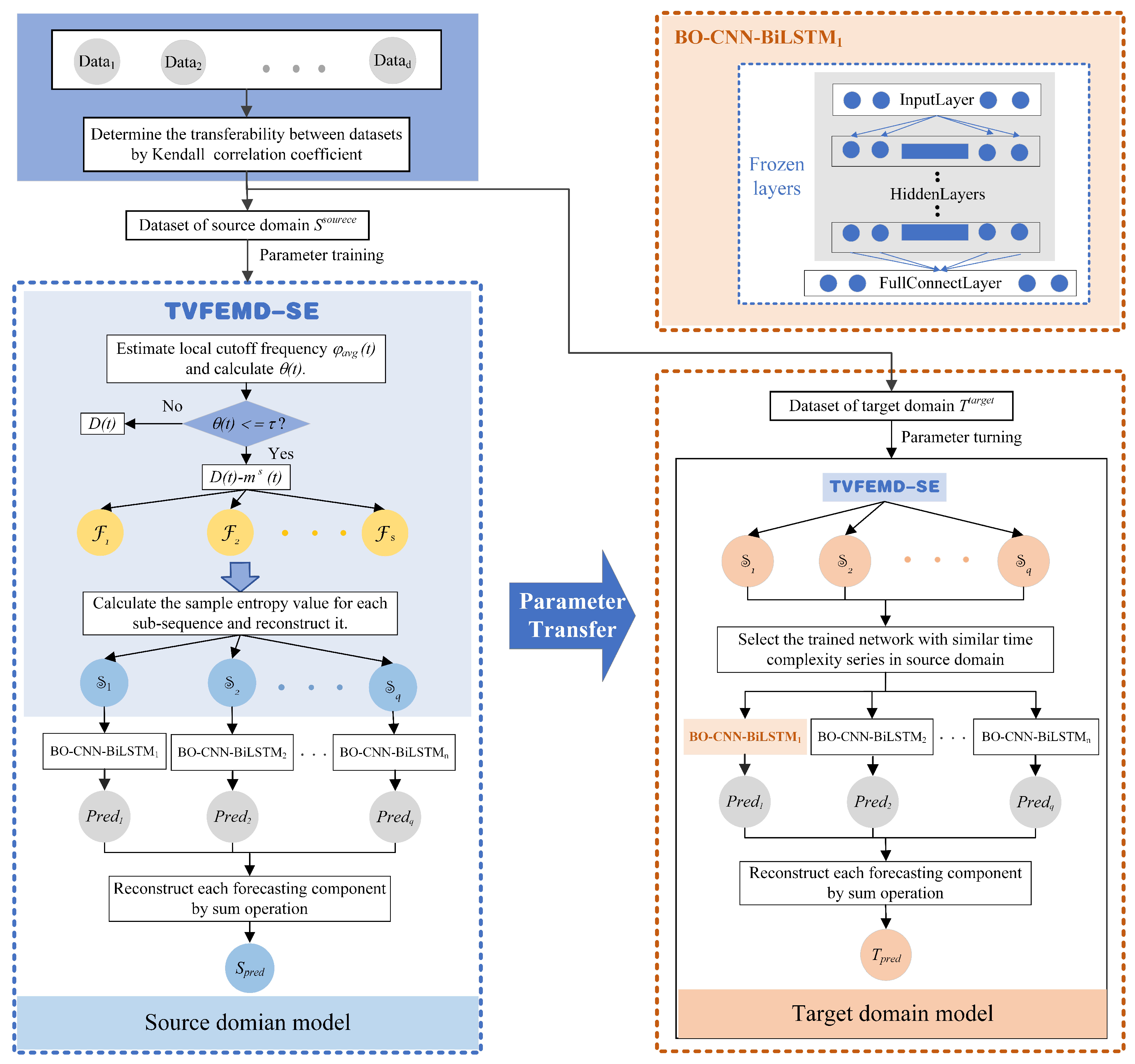
3.5. The Proposed Hybrid Model in This Study

This study proposes a hybrid model combining dynamic feature extraction methods, called TVFEMD-BO-CNN-BiLSTM, with transfer learning for short-term power load forecasting (shown in Algorithm 1 and Figure 1). Figure 1 illustrates the forecasting framework of the proposed model in this paper for electricity load. First, in the blue boxes of the top left part, the source domain dataset and target domain datasets are identified and applied to the corresponding model. Then, the blue dashed box of the lower left part (source domain model) aims to migrate the trained biases and weights into the orange dashed box of the lower right (target domain model). In this case, the migrated CNN-BiLSTM network layer parameters are detailed as shown in the upper-right orange box, including the input layer and the hidden layer. The gray-shaded portion is for freezing and migrating the network layer parameters in the source domain model into the target domain model. Algorithm 1 shows the specific operation and implementation of the prediction framework in Figure 1. The proposed model aims to mine frequency-division features at different time steps adopting the TVFEMD approach, and then, BO-CNN-BiLSTM is constructed to recognize and learn sub-sequence features; moreover, the hyperparameters of the proposed model are searched for different features of the input sequences. The proposed model is transferred to deal with limited datasets, and Kendall’s correlation coefficient is introduced to assess the transferability between the datasets.
This study adopts the TVFEMD method to decompose load data  D ( t ) = x t , y t t = 1 N  into several scales. At each data sampling time, apply the EMD method with a time-varying filter to the preprocessed data and obtain a real-time sequence of intrinsic mode functions (IMFs). Based on the real-time IMF sequence, features including frequency domain features, time domain features, and statistical features that can describe different aspects of the electrical load are extracted. At each new data sampling time, repeat the empirical mode decomposition and feature extraction steps with the latest real-time data. As new data enter, the feature values may change. To avoid learning redundant features, sample entropy is adopted to measure the complexity and irregularity of each IMF, IMFs with similar values of sample entropy are coalesced. In this way, the feature extraction process cannot only learn different frequencies adaptively, but also reduce the redundancy of calculations.
The CNN is adopted to recognize and learn the reconstructed sub-sequence features, and consists of an input layer, two convolutional layers, a maximum pooling layer, and a flattening operation. The convolutional layers extract the deep local features of input data, and the pooling layer compresses the extracted features into more critical information. BiLSTM consists of forward LSTM units and reverse LSTM units, which are used to learn temporal features extracted by the CNN to further mine long-term dependencies. Since the multiple reconstructed sub-sequences are characterized by different frequency bands, it is necessary to select appropriate parameters for different sequences dynamically in the CNN and BiLSTM networks. During the training process, the Bayesian optimization algorithm is employed to search for the optimal hyperparameters  Θ  by minimizing the loss function  L ( Θ ) . In order to choose the network parameters that minimize the prediction error, this study uses loss functions such as the root mean squared error (RMSE), mean absolute error (MAE), coefficient of determination ( R 2 ), and mean absolute percentage error (MAPE) to measure the difference between the true and forecasted values. This process of minimizing the loss functions is viewed as a multi-objective optimization problem.
To make the proposed model suitable for more scenarios, this study generalizes the proposed hybrid model to limited load datasets. The Kendall correlation coefficient ([34]) is introduced to calculate the similarity between the datasets  D a t a 1 , D a t a 2 , , D a t a d  to avoid negative transfer caused by a low or non-existent correlation between datasets in this study. The two datasets with the highest similarity are selected, and one is identified as  S s o u r c e  and the other as  T t a r g e t .
Algorithm 1 The pseudocode of the proposed model
Input:
Power load datasets:  D ( t ) = x t , y t t = 1 N .
The initial hyperparameters  Θ = θ 1 , θ 2 , , θ z .
Output:
Forecasting values:  T p r e d = y ^ t t = N + 1 N + k .
Accuracy: MAE,  R 2 , RMSE and MAPE
Optimal hyperparameters:  Θ * = θ 1 * , θ 2 * , , θ z * .
  1:
The calculated similarity coefficients between the datasets are evaluated to determine  S s o u r c e  and  T t a r g e t , let  S s o u r c e  be  D ( t ) = x t , y t t = 1 N .
  2:
Decompose power load series D into s sub-sequences, denoted as  F 1 t , F 2 t , , F s t t = 1 N .
  3:
Calculate the sample entropy according to Eq. (11) to measure the complexity of  F 1 t , F 2 t , , F s t t = 1 N .
  4:
Superimpose the decomposed sub-series with similar sample values to obtain the new series  S 1 t , S 2 t , , S q t t = 1 N .
  5:
Divide  S  into a training set, validation set and test set as  S = S t r a i n , S v a l i d , S t e s t .
  6:
Search for model hyperparameters with the Bayesian optimization algorithm, implemented as:
  7:
for  k = 1 , 2 , M a x i t e r  do
  8:
    Update the mean and variance of the posterior probability distribution.
  9:
    Construct the acquisition function  u ( Θ k 1 S t r a i n 1 : k 1 )  according to the mean and variance.
  10:
    Maximize  u ( Θ k 1 S t r a i n 1 : k 1 )  to determine the sampling point of the next iteration, denoted as  Θ k = a r g m a x u ( Θ k 1 S t r a i n 1 : k 1 ) .
  11:
    Obtain the loss function  L ( Θ k ) .
  12:
    Update the new dataset by adding point  [ Θ k , L ( Θ k ) ]  to the set  S t r a i n 1 : k .
  13:
    Update  Θ *  by objection function  L ( Θ * ) = min L ( Θ 1 ) , L ( Θ 2 ) , , L ( Θ k ) .
  14:
end for
  15:
return  Θ * = Θ 1 * , Θ 2 * , , Θ z * .
  16:
Input  S t e s t  into the source domain model  M s o u r c e  with  Θ *  to obtain a forecasted series  P r e d = P r e d 1 t , P r e d 2 t , , P r e d q t t = 1 N .
  17:
Superimpose  P r e d  to obtain the final forecast  S p r e d = y ^ t t = 1 N .
  18:
Calculate the accuracy to determine if the parameters in the network layers can be migrated. If the accuracy is ideal, transfer the parameters from  M s o u r c e  to the target domain model  M t a r g e t .
  19:
Let  T t a r g e t  be D, repeat steps 2 to 4 to process  T t a r g e t , and then put it into  M t a r g e t  to obtain the predicted values  T p r e d = y ^ t t = 1 N  according to steps 16 to 17.
The proposed model is trained on the source domain  S s o u r c e , and the optimal parameters of trained layers are saved. For the target domain  T t a r g e t , the input and hidden layers are frozen without updating their weights, and the parameters of the fully connection layer are trained with  T t a r g e t . Since the TVFEMD-SE algorithm divides load series into sequences with multiple frequency division features, selecting the network with a similar time complexity in the source domain is necessary to forecast future power loads.

4. Case Studies and Experimental Results

Two experiments are conducted in this section to demonstrate the performance of the proposed model; experiment I is conducted to validate the online feature extraction ability of the model, and experiment II verifies the performance of the model on the limited datasets.

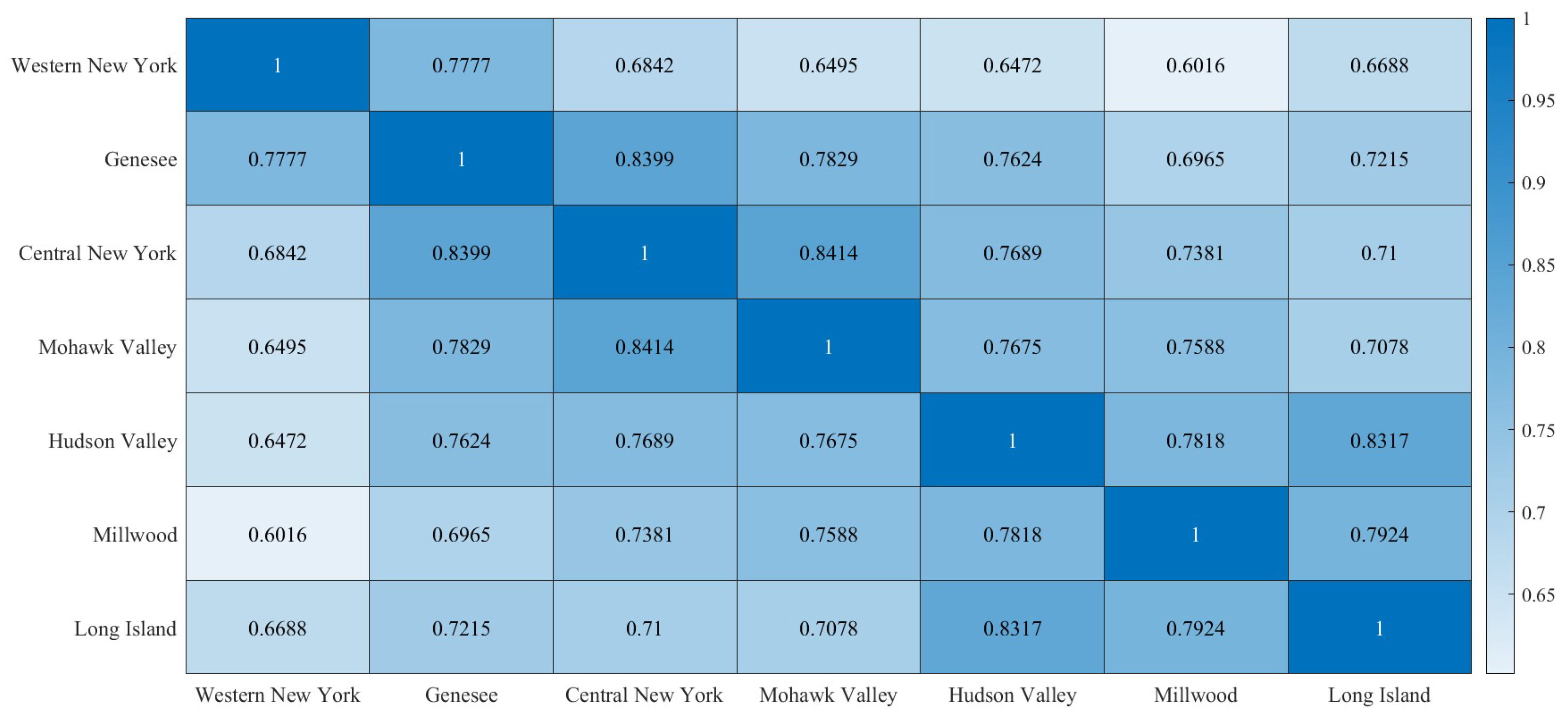
4.1. Data Sources and Descriptions

In the first experiment, two datasets are adopted. The first dataset is collected from a region of Australia (dataset 1), and the other dataset is collected from the 9th Electrician Mathematics Competition in China (dataset 2). Dataset 1 contains 8759 samples from January to December 2010, while Dataset 2 contains 8760 samples from January to December 2013. All sample points were collected every hour and divided into three parts, including the training set, validation set, and test set.
In the second experiment, the power load datasets from New York State divisions are selected, including Western New York, Genesee, Central New York, Mohawk Valley, Hudson Valley, Millwood, and Long Island, which were obtained from the New York Independent System Operator (NYISO). These datasets contain hourly power loads from January to December 2019.

4.2. Performance Metrics

To quantitatively assess the performance of different models, four indicators are selected, including the MAPE, RMSE, MAE, and  R 2 , which are mathematically defined as follows:
M A P E = 1 N t = 1 N y t y ^ t y t
R M S E = 1 N t = 1 N ( y t y ^ t ) 2
M A E = 1 N t = 1 N y t y ^ t
R 2 = 1 t = 1 N ( y t y ^ t ) 2 t = 1 N ( y t y ¯ t ) 2
where N is the number of sampling points and  y t y ¯ t , and  y ^ t  denote the actual values, average values, and forecasted values of the power load, respectively.

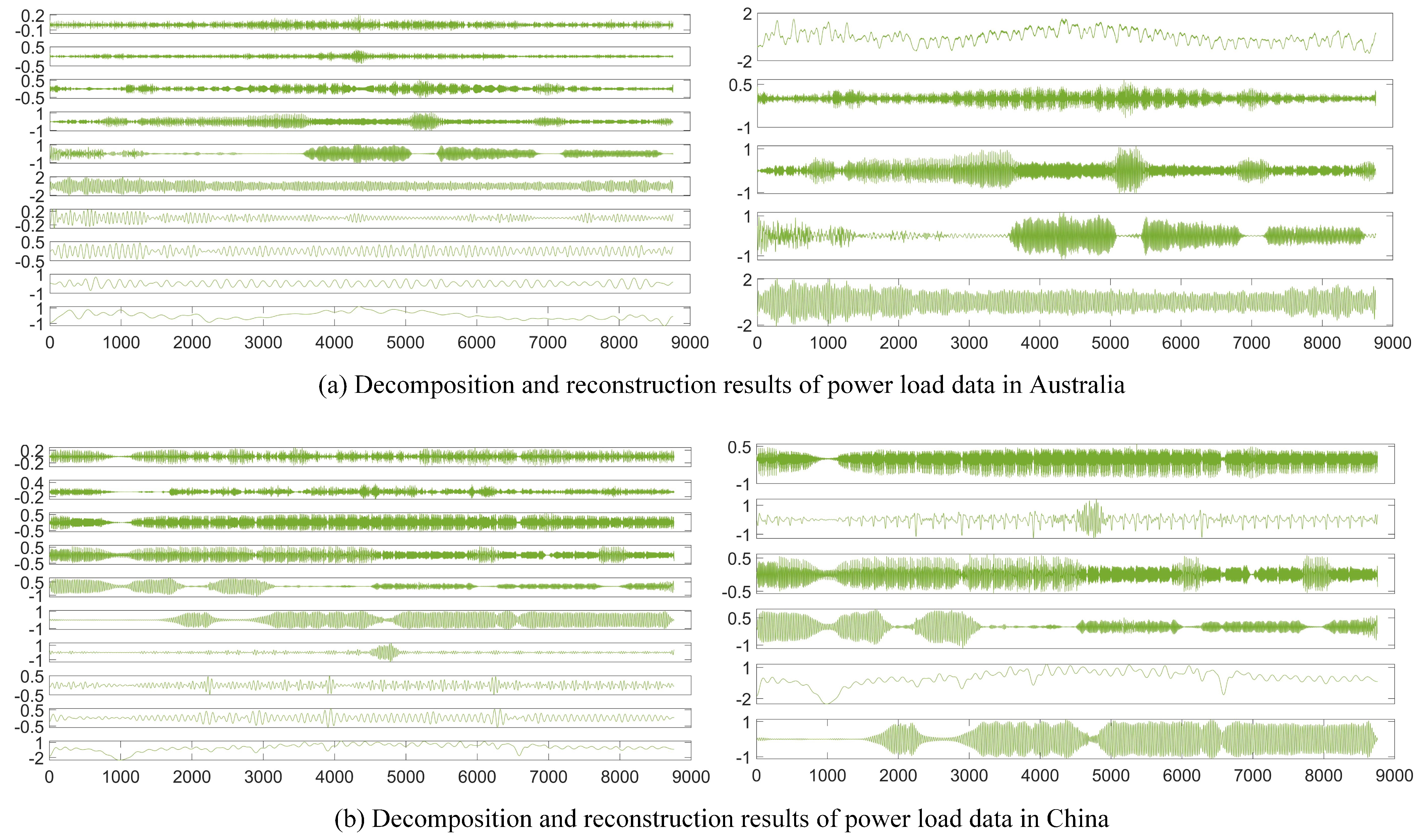
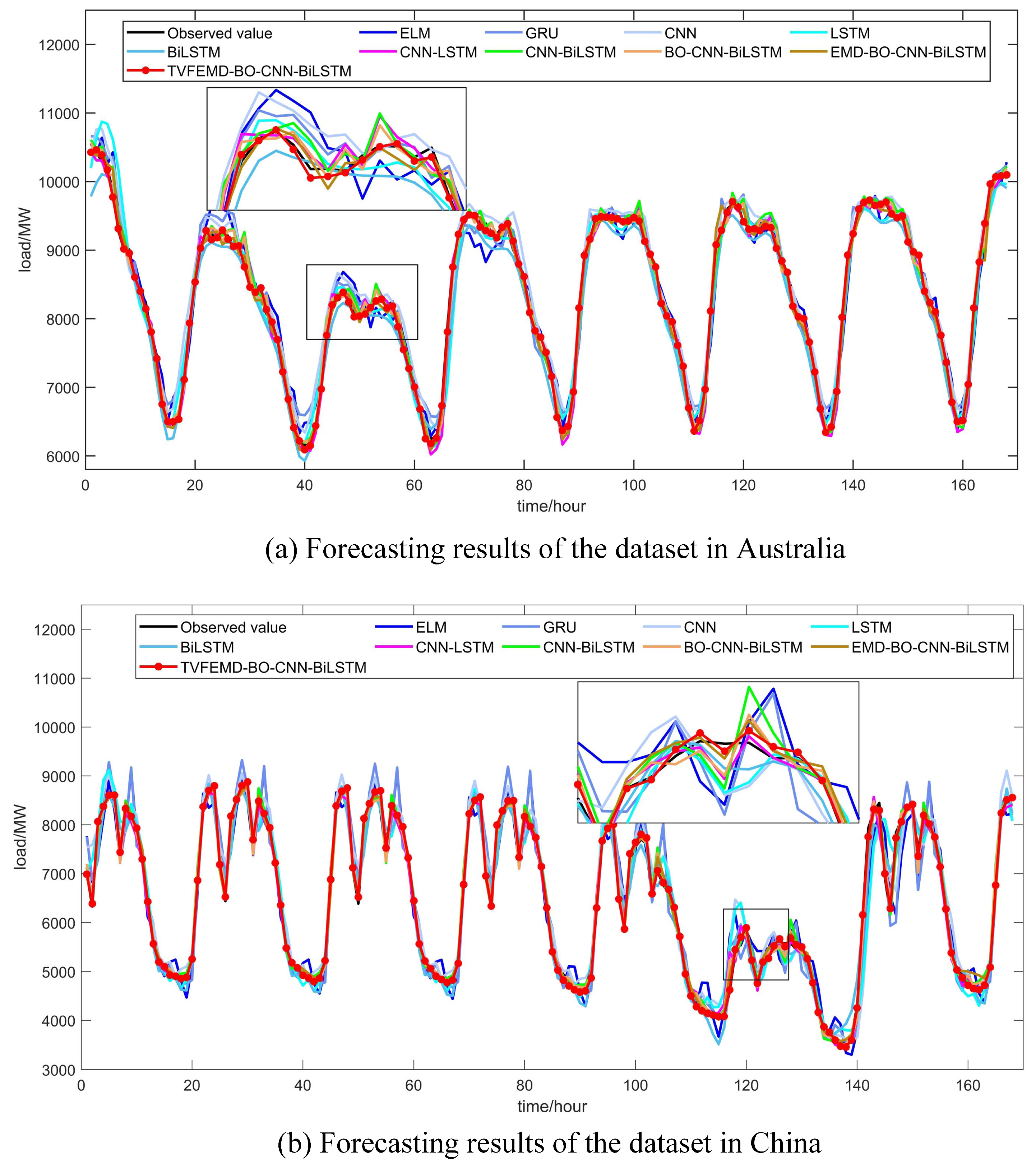
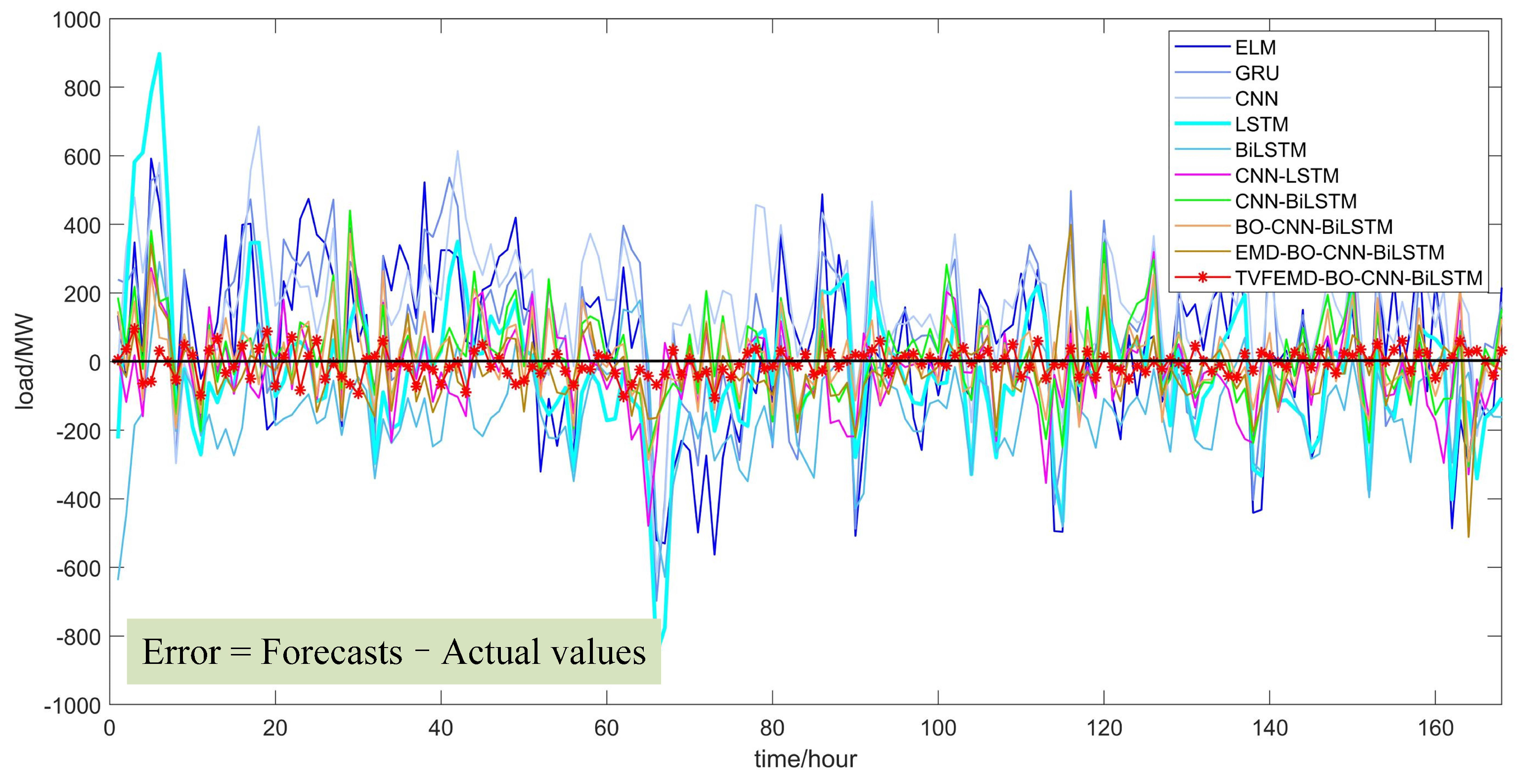
4.3. Experiment I: Online Feature Extraction Process Simulation

Datasets from Australia and China are applied to validate the performance of the TVFEMD-BO-CNN-BiLSTM model. The comparison models are divided into two types of predictive models. One type includes individual models, such as ELM, CNN, GRU, LSTM, and BiLSTM. The other type includes hybrid models, such as CNN-LSTM, CNN-BiLSTM, BO-CNN-BiLSTM, and EMD-BO-CNN-BiLSTM.
TVFEMD is used to decompose the historical power load sequence into multiple sub-series with different frequency division features. To improve the decomposition efficiency of TVFEMD, the left parts in Figure 2a,b show the decomposition results from the high-frequency series to the low-frequency series for Datasets 1 and 2, respectively. In this figure, the lines in order from top to bottom are the decomposition sequences  F 1 1 , F 2 1 , , F 10 1  and  F 1 2 , F 2 2 , , F 10 2 . It can be seen that the original power load sequences in Australia and China are divided into ten sub-series, which reflect the fluctuation pattern and local characteristics of the power load on different time scales.
A large number of sub-series may substantially increase the model’s forecasting time and computational cost. Hence, SE is used to conduct complexity evaluations for each sequence, and the evaluation results of each sequence are shown in Table 1. The series with similar frequency-division features are combined into a new sequence according to the sample entropy values. Series in Australia are reconstructed into five sub-sequences  S 1 1 , S 2 1 , S 3 1 , S 4 1 , S 5 1 , which are represented sequentially from the first line to the last line in the right part of Figure 2a. Meanwhile, series in China are reconstructed into six sub-sequences  S 1 2 , S 2 2 , S 3 2 , S 4 2 , S 5 2 , S 6 2 , expressed as in the right part of Figure 2b in order from the first line to the last line.
In this study, the hyperparameters of the proposed model are optimized using the Bayesian optimization algorithm, the results of which have been listed in Table 2. Additionally, to validate the effectiveness and generalization ability of the proposed model, we conducted experiments using two datasets with different features. The load forecasting results of ten models for a future week in Australia and China are shown in Figure 3a,b, respectively, which demonstrate the following conclusions: (a) Compared to the forecasting curves of other models, the forecasting curve of the proposed TVFEMD-BO-CNN-BiLSTM model is most closely aligned with the fluctuations in the actual power load curve, which means that the proposed model can better fit the trend of the actual power load, especially at the peaks and troughs of the curve. (b) The forecasting curves of the single models, such as ELM, CNN, GRU, LSTM, and BiLSTM, are consistent with the trend in the actual power load curve. However, in comparison to combined models such as CNN-LSTM and CNN-BiLSTM, the performance of single models is ineffective; the power load fluctuates substantially, such as in the curve’s peaks and valleys. Furthermore, four indicators, including MAPE, RMSE, MAE, and R2, are selected to quantify the error of the forecasting models.
To evaluate the prediction effect of each model more intuitively, the gap between the prediction results and the actual values under different datasets in Australia and China was calculated, and then the difference results were plotted as a curve, which is shown in Figure 4. The closer the results are to the horizontal line 0, the smaller the gap between the predicted values and actual values is and the better the prediction effect of the model. As can be seen from Figure 4, compared to other models, the error values at the red point in the curve of the TVFEMD-BO-CNN-BiLSTM model are closer to the horizontal line 0, which means that the proposed model better fits the fluctuation of the actual load values. Moreover, detailed error values are listed in Table 3.
From Table 3, it can be observed that the proposed TVFEMD-BO-CNN-BiLSTM model has the best forecasting performance, with the minimum MAPE, RMSE, MAE, and maximum  R 2 . Compared with the other nine models on the Australian dataset, the MAPE values of the proposed model are reduced by 1.9811%, 1.9669%, 1.9067%, 1.4504%, 1.5227%, 0.8999%, 0.8369%, 0.7279%, and 0.5089%, respectively; the RMSE values of the proposed model are lowered to 200.1098, 195.3382, 188.5207, 176.7032, 160.3596, 95.4436, 91.1594, 76.1276, and 60.5369, respectively; the MAE values of the proposed model are decreased by 161.3380, 156.6248, 154.3188, 120.7236, 128.9993, 72.7290, 70.9278, 61.4450, and 42.4828, respectively; and the  R 2  reaches 0.9988, which is the best result of all these models.
Due to the addition of the CNN local feature extraction module, the combination models are superior to individual models under different metrics for forecasting non-smooth time-series data. Additionally, the CNN-BiLSTM-based model has a better forecasting performance in capturing the long-term time-series characteristics of power load data.
Compared with the CNN-BiLSTM model, the MAPE, RMSE, and MAE are smaller and the  R 2  is larger in the BO-CNN-BiLSTM model, which indicates that BO can optimize the model hyperparameters to further improve the forecasting accuracy. EMD-based and TVFEMD-based models have lower forecasting errors than other forecasting models, which implies that the signal decomposition technique can deal with the noise in raw power load data effectively. Therefore, modal decomposition techniques can improve the forecasting accuracy. In addition, the decomposition effect of TVFEMD is better than that of EMD.

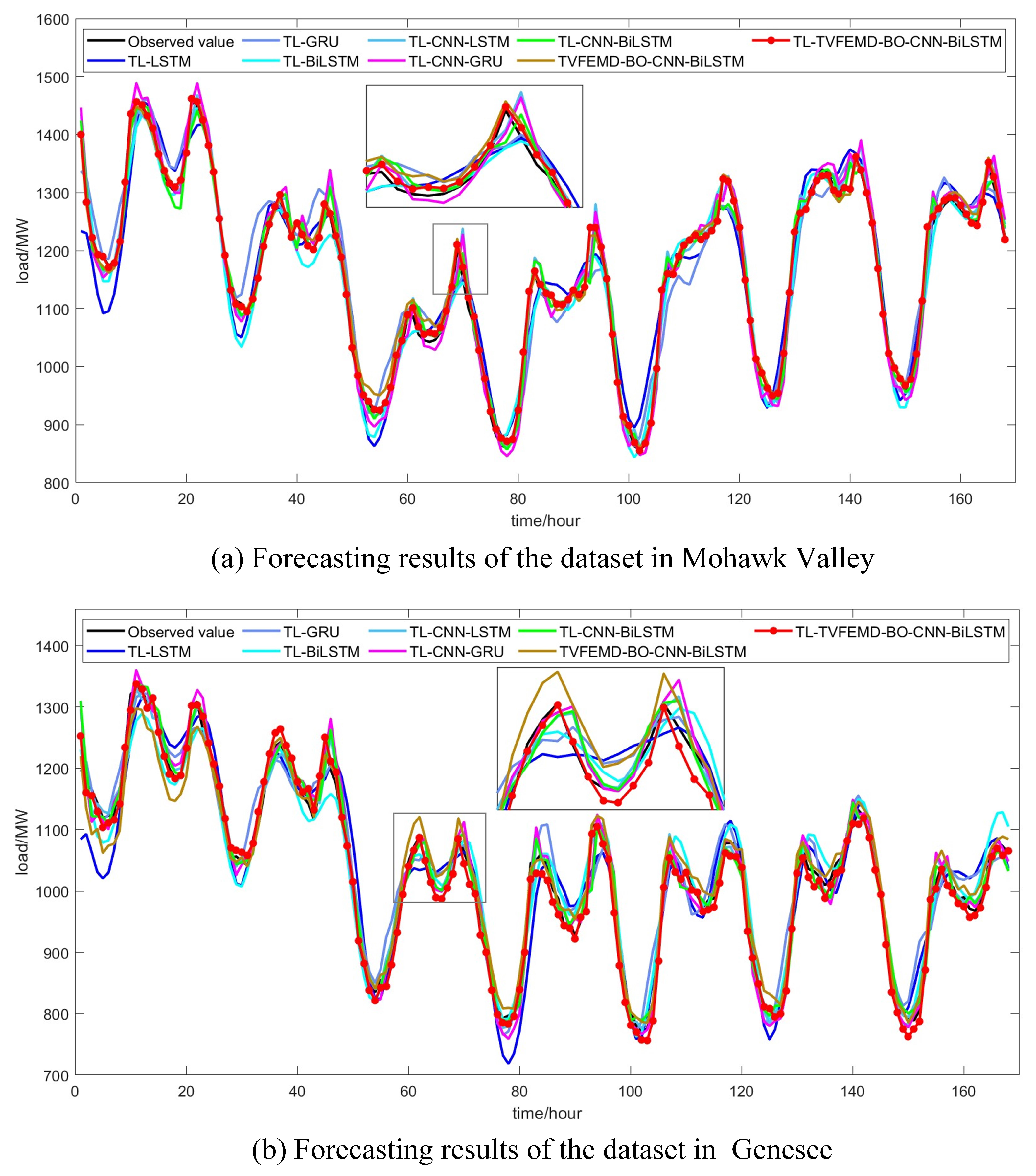
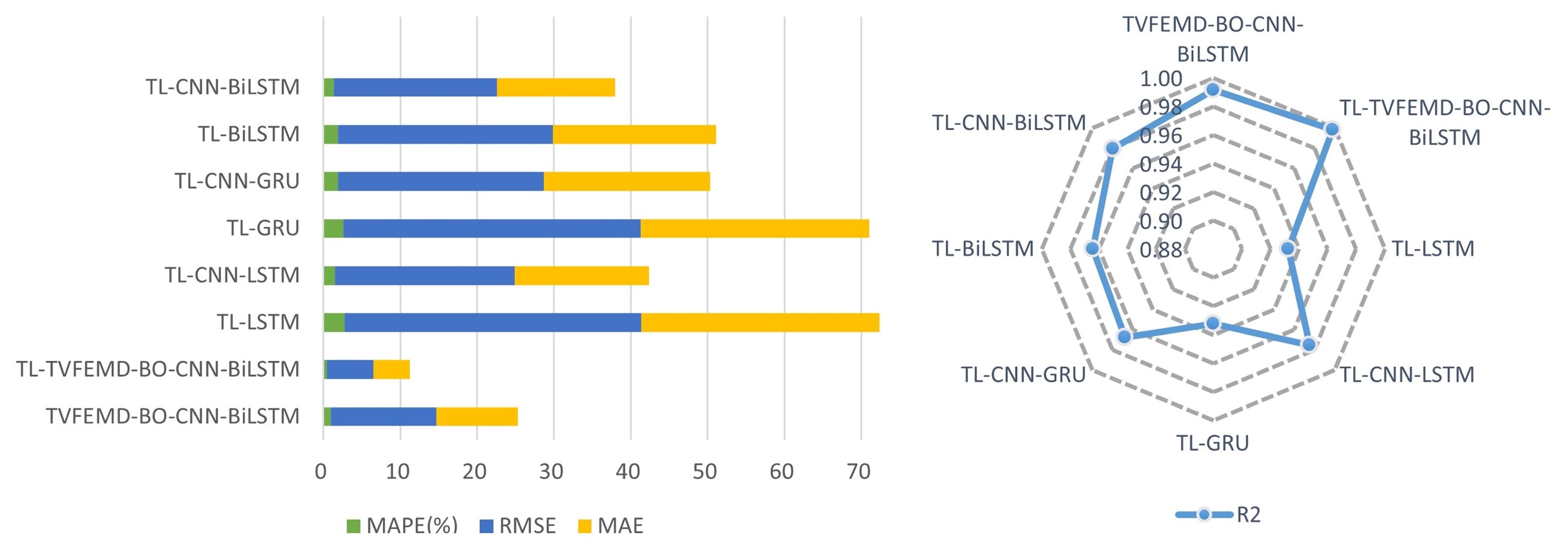
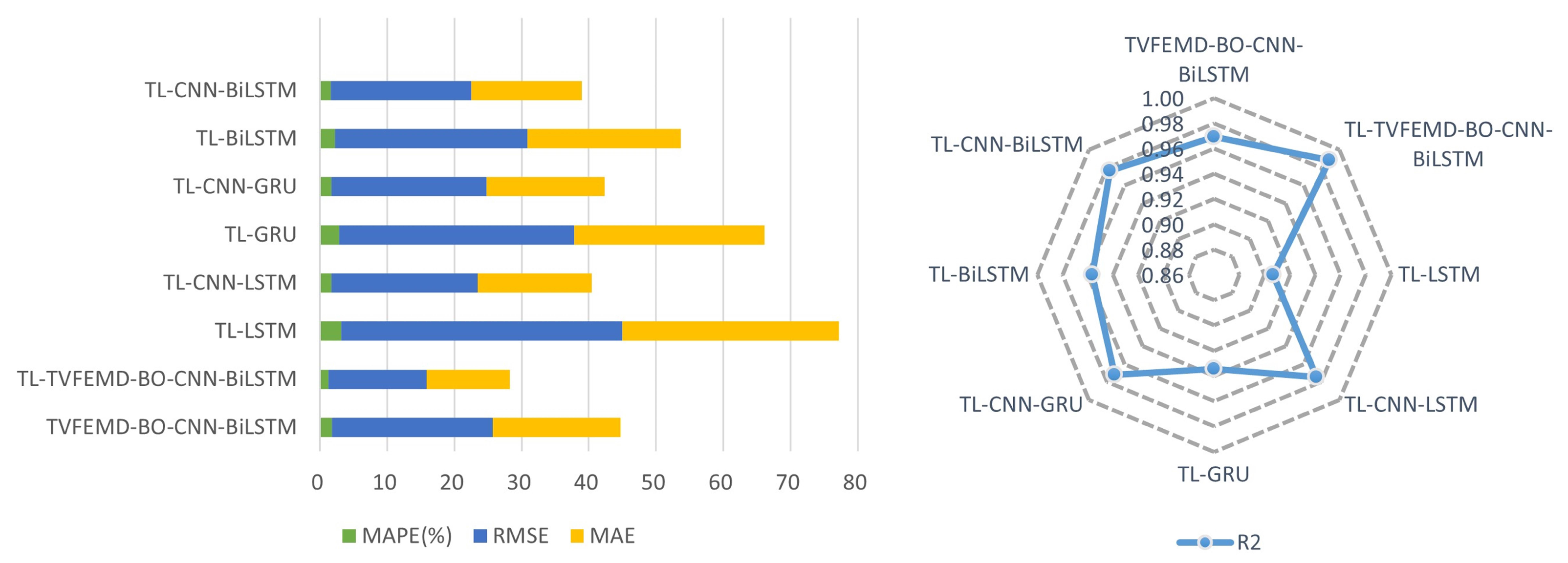
4.4. Experiment II: Transfer Learning Process Simulation

To verify the performance of the proposed model on the limited dataset, this study develops comparative models based on transfer learning (TL), including TL-LSTM, TL-GRU, TL-BiLSTM, TL-CNN-LSTM, TL-CNN-GRU, and TL-CNN-BiLSTM. In detail, the structure and weights of the input and hidden layers learned in the source domain are frozen and transferred to the target domain. Additionally, a TVFEMD-BO-CNN-BiLSTM model based on raw data is constructed to illustrate that the migration effect is positive. The hyperparameters of all these models are fine-tuned via the Bayesian optimization algorithm, which enables an efficient search for the best combination of hyperparameters.
In this study, the Kendall coefficient will be employed to calculate the correlation between the source and target domains, and the results are shown in Figure 5. As seen in Figure 5, the highest significant correlation, with a correlation coefficient of 0.8414, is between Central New York and the Mohawk Valley. The correlation coefficient between Central New York and Genesee is likewise significant, at 0.8399. Therefore, to ensure the credibility and representation of the experimental results, the hourly power load dataset in Central New York is utilized as the source domain and migrated to the target domains, including Mohawk Valley and Genesee, respectively. It is assumed that the target domain only has a power load from 1 to 31 January. We forecasted the power load for the week of 1 to 7 February using the proposed method based on transfer learning.
Figure 6a,b show a comparison of the forecasting results of the eight models after migration in Mohawk Valley and Genesee. The contours of power load profiles forecasted by each model are consistent with the actual power load, but there are still differences in the magnitude of the errors. Compared with other models, the forecasting performance of TL-LSTM is relatively poor, while the forecasting curve of the TL-TVFEMD-BO-CNN-BiLSTM model can fit the actual power load better. The forecasting errors of these models for the future week’s load can be seen visually in Figure 7 and Figure 8, and detailed error results are shown in Table 4.
In the left part of Figure 7 and Figure 8, it is intuitively observed that the bars for the MAPE, RMSE, and MAE in the TL-TVFEMD-BO-CNN-BiLSTM model are the shortest among all models. The R2 value of the model is closest to the boundary line with 1 in the radar plot. As presented in Table 4, regarding the coming week’s load forecast in Mohawk Valley and Genesee, the TL-TVFEMD-BO-CNN-BiLSTM model has a superior forecasting performance over other comparative models. For example, in comparison to other models based on transfer learning, for load forecasting in Mohawk Valley, the MAPE value of the TL-TVFEMD-BO-CNN-BiLSTM model decreases by 2.2936%, 2.1573%, 1.4415%, 1.0789%, 1.4510%, and 0.8964%, respectively; the RMSE value of the TL-TVFEMD-BO-CNN-BiLSTM model decreases by 32.5346, 32.5522, 21.8817, 17.2464, 20.6845, and 15.1349, respectively; yjr MAE value of the TL-TVFEMD-BO-CNN-BiLSTM model decreases by 26.2631, 25.0583, 16.5619, 12.7903, 16.9332, and 10.6666, respectively; and the goodness-of-fit coefficient R2 is as high as 0.9983. Furthermore, compared to pre-migration, the MAPE, RMSE, and MAE values in the TL-TVFEMD-BO-CNN-BiLSTM model are reduced by 0.5202%, 7.6002, and 5.8849, and the R2 is higher, which demonstrates that transfer learning can improve the accuracy of the forecasting model when dealing with a limited dataset.
By accurately predicting the future power load, the model proposed in this paper helps grid operators to rationally arrange the generation resources to avoid energy waste and cost increases, and also helps power companies to develop scientific operation planning to ensure the operation efficiency and stability of their power system. Moreover, the model based on transfer learning can be updated quickly to adapt to new data features, reducing the retraining time and costs.

5. Discussion

When implementing grid planning for low-carbon development, the feed-in power is dominated by a high proportion of renewable energy consumption. Nonetheless, increased output volatility from renewable sources causes increased power load volatility and intermittency. As a result, short-term electricity load forecasts face significant challenges and there are limitations in the implementation process, including data preprocessing, online feature extraction, model prediction costs, dynamic selection of hyperparameters, and hybrid model selection. In this study, the above problems are addressed using a hybrid forecasting model built by introducing a data-driven approach, artificial neural networks, and intelligent optimization algorithms. Forecasting results from the model provide decision-making information for new energy grid integration, such as layout planning, operational testing and management, scheduling and operational control, and access planning and management in new energy power generation equipment. Therefore, accurate power load forecasting results can mitigate the operational risks of the power system and resource waste such as power abandonment.
The electricity generated from renewable energy sources is affected by climate change, geographic location, and other factors, leading to large fluctuations in the time-series curve. If a prediction model directly performs a forecasting task, it experiences difficulty in recognizing the load’s characteristics, causing large prediction errors. Therefore, it is especially necessary to preprocess the data using a robust time-varying filtering-based EMD method, which can extract the load’s frequency-division characteristics at different times, allowing the prediction model to recognize and learn the load regularity. In this paper, the corresponding prediction model is constructed separately for each decomposed sequence and the Bayesian optimization algorithm is used to adjust the hyperparameters for sequences with different features to improve the prediction accuracy. To avoid excessive computational overhead due to over-decomposition, sample entropy is used to assess the complexity of the sequence and improve the model’s predictive efficiency.
The amount of effective and abundant power load data significantly affects the accuracy of the forecasting model. Scarce historical data may lead to a reduced forecasting accuracy, difficulties in power system risk management, inadequate energy planning, and increased operating costs. Real-life situations are often characterized by the scarcity of load data. For example, in areas where wind and solar energy is growing rapidly, it is difficult to predict the capacity of these energy sources due to poor stability and predictability, leading to a scarcity of electricity load data. Insufficient data for power load forecasting may also occur due to buildings lacking data collection systems, due to sensor malfunctions generating low-quality data, or due to newly constructed buildings coming online. In addition, collecting sufficient electrical load data is time-consuming and costly, and this may even make it difficult to meet quality requirements. Therefore, in the case of limited load data, there is a necessity to find an effective way to obtain enough high-quality data to train the model and improve the accuracy of the prediction model. In this study, transfer learning is introduced to solve this problem. We achieve the desired prediction accuracy with a limited dataset.

6. Conclusions

This study developed a hybrid method that not only dynamically extracts features from power load data but also reduces redundant learning of similar features. Additionally, this method is effective for limited datasets. The proposed model is verified on two different datasets. The specific conclusions are shown below:
(1) Compared with other models, the proposed model performs better in terms of the metrics of MAPE, MAE, and RMSE. The  R 2  values indicate that the proposed model has the best performance among all models and that it has a better forecasting performance and a stronger generalization ability on different datasets. Different experiments are conducted to verify the three modules of the proposed model, namely the feature extraction module, the hyperparameter optimization module, and the forecasting module. Reasonable comparison models are constructed to imply that each module can improve the forecasting accuracy.
(2) Decomposition and reorganization of temporal features can further mine potential information at different frequencies. The decomposition and reorganization process highlights that the power load shows certain fluctuation patterns on different time scales. In detail, the decomposed features are a series of different frequency bands, which are beneficial for feature recognition. The coalesced features ensure that the training process for the deep learning models is low-cost; furthermore, it can help in learning the frequency division of time series efficiently.
(3) The proposed hybrid model shows excellent performance on a limited dataset. In this study, transferability between different datasets has been measured to avoid negative transfer; the pretrained model is transferred to forecast power load data with a high similarity. In this way, the proposed model can achieve the desired forecasting accuracy without a large amount of training data.
The prediction method proposed in this paper is experimentally simulated on the public power load dataset and achieves an ideal prediction accuracy. However, there are still some deficiencies. Since actual grid data are confidential and difficult to obtain, the model in this paper was trained using early public datasets. Also, the model needs to be constantly revised using real-time data in practical applications. Therefore, in future research, the results of this paper will be applied to power load forecasting in a power system after a new energy grid is connected, not only to further validate the results of this paper, but also to enhance their application value. In addition, due to the black-box characteristics of deep learning models, it is difficult to explain and verify the prediction results of the models, which may lead to potential biases and errors in the models that are difficult to detect. Future research should explore ways to improve the interpretability of deep learning to make it more reliable and transparent.

Author Contributions

L.X.: Original draft preparation and editing; R.A.: Conceptualization and data collection; X.Z.: Writing and software. All authors have read and agreed to the published version of the manuscript.

Funding

This work was supported by the National Natural Science Foundation of China (No. 71901045); Science and Technology Innovation Project of The Chongqing Municipal Education Committee (No. KJQN202100604).

Data Availability Statement

Data cannot be released due to privacy.

Conflicts of Interest

The authors declare no conflict of interest.

References

  1. Guo, X.; Chen, L.; Wang, J.; Liao, L. The impact of disposability characteristics on carbon efficiency from a potential emissions reduction perspective. J. Clean. Prod. 2023, 408, 137180. [Google Scholar] [CrossRef]
  2. Asanov, M.; Asanova, S.; Safaraliev, M.; Zicmane, I.; Beryozkina, S.; Suerkulov, S. Design methodology of intelligent autonomous distributed hybrid power complexes with renewable energy sources. Int. J. Hydrogen Energy 2023, 48, 31468–31478. [Google Scholar] [CrossRef]
  3. Pawar, P.; TarunKumar, M.; Vittal K., P. An IoT based Intelligent Smart Energy Management System with accurate forecasting and load strategy for renewable generation. Measurement 2020, 152, 107187. [Google Scholar] [CrossRef]
  4. Vardhan, B.S.; Khedkar, M.; Srivastava, I.; Patro, S.K. Impact of integrated classifier—Regression mapped short term load forecasting on power system management in a grid connected multi energy systems. Electr. Power Syst. Res. 2024, 230, 110222. [Google Scholar] [CrossRef]
  5. Telle, J.S.; Upadhaya, A.; Schönfeldt, P.; Steens, T.; Hanke, B.; von Maydell, K. Probabilistic net load forecasting framework for application in distributed integrated renewable energy systems. Energy Rep. 2024, 11, 2535–2553. [Google Scholar] [CrossRef]
  6. Pramanik, A.S.; Sepasi, S.; Nguyen, T.L.; Roose, L. An ensemble-based approach for short-term load forecasting for buildings with high proportion of renewable energy sources. Energy Build. 2024, 308, 113996. [Google Scholar] [CrossRef]
  7. Wei, G.; He, J.; Zhang, Y. Application of the Unascertained Number in the Improvement of the Regressive Load Forecasting Model. High Volt. Eng. 2005, 31, 73–75. [Google Scholar]
  8. Smyl, S. A hybrid method of exponential smoothing and recurrent neural networks for time series forecasting. Int. J. Forecast. 2020, 36, 75–85. [Google Scholar] [CrossRef]
  9. Liu, Y.; Han, M.; Guo, J.; Liangli, S.U. Short-term electric load forecasting based on DBSCAN-ARIMA method. J. Beijing Inf. Sci. Technol. Univ. 2019, 34, 84–87. [Google Scholar]
  10. Tang, T.; Jiang, W.; Zhang, H.; Nie, J.; Xiong, Z.; Wu, X.; Feng, W. GM(1,1) based improved seasonal index model for monthly electricity consumption forecasting. Energy 2022, 252, 124041. [Google Scholar] [CrossRef]
  11. Chen, Y.; Xiao, C.; Yang, S.; Yang, Y.; Wang, W. Research on long term power load grey combination forecasting based on fuzzy support vector machine. Comput. Electr. Eng. 2024, 116, 109205. [Google Scholar] [CrossRef]
  12. Loizidis, S.; Kyprianou, A.; Georghiou, G.E. Electricity market price forecasting using ELM and Bootstrap analysis: A case study of the German and Finnish Day-Ahead markets. Appl. Energy 2024, 363, 123058. [Google Scholar] [CrossRef]
  13. Zhu, J.; Yang, Z.; Guo, Y.; Yu, K.; Zhang, J.; Mu, X. Deep Learning Applications in Power System Load Forecasting: A Survey. J. Zhengzhou Univ. Eng. Sci. 2022, 31, 3. [Google Scholar]
  14. Zhu, L.; Xun, Z.; Wang, Y.; Cui, Q.; Chen, Y.; Lou, J. Short-term Power Load Forecasting Based on CNN-BiLSTM. Power Syst. Technol. 2021, 45, 4532–4539. [Google Scholar]
  15. Wan, A.; Chang, Q.; AL-Bukhaiti, K.; He, J. Short-term power load forecasting for combined heat and power using CNN-LSTM enhanced by attention mechanism. Energy 2023, 282, 128274. [Google Scholar] [CrossRef]
  16. Michael, N.E.; Bansal, R.C.; Ismail, A.A.A.; Elnady, A.; Hasan, S. A cohesive structure of Bi-directional long-short-term memory (BiLSTM) -GRU for predicting hourly solar radiation. Renew. Energy 2024, 222, 119943. [Google Scholar] [CrossRef]
  17. Shao, Z.; Zheng, Q.; Liu, C.; Gao, S.; Wang, G.; Chu, Y. A feature extraction- and ranking-based framework for electricity spot price forecasting using a hybrid deep neural network. Electr. Power Syst. Res. 2021, 200, 107453. [Google Scholar] [CrossRef]
  18. Mounir, N.; Ouadi, H.; Jrhilifa, I. Short-term electric load forecasting using an EMD-BI-LSTM approach for smart grid energy management system. Energy Build. 2023, 288, 113022. [Google Scholar] [CrossRef]
  19. Yue, W.; Liu, Q.; Ruan, Y.; Qian, F.; Meng, H. A prediction approach with mode decomposition-recombination technique for short-term load forecasting. Sustain. Cities Soc. 2022, 85, 104034. [Google Scholar] [CrossRef]
  20. Gao, X.; Guo, W.; Mei, C.; Sha, J.; Guo, Y.; Sun, H. Short-term wind power forecasting based on SSA-VMD-LSTM. Energy Rep. 2023, 9, 335–344. [Google Scholar] [CrossRef]
  21. Xiong, D.; Fu, W.; Wang, K.; Fang, P.; Chen, T.; Zou, F. A blended approach incorporating TVFEMD, PSR, NNCT-based multi-model fusion and hierarchy-based merged optimization algorithm for multi-step wind speed prediction. Energy Convers. Manag. 2021, 230, 113680. [Google Scholar] [CrossRef]
  22. Zhang, W.; He, Y.; Yang, S. A multi-step probability density prediction model based on gaussian approximation of quantiles for offshore wind power. Renew. Energy 2023, 202, 992–1011. [Google Scholar] [CrossRef]
  23. Ye, R.; Dai, Q. A novel transfer learning framework for time series forecasting. Knowl.-Based Syst. 2018, 156, 74–99. [Google Scholar] [CrossRef]
  24. Li, K.; Li, Z.; Huang, C.; Ai, Q. Online transfer learning-based residential demand response potential forecasting for load aggregator. Appl. Energy 2024, 358, 122631. [Google Scholar] [CrossRef]
  25. Wei, N.; Yin, C.; Yin, L.; Tan, J.; Liu, J.; Wang, S.; Qiao, W.; Zeng, F. Short-term load forecasting based on WM algorithm and transfer learning model. Appl. Energy 2024, 353, 122087. [Google Scholar] [CrossRef]
  26. Yuan, Y.; Chen, Z.; Wang, Z.; Sun, Y.; Chen, Y. Attention mechanism-based transfer learning model for day-ahead energy demand forecasting of shopping mall buildings. Energy 2023, 270, 126878. [Google Scholar] [CrossRef]
  27. Yang, Q.; Lin, Y.; Kuang, S.; Wang, D. A novel short-term load forecasting approach for data-poor areas based on K-MIFS-XGBoost and transfer-learning. Electr. Power Syst. Res. 2024, 229, 110151. [Google Scholar] [CrossRef]
  28. Li, H.; Li, Z.; Mo, W. A time varying filter approach for empirical mode decomposition. Signal Process. 2017, 138, 146–158. [Google Scholar] [CrossRef]
  29. Richman, J.S.; Randall, M.J. Physiological time-series analysis using approximate entropy and sample entropy. Am. J. Physiol. Heart Circ. Physiol. 2000, 278, H2039. [Google Scholar] [CrossRef]
  30. Rafi, S.H.; Nahid-Al-Masood; Deeba, S.R.; Hossain, E. A Short-Term Load Forecasting Method Using Integrated CNN and LSTM Network. IEEE Access 2021, 9, 32436–32448. [Google Scholar] [CrossRef]
  31. Michael, N.E.; Hasan, S.; Al-Durra, A.; Mishra, M. Short-term solar irradiance forecasting based on a novel Bayesian optimized deep Long Short-Term Memory neural network. Appl. Energy 2022, 324, 119727. [Google Scholar] [CrossRef]
  32. Zhang, X.Y.; Watkins, C.; Kuenzel, S. Multi-quantile recurrent neural network for feeder-level probabilistic energy disaggregation considering roof-top solar energy. Eng. Appl. Artif. Intell. 2022, 110, 104707. [Google Scholar] [CrossRef]
  33. Wang, J.; Wang, H.; Wang, H.; Zhang, Z. Short-term Power Load Prediction of Bidirectional LSTM with ISSA Optimization Attention Mechanism. Proc.-Csu-Epsa 2022, 34, 111–117. [Google Scholar]
  34. de Almeida, F.A.; Romao, E.L.; Gomes, G.F.; de Freitas Gomes, J.H.; de Paiva, A.P.; Miranda Filho, J.; Balestrassi, P.P. Combining machine learning techniques with Kappa–Kendall indexes for robust hard-cluster assessment in substation pattern recognition. Electr. Power Syst. Res. 2022, 206, 107778. [Google Scholar] [CrossRef]
Figure 1. Power load forecasting with the limited dataset based on parameter transfer.
Processes 12 00793 g001
Figure 2. Decomposition and reconstruction results based on the TVFEMD-SE algorithm.
Processes 12 00793 g002
Figure 3. Forecasting results of the datasets in experiment I.
Processes 12 00793 g003
Figure 4. Forecasting error values in experiment I.
Processes 12 00793 g004
Figure 5. Heat map of correlations among New York State divisions.
Processes 12 00793 g005
Figure 6. Forecasting results of different models after migration in experiment II.
Processes 12 00793 g006
Figure 7. Comparison of MAPE, RMSE, MAE and  R 2  results after migration in Mohawk Valley.
Processes 12 00793 g007
Figure 8. Comparison of MAPE, RMSE, MAE and  R 2  results after migration in Genesee.
Processes 12 00793 g008
Table 1. Sample entropy and reconstruction of each sequence.
Australian
Dataset
Series   F 1 1   F 2 1   F 3 1   F 4 1   F 5 1   F 6 1   F 7 1   F 8 1   F 9 1   F 10 1
Sample entropy0.07590.04140.03180.03070.01720.01580.01310.01070.00740.0061
Reconstruction   S 5 1   S 4 1   S 2 1   S 2 1   S 1 1   S 1 1   S 1 1   S 1 1   S 3 1   S 3 1
Chinese
Dataset
Series   F 1 2   F 2 2   F 3 2   F 4 2   F 5 2   F 6 2   F 7 2   F 8 2   F 9 2   F 10 2
Sample entropy0.25720.15750.14210.11030.09570.09270.09020.07110.06420.0517
Reconstruction   S 3 2   S 1 2   S 1 2   S 1 2   S 2 2   S 2 2   S 2 2   S 4 2   S 5 2   S 6 2
Table 2. Hyperparameter settings for the proposed model.
ModelHyperparameterRangeAustralian DatasetChinese Dataset
Optimization ResultsOptimization Results
CNNnumfilter[2, 256]5764
sizefilter[2, 4]32
Dropout[0.01, 1]0.02080.0122
BiLSTMMaxEpoch[50, 100]4216
InitialLearnRate[0.001, 0.01]0.00120.0016
LearnRateDropPeriod[1, 100]85
LearnRateDropFactor[0.1, 1]0.10100.1244
Table 3. Error comparison of different model forecasting results in Australia and China.
ModelsDataset in AustraliaDataset in China
MAPE (%)RMSEMAE   R 2 MAPE (%)RMSEMAE   R 2
ELM2.3704239.4930192.93090.95505.5325443.1403345.20880.9176
CNN2.3562234.7214188.21770.95684.9592436.0833320.79370.9202
GRU2.2960227.9039185.91170.95924.5806403.8322293.33290.9316
LSTM1.8397216.0864152.31650.96343.8580360.6637244.05180.9454
BiLSTM1.9120199.7428160.59220.96873.2272264.0626199.90380.9708
CNN-LSTM1.2892134.8267104.32190.98571.7995157.0683113.39240.9897
CNN-BiLSTM1.2262130.5426102.52070.98661.7793153.3386112.10610.9901
BO-CNN-BiLSTM1.1172115.510893.03790.98951.6267142.4330101.96950.9915
EMD-BO-CNN-BiLSTM0.898299.920174.07570.99221.149694.423670.01630.9963
TVFEMD-BO-CNN-BiLSTM0.389339.383231.59290.99880.828950.9694364.98640.9982
Table 4. Error comparison of different model forecasts after migration in Mohawk Valley and Genesee.
ModelsDataset in Mohawk ValleyDataset in Genesee
MAPE (%)RMSEMAE   R 2 MAPE (%)RMSEMAE   R 2
TL-LSTM2.712938.666330.96170.93233.150741.860032.18330.9066
TL-GRU2.576638.683929.75690.93232.837935.028528.24720.9346
TL-BiLSTM1.860828.013421.26050.96452.219528.608822.88570.9564
TL-CNN-LSTM1.498223.378117.48890.97531.649921.828716.9930.9746
TL-CNN-GRU1.870326.816221.63180.96741.720223.077517.57070.9716
TL-CNN-BiLSTM1.315721.266615.36520.97951.603920.930816.46960.9766
TVFEMD-BO-CNN-BiLSTM0.939513.731910.58350.99151.821323.937418.98420.9695
TL-TVFEMD-BO-CNN-BiLSTM0.41936.13174.69860.99831.225614.635412.42560.9886
Disclaimer/Publisher’s Note: The statements, opinions and data contained in all publications are solely those of the individual author(s) and contributor(s) and not of MDPI and/or the editor(s). MDPI and/or the editor(s) disclaim responsibility for any injury to people or property resulting from any ideas, methods, instructions or products referred to in the content.

