Abstract
In Romania, natural gas production is concentrated in two large producers, OMV Petrom and Romgaz. However, there are also smaller companies in the natural gas production area. In these companies, the deposits are mostly mature, or new deposits have low production capacity. Thus, the production forecast is very important for the continued existence of these companies. The model is based on the pressure variation in the gas reservoir, and the exponential model with production decline is currently used by gas and oil producers. Following the variation in the production of the gas wells, we found that in many cases, the Gaussian and Hubbert forecast models are more suitable for simulating the production pattern of gas wells. The models used to belong to the category of poorly conditioned models, with little data, usually called gray models. Papers published in this category are based on data collected over a period of time and provide a forecast of the model for the next period. The mathematical method can lead to a very good approximation of the known data, as well as short-term forecasting in the continuation of the time interval, for which we have these data. The neural network method requires more data for the network learning stage. Increasing the number of known variables is conducive to a successful model. Often, we do not have this data, or obtaining it is expensive and uneconomical for short periods of possible exploitation. The network model sometimes captures a fairly local pattern and changing conditions require the model to be remade. The model is not valid for a large category of gas wells. The Hubbert and Gauss models used in the article have a more comprehensive character, including a wide category of gas wells whose behavior as evolutionary stages is similar. The model is adapted according to practical observations by reducing the production growth period; the layout is asymmetric around the production peak; and the production range is reduced. Thus, an attempt is made to replace the exponential model with the Hubbert and Gauss models, which were found to be in good agreement with the production values. These models were completed using the Monte Carlo method and matrix of risk evaluation. A better appreciation of monthly production, which is an important aspect of supply contracts, and cumulative production, which is important for evaluating the utility of the investment, is ensured. In addition, we can determine the risk associated with the realization of production at a certain moment of exploitation, generating a complete picture of the forecast over the entire operating interval. A comparison with production results on a case study confirms the benefits of the forecasting procedure used.
1. Introduction
In the context of a continuously growing global demand for energy sources, the efficient management of natural resources becomes crucial for society as a whole. The natural gas industry in particular faces complex challenges in forecasting and optimizing production at gas wells. In this sense, it is necessary to develop and implement advanced forecasting methods to ensure sustainable and efficient natural gas extraction [1,2]. Oil and gas reserve prediction methods include analogy, volume, material balance, production decline, extrapolation, and gray system methods [3].
The ways of making production forecasts at natural gas wells emphasize distinct models: the exponential model, the Gaussian model, and the Hubbert model, or numerical reservoir simulation methods, the Weibull model, the Weng cycle model, and the HCZ model [4,5,6,7].
Hubbert’s basic petroleum resource depletion model, the Hubbert curve, became the foundation for a variety of curve-fitting techniques that are still widely used today. The strengths and weaknesses of these models were expressed in the current literature for determining their suitability for use in different situations [8,9,10,11].
Each of these approaches provides a unique perspective and specific methodologies for evaluating the production and forecasting future quantities of natural gas that can be extracted. The Hubbert model [12], originally developed for estimating oil production, has also been adapted for the natural gas industry. The model focuses on the concept of peak production and how it provides a long-term perspective on production evolution, contributing to the development of sustainable strategies for resource utilization.
However, studies have shown that the incorrect selection of initial values [13] can lead to poor modeling capacity and adaptability and to troubles in obtaining high-performance results. The Hubbert model has been improved and the results thus obtained are much more accurate for the prediction of natural gas reserves and consistent with the trend of increasing production and then maintaining production after commissioning [14,15].
In [16], a gray model is built for the prediction of tight gas production. The Gray Model Tight Gas Production (GMTGP) presented in this paper solves the problem of the reasonable prediction of tight gas production in China. The model is compared with other classic models of gray model theory: the GM(1,1) model, a univariate first-order derivative gray prediction model mainly used to study prediction problems of time-series data with homogeneous approximate exponential growth; GM(2,1) has a second-order derivative and two characteristic roots and can reflect the monotony situation or the oscillation of the theoretical system; GVM (Grey Verhulst Model) is mainly used to study the prediction problems of S-shaped sequences with saturation.
In [17], the reduction in the drilling cost of new wells is analyzed. One of these methods is the optimization of drilling parameters to establish the maximum available rate of penetration (ROP). There are many parameters that affect ROP. Therefore, developing a logical link between them to help in the correct selection of ROP is highly necessary and complicated. In such a case, artificial neural networks (ANNs) are proven to be useful in recognizing the complex connections between these variables. The ANNs could also be applied to the study of production forecasting problems.
The Hubbert and Gauss models are combined with Monte Carlo simulation, used to calculate the probability of production achievement. It is also used in the risk level assessment matrix of natural gas production [18]. These methods with promising results are also used in this article. The Monte Carlo method makes an important contribution in this sense by simulating multiple possible scenarios [19]. This technique generates a set of results based on random variables, reflecting the diversity of production conditions. By exploring these scenarios, a deeper understanding of potential risks and possible changes in production is obtained, providing essential information for strategic decisions [20,21]. In support of these models, a large collection of production data is continuously made. Modern data measurement, storage, and analysis tools are used [22,23,24].
The Gauss method is a mathematical approach that uses the normal distribution to estimate future natural gas production [25,26].
The Gauss model is better suited for predicting the growth pattern of natural gas reserves with gradual changes. This is because the peak time of the model is relatively late, and the curve tends to be wide and increases gradually at first, then rises rapidly, before increasing slowly and eventually reaching a peak and declining in a symmetrical form [27]. By modeling the normal distribution of key variables such as gas flow, this method accurately estimates the probabilities associated with each scenario, providing a more comprehensive view of possible fluctuations in production. This statistical approach provides a rigorous framework for evaluating production variability and anticipating unexpected events that may impact natural gas exploitation. There are also studies and models used to forecast the evolution trend of natural gas reserves using the multi-cycle Hubbert and Gauss models that give very good results [28,29].
The Hubbert and Gauss models can be used to assess the multi-cycle evolution of natural gas reserves, assuming that the parameter values are known and a mathematical forecasting method can be applied [30,31]. By combining the multi-peak Gauss model with the characteristics of reserves and production growth, some researchers were able to predict the growth trend of reserves and production by fitting historical curves [32].
Researchers have used various models to predict the proven reserves of natural gas. The Poisson model was used to show that the growth trend of proved natural gas reserves has a significant cyclical characteristic [33]. The improved Weng model and Weibull model were also applied, and the potential and exploration status of natural gas resources were analyzed [34]. Additionally, the HCZ model was used to predict the growth trend of proven natural gas reserves throughout the life cycle [35].
By analyzing and comparing these models, the article aims to provide a comprehensive perspective on the various approaches used in natural gas well production forecasting. Finally, we evaluated the advantages and limitations of each model, highlighting the importance of adaptability and the integration of multiple methods to obtain more accurate forecasts and useful information in the decision-making process in the natural gas industry.
For statistical forecasting models applied to production fields with a short interval of use, customization is required. In this article, the Hubbert and Gauss models were adapted according to practical observations by reducing the production growth period; the layout is asymmetric around the production peak; and the production range is reduced. These models were completed using the Monte Carlo method and a matrix of risk evaluation.
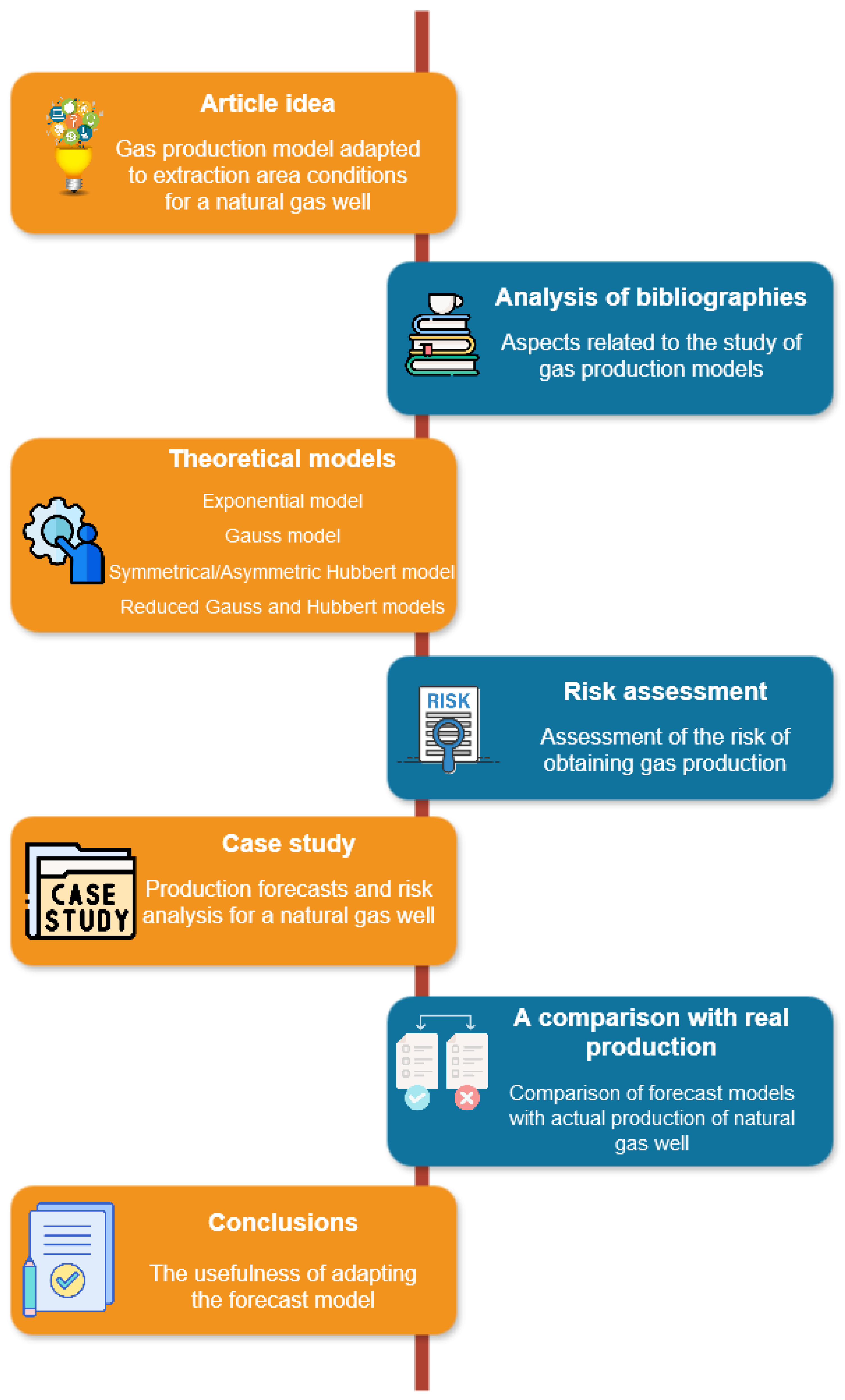
The steps of making the article are shown in Figure 1.
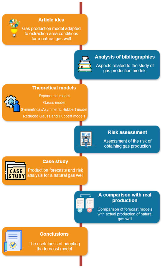
Figure 1.
The stages of making the article.
2. Theoretical Elements Related to Natural Gas Production Estimation Models
2.1. Production Models
The statistical examination of the authentic historical data of a huge number of gas field reservoirs helped many researchers to find and propose a series of natural gas reserve prediction models [22,29].
2.1.1. Exponential Model of the Production Variation
In this case, the production forecast for a gas well involves the following steps:
Collection of gas well information. Geological information is used on the structure where the positioning of the new gas well is planned. This information includes the type of new or matured field; reservoir limits; existing seismic data (3D seismic data require 3D seismic reinterpretation); and gas pressure and temperature at the reservoir level [23]. The difficulties that might arise during the execution of wells related to cementing operations are well route; disposition of productive layers; problems of unconsolidated layers and sand problems; and gas layers inter-bedded with thin water layers. To execute a new well, structural maps are used that are in the company’s database or the ANRM (National Agency for Mineral Resources of Romania) database and that contain information about productive, abandoned, and suspended wells; drilling difficulties; etc.
For a new gas well, proposed coordinates for its placement are suggested, and seismic investigations are conducted to substantiate the elements used in the forecast [34,35].
Selecting the possible production flow values. In general, knowing the exploitation history, the values of the minimum, average, and maximum hydrocarbon flows that can be obtained are anticipated. Usually, three forecast variants—High Estimation, Best Estimation, and Low Estimation—are elaborated.
These variants also assess the extracted condensate flow and the extracted water flow. Cumulative quantities of natural gas, condensate, and water are also evaluated.
The optimistic forecast High Estimation sets a high flow rate for gas and a correspondingly high cumulative production. The exploitation period of the well is longer. The Low Estimation variant reduces all of these values, ultimately resulting in lower cumulative production and a reduced gas well life. Comparing the extreme variants, High Estimation and Low Estimation, the former offers a lower probability of realization, while the latter has a higher probability of occurring. Therefore, we are either at a high risk or a low risk with the forecast.
The assumption of a gas flow rate variation law. The realization of the forecast starts from an initial value of the average gas flow that can be obtained daily . Relation (1) is used to express the evolution of this flow over time. The assessment is to decrease the average daily flow with a production decline factor , the law of variation being exponential; see Relation (1) [6,18].
where is the average daily gas flow achieved in the production month . The production time is measured in months. Logarithmizing Relation (1) shows that the variation in the logarithm of the average flow is linear concerning time. The slope of this line is the decline factor :
The decline factor is for gas exploitations of 0.04 . The monthly throughput is obtained by multiplying this relationship by the number of production days per month (3). The number of production days that is generally chosen identically for all months is equal to 29.5 ; see Relation (3). This takes into account possible production interruptions.
Cumulative production is calculated by summing the monthly productions. The production time (starting from month 1) is measured until a minimum gas flow is reached, beyond which the expenses for the well maintenance exceed the benefits obtained through selling the production, in month . The usual values of this minimum flow are between 5 and 12 (148–354 ).
The economic evaluation. Based on these assumptions, a final economic analysis is conducted for all three estimation variants (High Estimation, Best Estimation, and Low Estimation), which includes expenses related to well construction, production maintenance, and abandonment. Profits from the sale of production are assessed. These calculations are performed with the idea of an update of the values to take into account the influence of time on the expenses. The decision to dig the new gas well or to abandon the project is finally made.
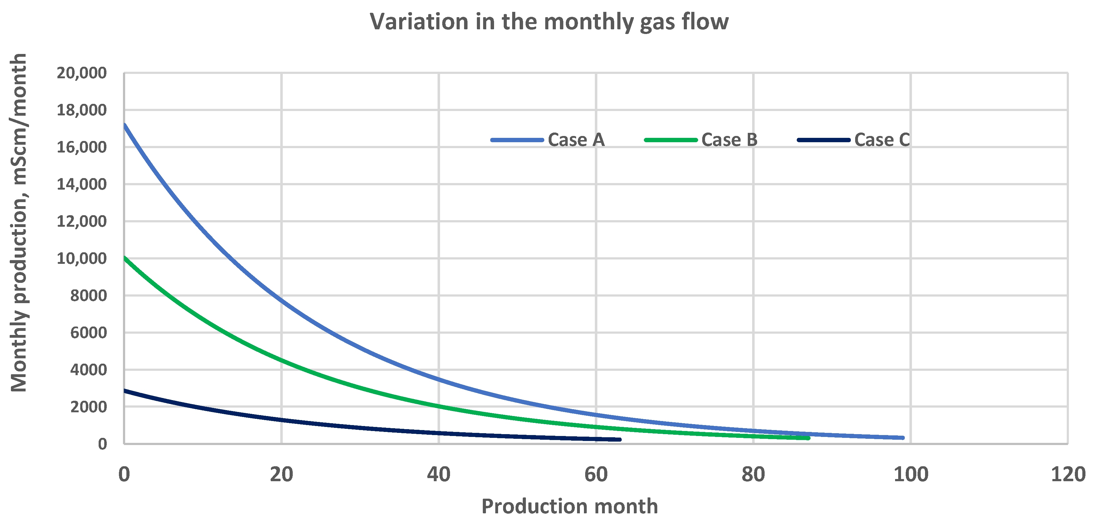
In Figure 2 and Table 1, the forecast for the three estimations based on initial flow rates and the minimum acceptable flow rate is observed (an example). The possible duration of production exploitation is determined from the cumulative production charts until reaching the economically minimum flow rate, as shown in Figure 2.
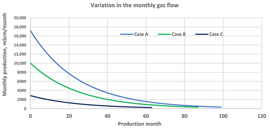
Figure 2.
The time variation model for the production of a gas well expressed in the monthly gas flow due to the decrease in the pressure in the reservoir (exponential model), for each of the three initial flow hypotheses (start/end flow values): case A—High Estimation (17,194/327 mScm/month), case B—Best Estimation (10,030/309 mScm/month), and case C—Low Estimation (2865/230 mScm/month).

Table 1.
The exponential production decline analysis model.
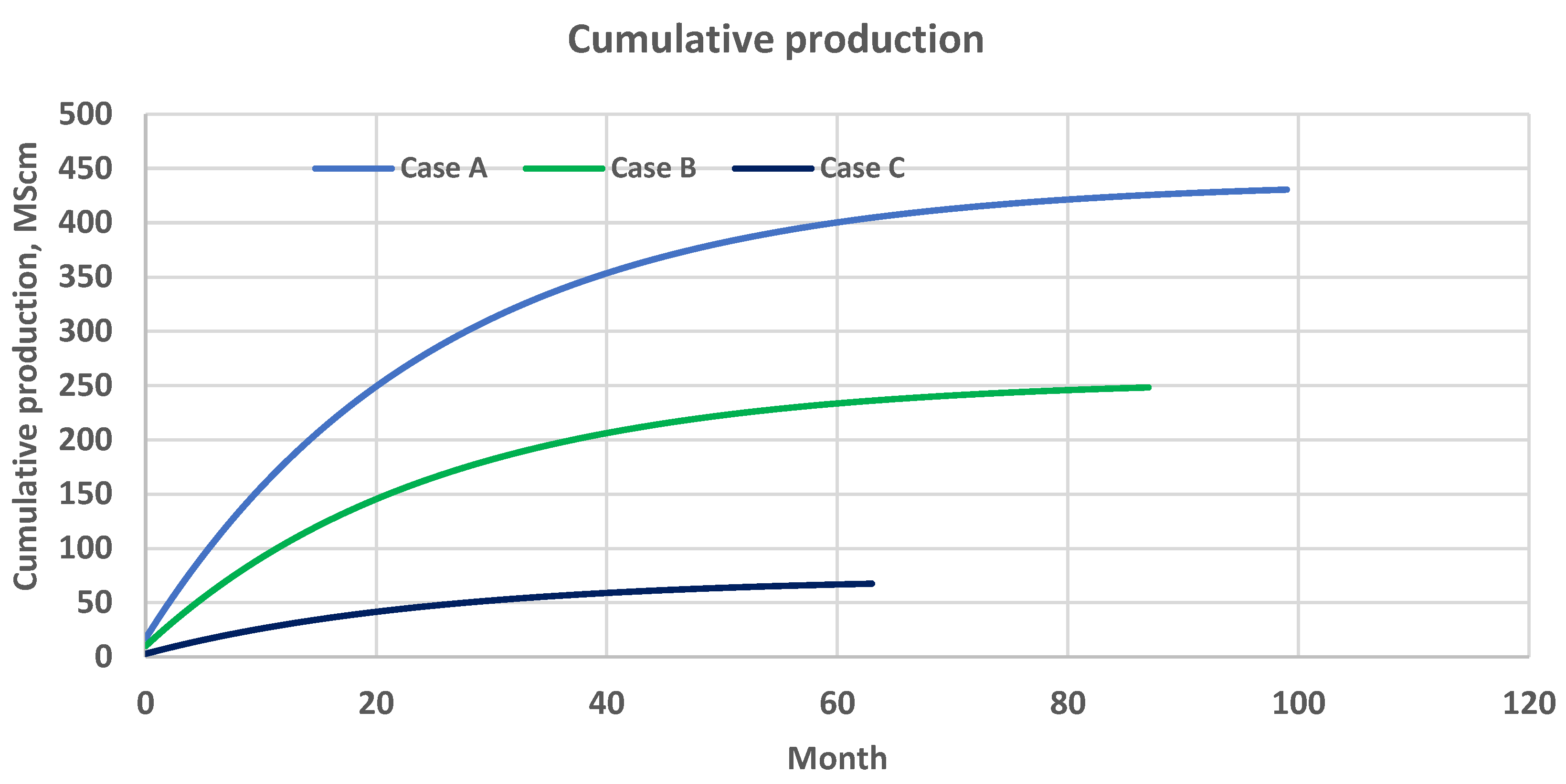
The cumulative production charts in Figure 3 show the maximum amount of gas that can be obtained by exploiting the respective deposit. The idea of the exponential model leads to a decreasing monthly production starting from a maximum value, a total volume of gas recoverable from the deposit, and a duration of exploitation of that deposit. However, taking into account the gas flow through the interstices, the supercritical flow regime provides a constant flow rate through these wells when the pressure drops until the critical threshold. These aspects can be seen in the form of production diagrams in some gas wells after a period of making circulation paths through the deposit. Thus, we have to give up on the exponential model in certain situations. The exponential model is much more suitable for crude oil wells.

Figure 3.
Cumulative production variation in the three cases of analysis of a gas well based on the exponential model (end flow values): case A—High Estimation (430.48 MScm), case B—Best Estimation (248.23 MScm), and case C—Low Estimation (67.44 MScm).
Commenting on Table 1, the optimistic forecast case starts from a flow of 17,194 and stops when the daily flow reaches the value of 327 . Included in this range is 99 months of production. The cumulative production is 430.48 .
The end flow value of the natural gas is an economic minimum value of the flow, shown in Figure 2. The cumulative production values are calculated for the number of months of production anticipated by the model.
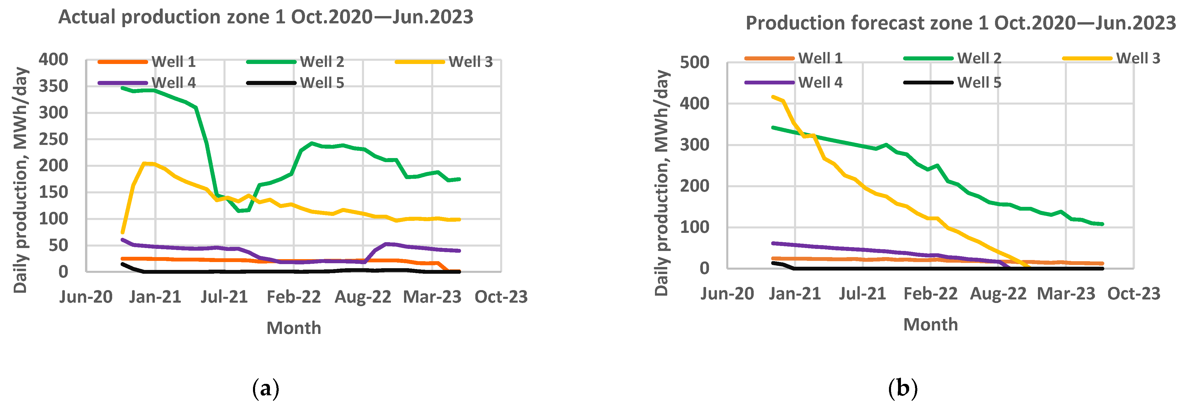
A production decline factor of 0.04 was considered. The assessments are similar for the other two situations, the Best Estimation and the Low Estimation. Some examples of variation in the predicted production are introduced (in the exponential model) compared to actual gas well production. It can be seen in Figure 4 that the forecast model is the one in Figure 4b (exponential) and this is achieved (from the point of view of the form of variation) in certain situations (gas wells 1 and 5) but sometimes presents both quantitative and qualitative differences (gas wells 2, 3, and 4).
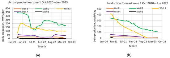
Figure 4.
Comparison of actual and anticipated production results: (a) actual production of five natural gas wells from zone 1; (b) production forecast of the natural gas wells from zone 1.
2.1.2. Hubbert Model
In the work on gas well production estimation, many approaches try to model these wells and assess the associated production stability risks. For these models [6,18], gas production decreases continuously from an initial value.
Although this model is not valid for all gas wells, it is used because it coincides with the behavior of many wells in the field (mostly oil wells). How communication occurs between different areas of the reservoir, the influence that gas flow has on communication possibilities within the deposit, the interaction with adjacent reservoir zones, the rock nature, and the extraction technology constitute many of the factors that are challenging to incorporate into a model [35,36].
The Hubbert model is often used to predict the production of natural gas wells. The model has the following features, according to [7,8,9,16]. After gas exploitation has been put into operation, production starts from zero, increases over time, and reaches its maximum value. Subsequently, there is the production decline phase, which can occur at a faster or slower pace. In the last phase of exploitation, the gas well has a production with a slow decrease, and after a while, the production stops; see Figure 5a.
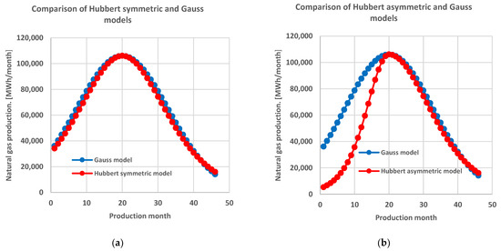
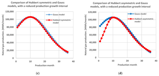
Figure 5.
Prediction of natural gas production: (a) symmetric Gauss and Hubbert models; (b) Gauss and asymmetric Hubbert models; (c) Gauss and symmetrical Hubbert models with a reduced production growth interval; (d) Gauss and asymmetric Hubbert models with a reduced production growth interval.
Next, the production decreases until the resources are depleted and the area under the graph of the variation of production over time is equal to the total volume of resources that can be obtained (expressed in standard cubic meters of gas or megawatt hours), according to [6,18]. Hubbert’s formula for cumulative production in this model is as follows:
where is the cumulative natural gas production; is the value of the recoverable resource from the deposit; means the time at which the production peak is reached; and is the slope corresponding to periods of increased or decreased production (in the Hubbert asymmetric model, the values are different).
By deriving Formula (4) concerning time, the expression of the monthly production (expressed in ) can be obtained:
This derives monthly production:
where is equal to , the maximum monthly production, which is given in the relation:
Formula (7) can be substituted in the expression number (5) and a simpler relationship is obtained for the production value using the Hubbert model [9,30]:
In Figure 5a,
Since the rising phase of a well’s production is faster than its declining phase, the asymmetric Hubbert model is suitable to suggest this aspect; in Figure 5b, . Although the Hubbert model is used for the exploitation of various resources, in natural gas wells, the production does not increase from zero to the maximum value and the first values obtained for a gas well are (initially) higher [16]. The rising phase of a gas well’s production is also shorter than its declining phase. Thus, it is preferred to eliminate a part of the left side within this model; values that are not obtained in practical situations. In Figure 5c, the following situation is represented for the Hubbert symmetric model: , and in Figure 5d for the Hubbert asymmetric model: .
2.1.3. Gauss Model
The Gauss model is similar to the Hubbert model and expresses the production value of a gas well [6,18,30,37]. The relation expressing the probability density for the Gaussian model is as follows:
where is the average value and is the standard deviation in the well exploitation process. The cumulative production in the interval [0,], considering the exploitation time , is denoted by . Multiplying the probability density function with the gives the relationship for the monthly natural gas production:
Taking the derivative of natural gas production concerning time and equating one to zero gives the maximum production at time .
Substituting this relationship into the monthly production yields the maximum production value:
Finally, the relationship of production can be arranged in the following form [18]:
Shown in Figure 5a,b, . In the same way as the Hubbert model, the area to the left of the maximum point for small production values was excluded so that the study could be conducted on a domain equal to 3 sigma (): 1 sigma () domain to the left of the maximum point and 2 sigma () domains to its right side; see Figure 5c,d, where
2.2. Theoretical Elements Related to the Evaluation of Production Risk
The Monte Carlo method is frequently used to emphasize the connection between a model of a physical system [19,37]. To use the method, the following steps are necessary: establishing the mathematical model for the target parameter, for example, the value of gas production; establishing the independent variables in the model; determining distribution functions for the independent variables; setting the number of simulations; determining the distribution function and the characteristic elements for the observed quantity.
In Equation (13), which expresses the value of production through the Gauss model, this method of production appreciation is used. There are three variables in the model: the maximum value of production; the time at which the maximum production value is obtained; and scattering the values of production times around the mean value. All these three variables have certain probability distribution functions. Considering the performance of modern programs, the number of tests can be greatly increased. Thus, the distribution function for the gas production value is estimated and the probability of obtaining a certain value is evaluated. These elements are useful during the early development of a well to anticipate possible performance during development.
For assessing the risk in production realization, an evaluation matrix is created based on two indicators: the first indicator is the probability of achieving the production and the second indicator is the degree of dispersion of the production. For the degree of dispersion of production, the following relationship is applied [18]:
Essentially, the risk matrix for a gas well expresses the probability of extracting gas from the discovered deposit and the duration of the exploitation of the well. These models, like the model used for production forecasts, have a degree of uncertainty and may fail in some situations. However, in their construction, a whole series of elements are used that are related to the deposit, the construction method of the gas well, and its exploitation, so that decisions are made based on better information. We cannot determine the probabilities of how long a well will last and the quantities of gas that can be extracted without using these models, which (hopefully) will become better and better.
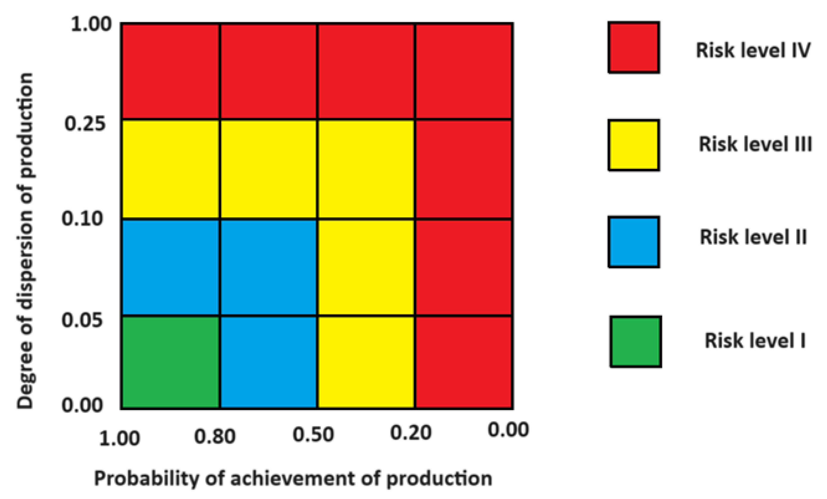
The risk matrix is represented in Figure 6 and structured on four levels [18]. Level I of risk is represented by the green color on the chart. In this situation, production can be conducted very easily. The criteria are the probability of achievement being and the spread level being . Level II of risk is represented by the blue color, where production is easy to achieve; the criteria used are the probability being and the dispersion of production being , or the probability of achieving production being and the degree of dispersion being . Level III of risk is represented by the yellow color. The production can be obtained when the probability of obtaining the production is and the dispersion is , or the probability of obtaining the production is and the dispersion is The risk of level IV is represented by the red color, where production is not easily achieved. The evaluation criteria are the probability of obtaining production being or the probability of obtaining production being and the dispersion being .
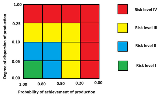
Figure 6.
Assessing the risk of achieving natural gas production using the risk matrix. The risk levels are in order from I to IV, with level I representing the lowest risk and level IV representing the highest risk.
Commenting on the relationship that provides the degree of dispersion of production, it can be observed that when there is a larger spread of production data, the value of dispersion approaches one, indicating a high risk. When the average value of the data is higher, then the degree of dispersion of the production is lower because the time interval in which the production is achievable is wider, which implies a greater period of the exploitation of the well. These arguments together with the probability of production realization are the basic elements that underlie the construction of the risk matrix [8,18,30]. It is useful for these aspects of assessment risk to be implemented in production analyses.
3. Case Study Analysis of the X Gas Well
3.1. Establishing the Gaussian Model of the Gas Well
To establish the Gaussian model of the gas extraction well, the following elements are known.
The gas capacity of the gas storage was determined through specific investigations [23,36]. Expressed in the energy unit MWh (or in a volume unit, Scm), this capacity is equal to 1.19 × 10⁷ MWh (1.21 × 10⁹ Scm), at a higher calorific value of the gases from the deposit of 9900 kWh/Scm (note that the previously shown example of the exponential model was applied to the same gas well).
An insight into the relationship between the gas volume estimated by measuring instruments and the proven gas volume in the region where these deposits are exploited is expressed by the factor The factor is included in of the estimated value. We can, therefore, anticipate a gas quantity between [5.97 × 10⁶ and 8.36 × 10⁶] MWh.
The recovery factor of the amount of gas for that area is estimated using the exploitation history at . Thus, the gas volume range that can be recovered is [4.12 × 10⁶; 5.77 × 10⁶] MWh.
In addition, we consider the effect of the technical conditions, including the ways of making the well hole and the possible problems that appear during exploitation as a factor that can decrease the amount of gas obtained [13]. We estimate the influence of this factor on the amount of gas to be equal to . Finally, the gas volume range that can be exploited is [2.88 × 10⁶; 4.04 × 10⁶] MWh. It is noted that within these assessments, we are quite prudent. If the production model provides higher values, it is all the better. There are many factors whose values are estimated. Thus, very large variations of the values appear, decreasing the quality of the estimate [16,36].
The history of gas production areas does not provide a long time for a particular production field. In general, the deposits available in Romania for small companies are mature deposits or deposits with reduced capacities. The large gas producers in Romania own most of the large fields where the exploitation period is much longer. Taking into account this observation, the discrete moments of analysis are in the order of months. In the example given for one of these companies with a small production capacity, which represents a small part of natural gas extraction in Romania, the possible duration of exploitation is between three to five years. We anticipated a production period of 39 months.
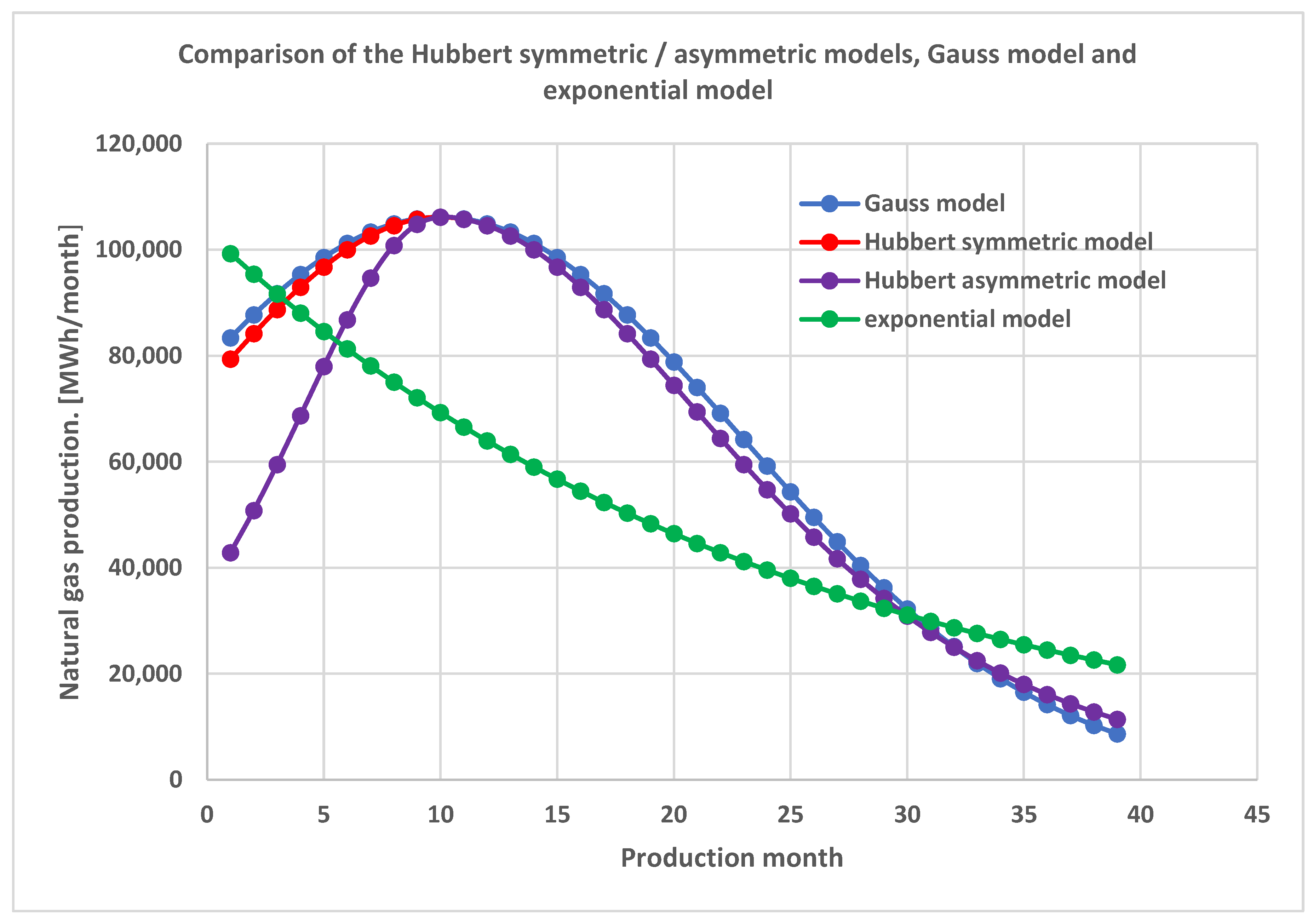
It is known that within the Gaussian model, 95% of the possible values are entered in the 4-sigma interval. As we stated when presenting the relations of the theoretical model, we used an interval equal to 3 sigma (positive values in that interval), because the initial production period does not have small values for gas production. Then, an acceptable value for the standard deviation is 13 months (39 months assumed to be in operation divided by 3). In the case of the model considered for this gas well, this standard deviation value was used in Relation (12). Using Relation (12), the maximum amount of gas that can be extracted monthly can be determined. It is included in the range [88,461; 123,846] . The time taken to achieve the production peak was 10 months from the start of the project Generally, after reaching a production maximum, this value is maintained for some time. This time point of the beginning of maximum production was chosen. With these considerations, Figure 7 shows the forecast made with the help of a program for the exponential model, the Gauss model, and the symmetric and asymmetric Hubbert model.
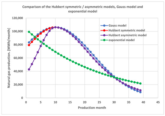
Figure 7.
The models used to make the production forecast at the analyzed gas well, ; ; (PNG, Production of Natural Gas).
The choice of Gauss/Hubbert models for this well was also suggested through the history of productions in the considered area, which departs from a decreasing pattern of production, as suggested using the exponential model. This history is represented in Figure 8, associated with wells in this production area.
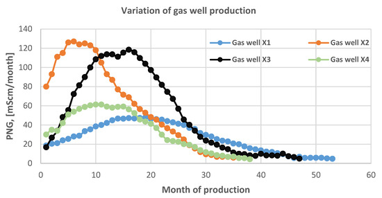
Figure 8.
Variation in the production at natural gas wells in the oil field of which the exemplified well is a part (PNG, Production of Natural Gas).
3.2. Results Regarding the Risk Analysis in the Case of the Forecast Made with the Gaussian Model
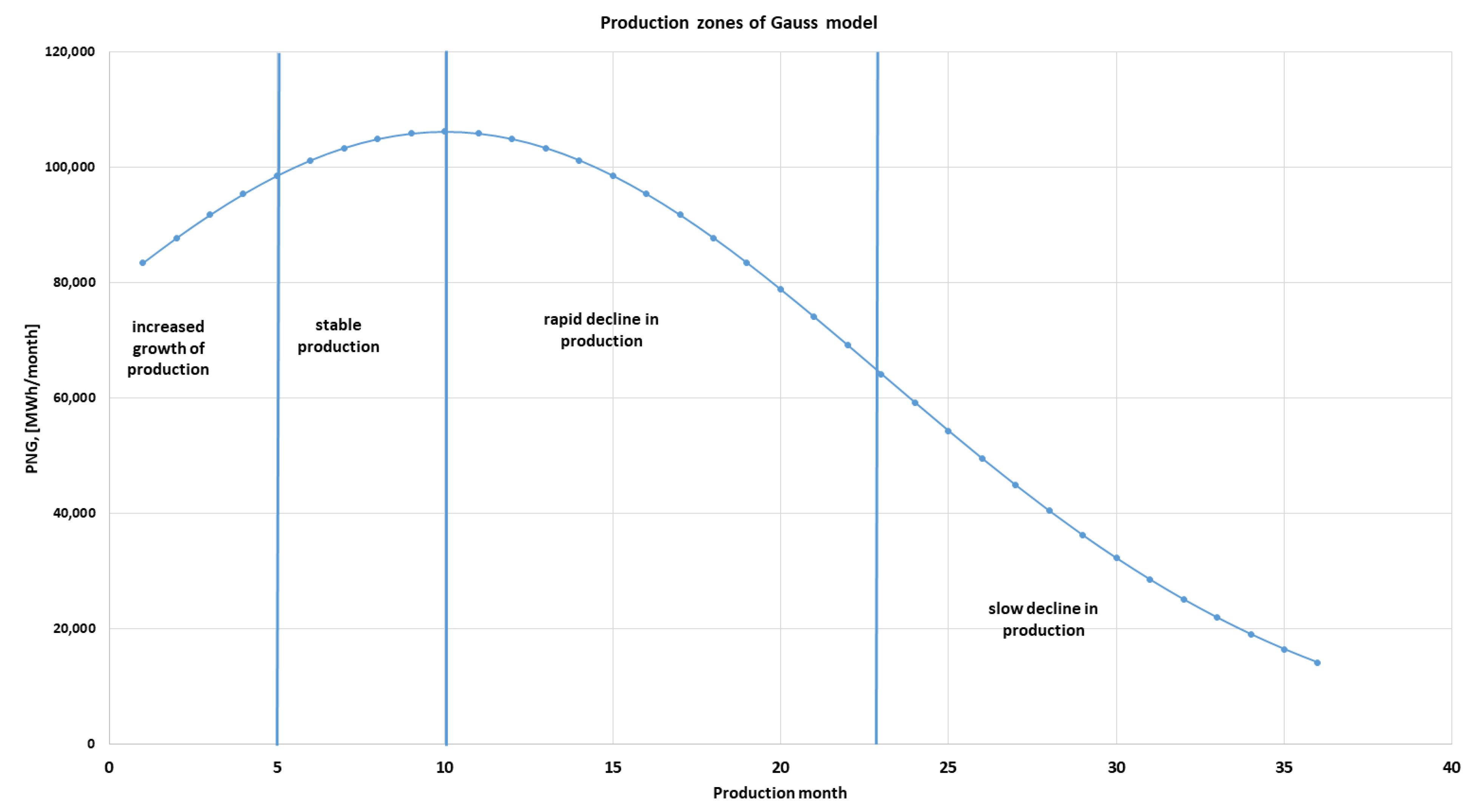
From the Gaussian model [6,37], the following useful elements can be identified in Relation (13); see Table 2. The production phases identified in Figure 9 are the following: increased growth 0–5 months; stable of 5–10 months; rapid decline of 10–23 months; slow decline of 23–36 months.
Table 2.
Gaussian model characteristics.

Figure 9.
Identification of operational areas on the production forecast (PNG, Production of Natural Gas).
The dispersion degree of production calculated with Relation (14) is . For the three situations highlighted above the probabilities of achieving production are
Using the risk matrix, it is possible to identify the area where the future natural gas exploitation will be placed; see Figure 10 [18]. It is noted that the designed well is in level III—a risk zone from the point of view of the possibilities of achieving production in the provided time interval.
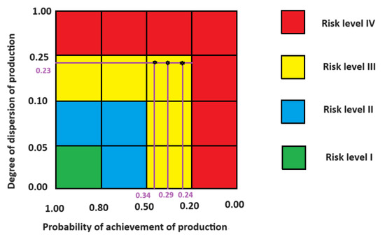
Figure 10.
Risk matrix in the production forecast phase at the gas well.
This model has the advantage of obtaining an associated risk coefficient, but it can also be used to obtain better indications of the relationship between production and the probability of its realization. Relation (13) is considered. In this relationship, the time indicated for each production area is assumed; see Figure 9.
By choosing a moment in time in the fourth phase (slow decrease in production, for example, t = 33 months) we can find out information about the probability of achieving some production in this phase. The values of the variables related to the maximum production, data average, and dispersion are considered variables whose distribution laws are uniform in the following intervals: for the value of the gas volume in the deposit used to establish the maximum production value, this is considered within the limits of [0.95 URR; 1.05 URR], where URR was calculated using Relation (12) for the three values of indicated above; for the mean of the values, the interval is [9.5; 10.5] months; and for the dispersion , the interval is [12.5; 13.5] months. We performed several simulations (1000 values) using the Monte Carlo method to determine the production values.
Sequence 1, used to generate the values for , , and in the Matlab 2022b [37] program, is presented in the Supplementary Materials.
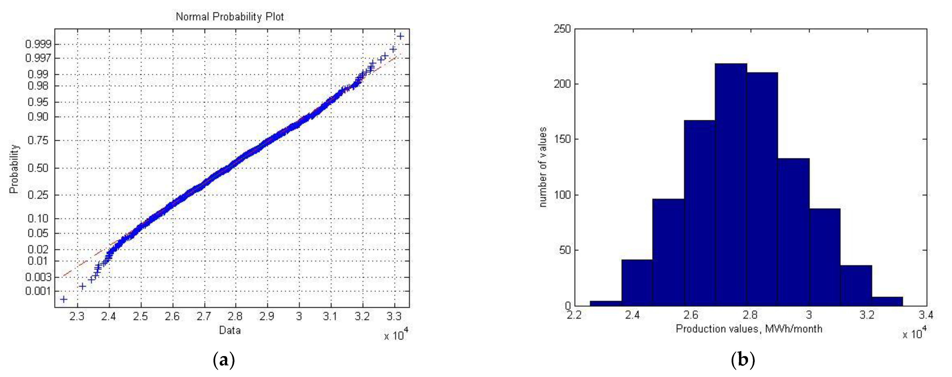
It was verified that the values of obtained with Relation (13) have a normal distribution with the Lillie test and graphical tests (Figure 11) using Matlab sequence 2 from the Supplementary Material [37].

Figure 11.
The graphical tests used to establish the normal distribution for the monthly production value variable Q: (a) normal probability plot; and (b) histogram plot.
For a normal probability plot, if the data points appear along the reference line, the sample data have a normal distribution and aspects checked; see Figure 11a. Histogram representations for gas production values have to be similar to a typical Gauss variation, with aspects checked; see Figure 11b.
We have two possibilities to use the results of a Monte Carlo simulation. First, we compare the production values with a limit value of, for example, 22,000 MWh/month. If the production value is above this level, we record this situation and finally report the number of trials where the production value exceeded this threshold to the total number of trials performed using the Monte Carlo method [19,37]. We roughly find the probability of achieving production above this level by measuring the frequency. Successive trials have some scattering but generally stabilize around a value.
The second possibility that gives us a broader picture of the relationship between production value and its probability is to take the production data obtained by applying the Monte Carlo method and test the distribution law of these data. As can be seen, the ranges in which the variations of the variables on which the model depends are quite narrow, so the production values obtained with Relation (13) are likely to remain around a normal distribution. We checked this aspect with a test, in the present case being the Lillie test (see Supplementary Material [37]), and because the condition of maintaining the null hypothesis was met, we can use the theoretical elements from the normal distribution to establish a link between production and the probability of achievement [16,37]. Graphical tests revealed the same conclusion as in Figure 11. So, we used the second possibility in Figure 12, using Matlab sequence 3.
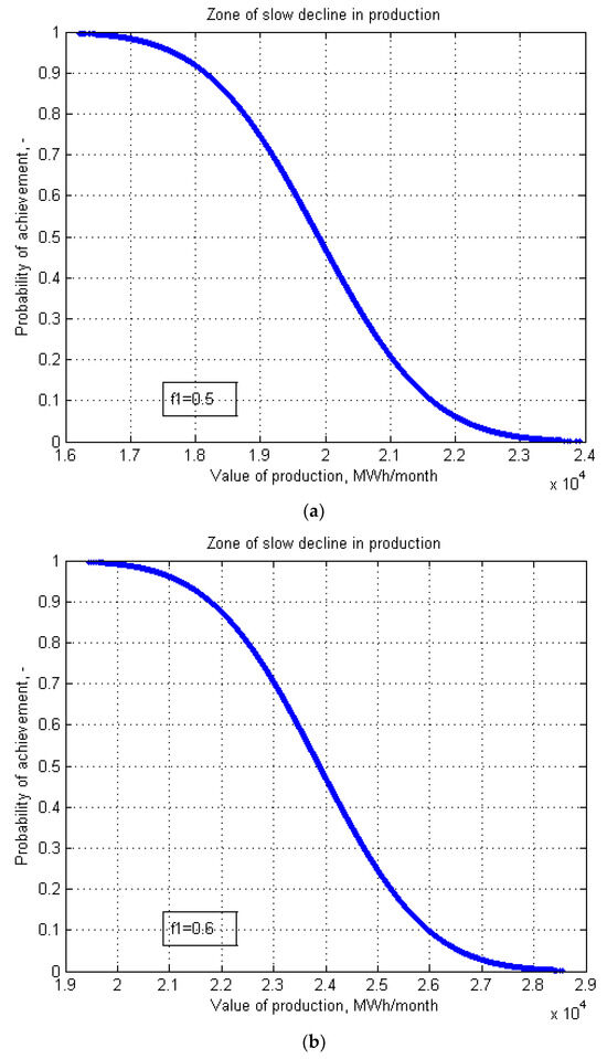

Figure 12.
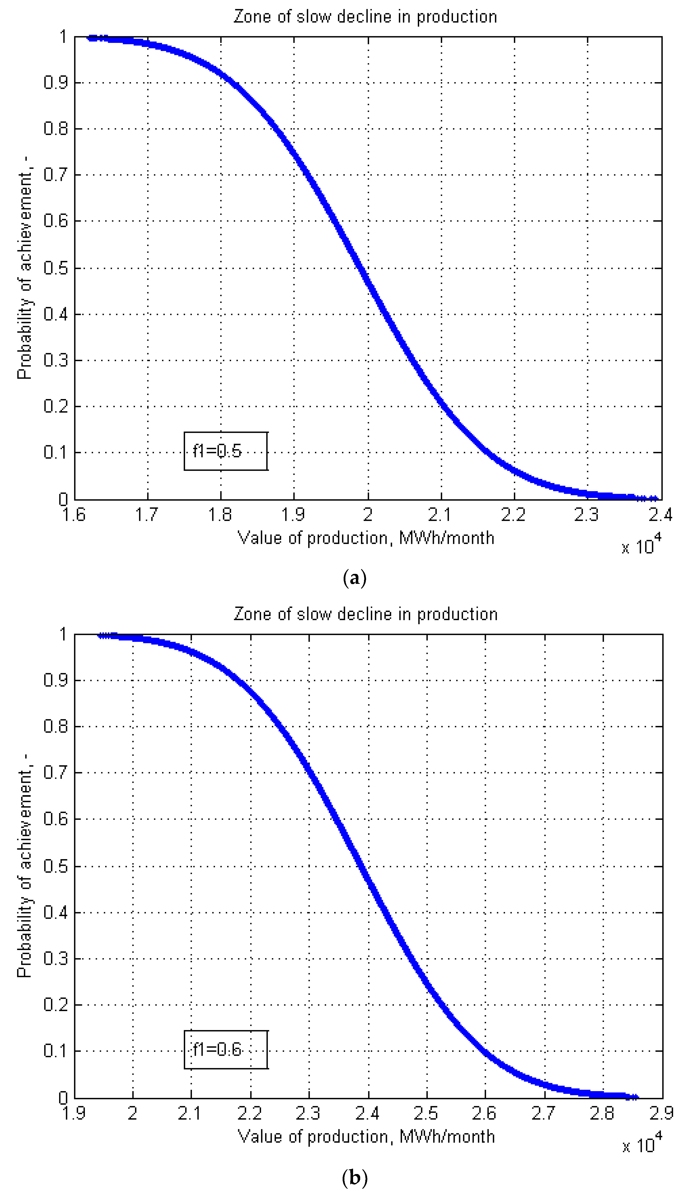
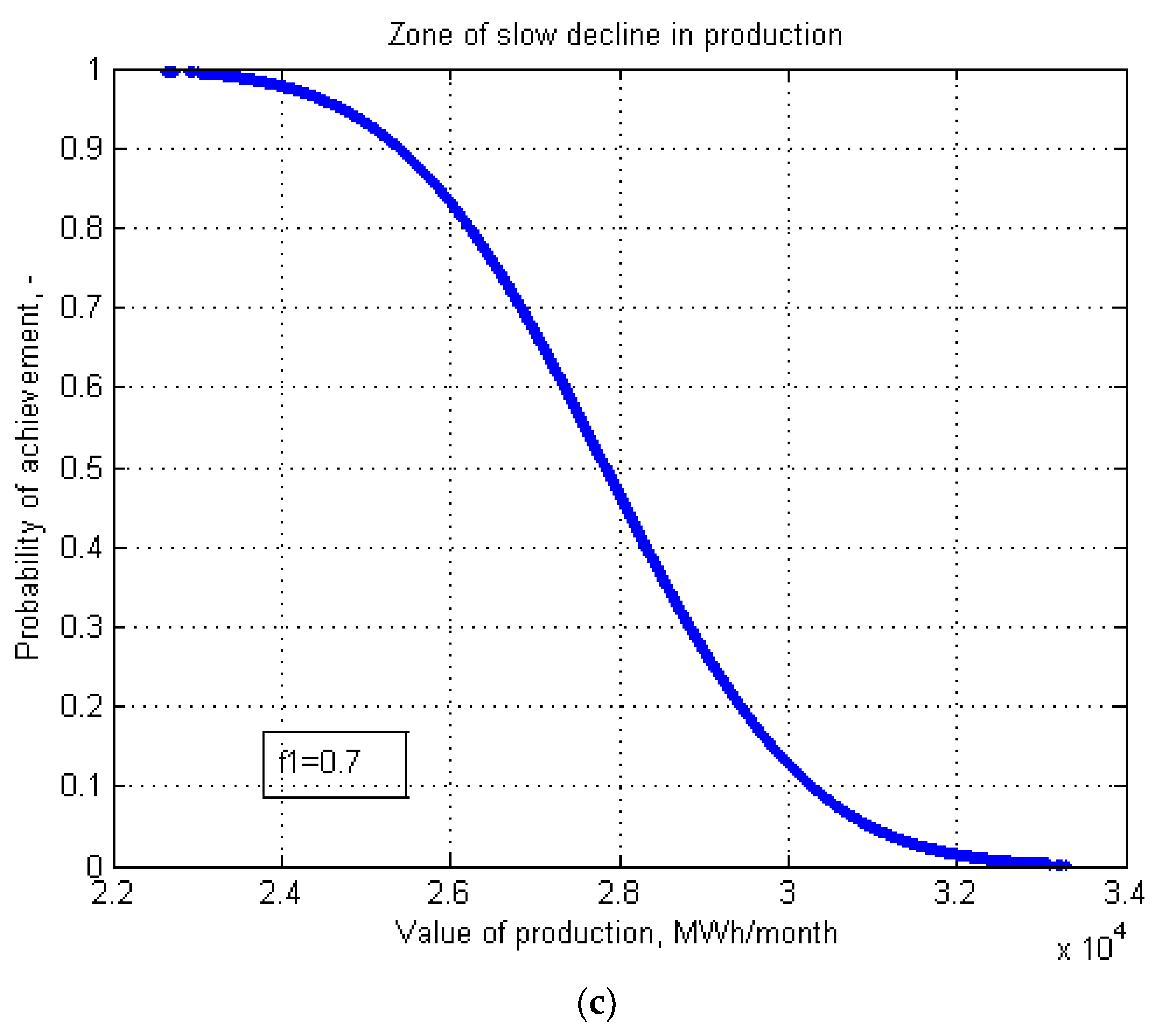
The influence of production on the probability of realization in the phase of slow production decline at a gas well: (a) ; (b) ; and (c) (; ).
For the area of slow production decline, the production achievement probabilities are established according to the production value; see Figure 12 for the following values of the factor: 0.5, 0.6, and 0.7. Assuming that the factor expressing the actual amount of gas in the deposit is half of the amount of gas estimated in the initial investigations, influence of production is shown in the diagram in Figure 12a. Interpreting this diagram, we have a probability of 0.93 of achieving production values greater than 18,000 . In this case, correlating the probability of obtaining a production greater than 18,000 with the production dispersion coefficient of 0.23, we find that we are in the level III risk zone for this operation; see Figure 10. If we want a production of greater than 22,000 in an operation where we have 0.5 ( of the amount of gas predicted in the investigations as the actual volume of gas, a recovery factor of 0.69 , and a technical limitation of 0.72, achieving a production of over 22,000 in the last well exploitation period (in month 33) is very risky, with a probability of 0.05. This means that we do not have enough of a chance to achieve such a production. We are in risk zone level IV.
Figure 12b,c correspond to higher values of proximity between the gas volume determined through investigations and the real gas volume, respectively, 0.6 and 0.7, leading to higher probabilities of achieving productions greater than 22,000 , namely 0.86 and near 1. In these cases, the transition from risk level IV to risk level III is observed in the realization of such production.
This result, based on previous assumptions, tells us more about this exploitation. It can be seen that depending on the production we propose, we have different probabilities of achievement and a certain risk factor.
Similarly, the Hubbert model can be used where we have the following characteristic values: ; ; ; ; and . The symmetric Hubbert model expresses values very close to the Gaussian model. The asymmetric Hubbert model allows production values to approximate the production variation aspect of many gas wells, where the production phase to peak is shorter than the production phase after peak production.
4. Verification of Theoretical Models with Actual Production Data for the X Gas Well
Through Gauss and Hubbert’s theoretical models, well production values were anticipated over a 39-month interval. The risk factor corresponding to this exploitation was also evaluated. That gas well had a continuous exploitation period of 32 months after which production was interrupted for three months. Production was resumed for two months, after which in the following two months, an attempt was made to put the well back into production, but it was abandoned. In conclusion, the production period was 34 months (of 39 months) and is expressed in Table 3. The production values can be compared with the established forecast models and the following conclusions can be drawn from Figure 12. For the use of the two models, the production data provided by the production company are known and shown in Table 3. These data are for the entire duration of the exploitation of the well.
Table 3.
Production data from well X.
The higher calorific value of the gases is 9.9 kWh/Scm.
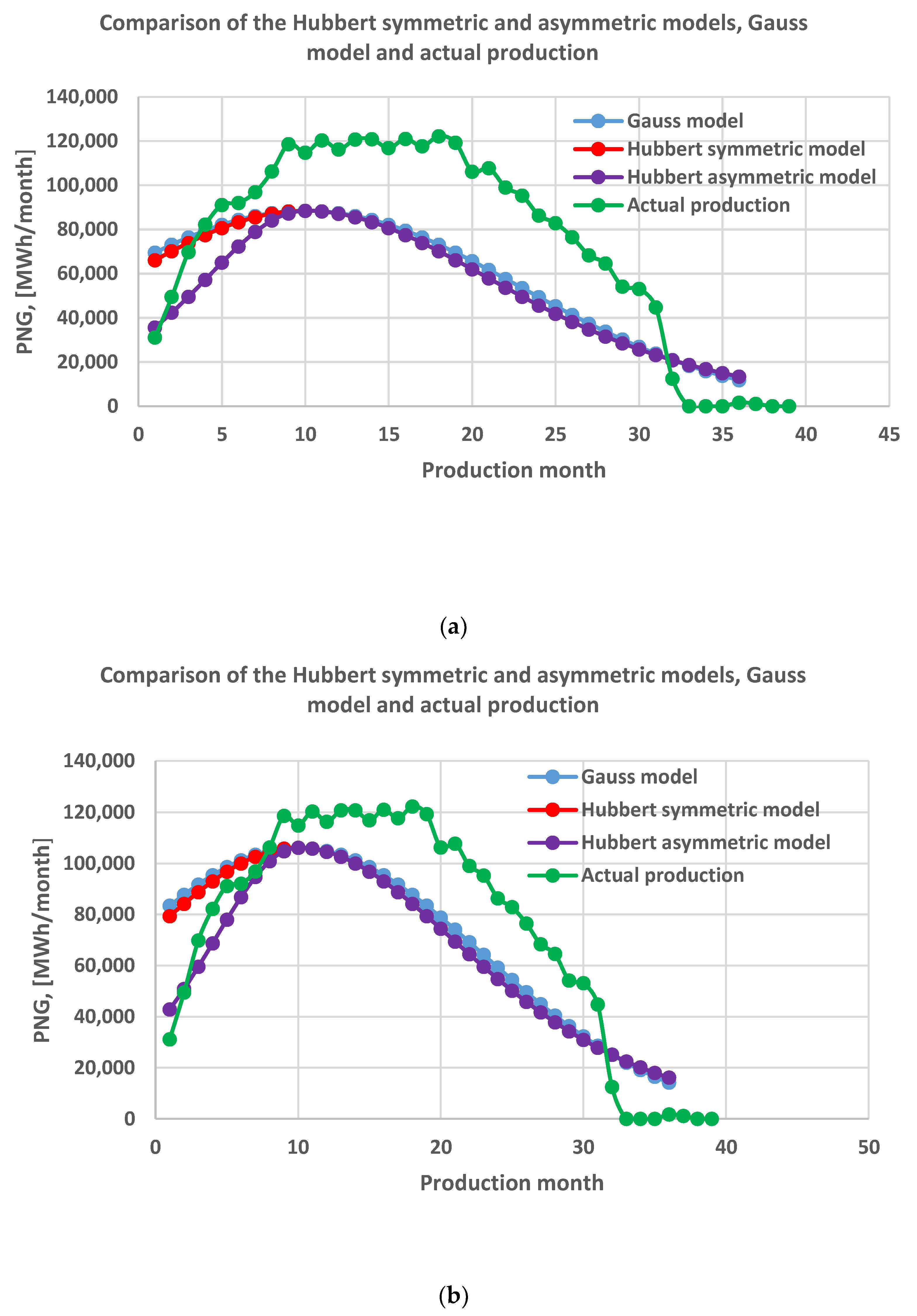
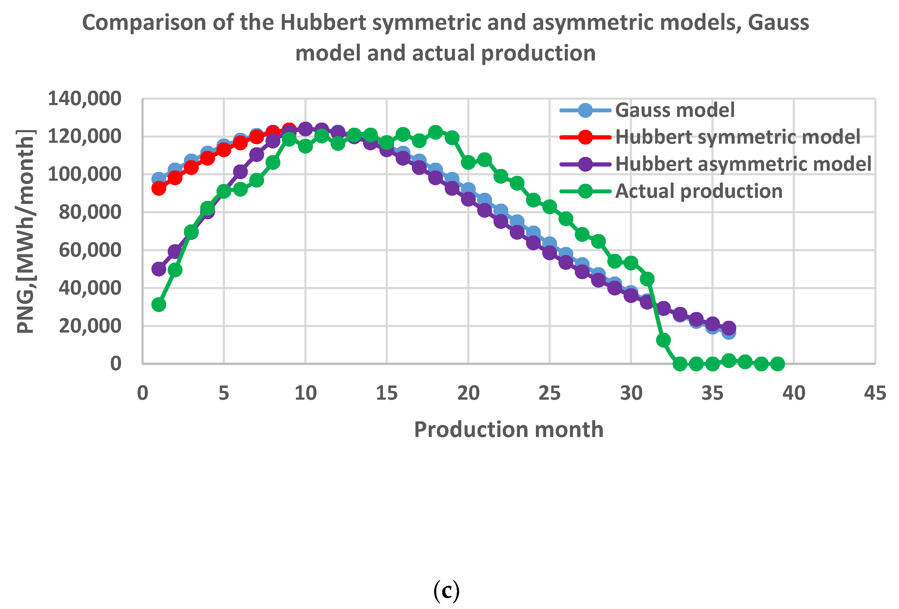
It is observed that the value of the extracted gas volume is within the predicted range of 2.90 × 10⁶ MWh ϵ [2.88 × 10⁶; 4.04 × 10⁶] MWh. Validation of the model with actual production data for this well depends on the factors and From the three situations presented in Figure 13, it can be observed that there is an alignment of the forecast with the production data in the scenario at point c, . A good agreement with the actual values is obtained in the case of Figure 13c on the asymmetric Hubbert model.
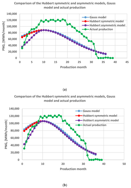

Figure 13.
Comparison between production values and theoretical forecasting models: (a) Gauss model, symmetric/asymmetric Hubbert models, and production values, (b) Gauss model, symmetric/asymmetric Hubbert models, and production values, ; and (c) Gauss model, symmetric/asymmetric Hubbert models, and production values, , (PNG, Production of Natural Gas).
Regarding the difference between the model established using the exponential model (case (b) from Figure 2) for the gas well and the actual production values, it is observed in this case that the difference is very large (2.00 × 10⁶ MWh compared with actual cumulative production 2.90 × 10⁶ MWh), so this production model is inadequate for anticipating the production of gas of this well; see Table 4. The criteria for evaluating forecast models are listed below [37]:
Table 4.
Assessing agreement with forecast models.
- R
- square:
It is recommended that and be as small as possible and that the values of and be close to 1 [37].
5. Conclusions
- Establishing a suitable forecasting model allows the following advantages for a natural gas producer: a. it can predict the cumulative production of a gas well and b. it can appreciate the production values with an accepted risk.These elements ensure the monthly value of the quantities of gas extracted, an essential aspect for the realization of the concluded contracts, and provide in advance the cumulative production that highlights the economic profitability of the project, comparing the costs of making and maintaining the gas well with the revenues.
- The forecasting model used by Romanian companies is almost exclusively the exponential one. It is successfully applied to oil wells. To gas wells, this model has led to numerous failures, which have practically meant missed supply contracts and unprofitable investments.There are three reasons why the traditional pattern of output variations through a continuous decline from a maximum initial value has persisted. The first is related to the difficulty of obtaining information that anticipates production values as well as possible. The second reason is related to the expenses associated with obtaining this information. Thus, we continue to rely on what we already know. Sometimes, the forecasting companies cut their expenses a lot and rely only on the history of the wells in the production area. The third reason is related to the fact that this model has a fairly high frequency of agreement with the results in practice, in particular to oil wells.We note that the exponential model does not give negative results in all situations due to the short period of stable production of (followed by decline in) some gas wells, where this model has been successful.
- The article provides a forecasting alternative for gas wells that leads to better accordance with production value results. The asymmetric Hubbert model offers good possibilities for assessing the behavior of gas wells. This model was adapted according to field observations of gas wells, where the initial production is quite high and rises to the peak level quite quickly. The following changes were introduced: the initial phase of the model was shortened, the slope of the growth period was increased, and the operating interval was shortened.
- The model presented in the article is an attempt to adapt a Hubbert or Gaussian model that is generally applied for long periods and to make these models suitable for a well with a short operating interval. Figure 13 and Table 4 highlighted the results obtained, compared to the actual production of the analyzed gas well.In the exemplified case, the asymmetric Hubert forecast model proved to be the closest to real production conditions from the example presented, it can be seen that there is a good agreement between the forecast model and the real production. The cumulative production values agree quite well with the real production of 2.90 × 10⁶ MWh in the case of Gauss and Hubbert symmetric/asymmetric models 3.04 × 10⁶/2.97 × 106/2.77 × 106 MWh. There is a difference between the cumulative production values of the 2.0e6 MWh exponential model and the actual production values because the exponential model assumes a longer production period (87 months; see Table 1); the exponential model does not agree with the production variation at the exemplified well, according to the comparison indicators in Table 4.
- An interesting attempt to use the Hubbert/Gauss models for gas wells is the work conducted in the Sichuan Basin [18]. The paper presents a way to assess the production and the risk of realizing the forecast at a gas field. Gaussian and symmetric Hubbert models are used. The study period is 60 years: 2010–2070. The model used in this article is adapted to a much shorter production period and with asymmetric behavior.
- There are systems where the characterization is based on little data. The gray systems theory is a useful tool for solving uncertain problems with limited data. The new GMTGP (Gray Model Tight Gas Production) model presented in [16] solves the problem of reasonably predicting tight gas production in China. However, it may not be suitable for predicting other unconventional gas production. So, we must adapt the models to the situations in the field. The selection of gray models must be based on the data characteristics of the modeling system; otherwise, it is difficult to achieve satisfactory model accuracy. Specifically, this model GMTGP makes a prediction for the years 2018–2020 based on tight gas production data throughout China between 2009 and 2017. The present article uses a similar approach based on field situations as in Figure 8: fit classical models based on sparse information. The article succeeds in pointing to a better model for the cases it deals with.
- The use of artificial neural network, ANN, models is based on training datasets to determine the network followed by solving test cases [17]. The method of neural networks is also a way to approach forecasting. The method is based on varied data specific to an area, which in many situations makes it difficult to determine what constitutes an impediment. The team carrying out this work proposes a continuation of the study in this direction.
- It is also intended to change the opinion of gas producers on their exclusive use of the exponential model. This may lead to large errors in the gas production forecasting.
Supplementary Materials
The following supporting information can be downloaded at https://www.mdpi.com/article/10.3390/pr12051009/s1.
Author Contributions
Conceptualization, A.P.P., I.P., I.G.S. and C.N.E.; methodology, A.P.P., I.P., I.G.S. and C.N.E.; software, I.P. and C.N.E.; validation, A.P.P., I.P., I.G.S., C.N.E., D.B.S. and I.V.G.; formal analysis, A.P.P., I.P., I.G.S. and C.N.E.; investigation, I.P., I.G.S., C.N.E., D.B.S. and I.V.G.; resources, A.P.P., I.P., I.G.S., C.N.E., D.B.S. and I.V.G.; data curation, I.P., I.G.S. and I.V.G.; writing—original draft preparation, A.P.P., I.P., I.G.S. and C.N.E.; writing—review and editing, C.N.E., D.B.S. and I.V.G.; visualization, A.P.P., I.P., I.G.S., C.N.E., D.B.S. and I.V.G.; supervision, A.P.P. and I.P.; project administration, A.P.P.; funding acquisition, A.P.P. All authors have read and agreed to the published version of the manuscript.
Funding
This research was funded by the Petroleum-Gas University of Ploiesti for the Study of the possibilities of increasing the storage/extraction capacity of natural gas in an underground storage, no. 11065/08.06.2023.
Data Availability Statement
Other data are not available due to the confidentiality clause in the contracts with the natural gas producers who supported this work.
Conflicts of Interest
The authors declare no conflicts of interest.
Abbreviation
Nomenclature
| is the cumulative natural gas production, ; | |
| mean squared error, ; | |
| maximum monthly production of natural gas, ; | |
| initial value of the average gas flow that can be obtained daily, ; | |
| is the average daily gas flow production in the month , ; | |
| is the average monthly gas flow production in the month , ; | |
| root mean squared error, ; | |
| is the sum of the squares of the differences between the values of the variable and the values on the regression curve, ; | |
| is the sum of the squares of the differences between the values of the variable and their mean value, ; | |
| is the value of the ultimate recoverable resource from the gas deposit, ; | |
| the slope corresponding to periods of increased or decreased production, at Hubbert model ; | |
| decline factor at exponential model, ; | |
| hyperbolic cosine, ; | |
| is the number of coefficients used to determine the approximation curve of the model values; | |
| is the number of production months; | |
| production month, month; | |
| means the time at which the production peak is reached, ; | |
| is the standard deviation for the Gauss model, ; | |
| is the average value of production time for the Gauss model, . |
References
- Resnikoff, M. Radon in Natural Gas from Marcellus Shale. Ethics Biol. Eng. Med. 2011, 2, 317–331. [Google Scholar] [CrossRef]
- Wang, C.; Liu, Y.; Yu, C.; Zheng, Y.; Wang, G. Dynamic risk analysis of offshore natural gas hydrates depressurization production test based on fuzzy CREAM and DBN-GO combined method. J. Nat. Gas Sci. Eng. 2021, 91, 103961. [Google Scholar] [CrossRef]
- Cavallo, A.J. Predicting the Peak in World Oil Production. Nat. Resour. Res. 2002, 11, 187–195. [Google Scholar] [CrossRef]
- Li, N.; Wang, J.; Wu, L.; Bentley, Y. Predicting monthly natural gas production in China using a novel grey seasonal model with particle swarm optimization. Energy 2021, 215, 119118. [Google Scholar] [CrossRef]
- Qiao, W.; Liu, W.; Liu, E. A combination model based on wavelet transform for predicting the difference between monthly natural gas production and consumption of U.S. Energy 2021, 235, 121216. [Google Scholar] [CrossRef]
- Wang, X.; Lei, Y.; Ge, J.; Wu, S. Production forecast of China׳s rare earths based on the Generalized Weng model and policy recommendations. Resour. Policy 2015, 43, 11–18. [Google Scholar] [CrossRef]
- Maggio, G.; Cacciola, G. A variant of the Hubbert curve for world oil production forecasts. Energy Policy 2009, 37, 4761–4770. [Google Scholar] [CrossRef]
- Gallagher, B. Peak oil analyzed with a logistic function and idealized Hubbert curve. Energy Policy 2011, 39, 790–802. [Google Scholar] [CrossRef]
- Nogueira Hallack, L.; Salem Szklo, A.; Olímpio Pereira Júnior, A.; Schmidt, J. Curve-fitting variants to model Brazil’s crude oil offshore post-salt production. J. Pet. Sci. Eng. 2017, 159, 230–243. [Google Scholar] [CrossRef]
- Kosova, R.; Xhafaj, E.; Qendraj, D.H.; Prifti, I. Forecasting Fossil Fuel Production Through Curve-Fitting Models: An Evaluation of the Hubbert Model. Math. Model. Eng. Probl. 2023, 10, 1149–1156. [Google Scholar] [CrossRef]
- Setiawan; Dahlan, R.; Zulkarnain, I.; Prayoga, A.; Budiawan, Y. Asymmetric Hubbert Curve in Indonesia Oil Production. In Ametis Institute 2017, Working Paper Series No. 61.; SSRN: Rochester, NY, USA; Available online: https://ssrn.com/abstract=3010091 (accessed on 12 May 2024).
- Hubbert, M.K. Energy Resources; The National Academies Press: Washington, DC, USA, 1962; p. 153. [Google Scholar]
- Tilton, J.E. The Hubbert peak model and assessing the threat of mineral depletion. Resour. Conserv. Recycl. 2018, 139, 280–286. [Google Scholar] [CrossRef]
- Zhang, P.; Zhang, Y.; Zhang, W.; Tian, S. Numerical simulation of gas production from natural gas hydrate deposits with multi-branch wells: Influence of reservoir properties. Energy 2022, 238, 121738. [Google Scholar] [CrossRef]
- Wang, J.; Liu, J.; Li, Z.; Li, H.; Zhang, J.; Li, W.; Zhang, Y.; Ping, Y.; Yang, H.; Wang, P. Synchronous injection-production energy replenishment for a horizontal well in an ultra-low permeability sandstone reservoir: A case study of Changqing oilfield in Ordos Basin, NW China. Pet. Explor. Dev. 2020, 47, 827–835. [Google Scholar] [CrossRef]
- Zeng, B.; Ma, X.; Zhou, M. A new-structure grey Verhulst model for China’s tight gas production forecasting. Appl. Soft Comput. 2020, 96, 106600. [Google Scholar] [CrossRef]
- Bataee, M.; Irawan, S.; Kamyab, M. Artificial Neural Network Model for Prediction of Drilling Rate of Penetration and Optimization of Parameters. J. Jpn. Pet. Inst. 2014, 57, 65–70. [Google Scholar] [CrossRef]
- Yu, G.; Chen, Y.; Li, H.; Liu, L.; Wang, C.; Chen, Y.; Zhang, D. Studies on natural gas production prediction and risk quantification of Sinian gas reservoir in Sichuan Basin. J. Pet. Explor. Prod. Technol. 2021, 12, 1109–1120. [Google Scholar] [CrossRef]
- Dheskali, E.; Koutinas, A.A.; Kookos, I.K. Risk assessment modeling of bio-based chemicals economics based on Monte-Carlo simulations. Chem. Eng. Res. Des. 2020, 163, 273–280. [Google Scholar] [CrossRef]
- Mehana, M.; Callard, J.; Kang, Q.; Viswanathan, H. Monte Carlo simulation and production analysis for ultimate recovery estimation of shale wells. J. Nat. Gas Sci. Eng. 2020, 83, 103584. [Google Scholar] [CrossRef]
- Wang, N.; Zhao, Q.; Guo, W.; Zang, H.; Liu, D. Application of the Monte Carlo Simulation in evaluating unconventional gas well economy. In Proceedings of the 2016 5th International Conference on Sustainable Energy and Environment Engineering (ICSEEE 2016), Zhuhai, China, 12–13 November 2016; pp. 978–981. [Google Scholar]
- Davis, J.C.; Harbaugh, J.W. Statistical evaluation of oil and gas prospects in the outer continental shelf of the U.S. Gulf Coast. J. Int. Assoc. Math. Geol. 1983, 15, 217. [Google Scholar] [CrossRef]
- Jia, A. Progress and prospects of natural gas development technologies in China. Nat. Gas Ind. B 2018, 5, 547–557. [Google Scholar] [CrossRef]
- Yadua, A.U.; Lawal, K.A.; Okoh, O.M.; Ovuru, M.I.; Eyitayo, S.I.; Matemilola, S.; Obi, C.C. Stability and stable production limit of an oil production well. J. Pet. Explor. Prod. Technol. 2020, 10, 3673–3687. [Google Scholar] [CrossRef]
- Klemetsdal, Ø.S.; Rasmussen, A.F.; Møyner, O.; Lie, K.-A. Efficient reordered nonlinear Gauss–Seidel solvers with higher order for black-oil models. Comput. Geosci. 2019, 24, 593–607. [Google Scholar] [CrossRef]
- Cao, H.; Mohareb, M.; Nistor, I. Partitioned water hammer modeling using the block Gauss–Seidel algorithm. J. Fluids Struct. 2021, 103, 103260. [Google Scholar] [CrossRef]
- Boumi Mfoubat, H.R.N.; Zaky, E.I. Optimization of waterflooding performance by using finite volume-based flow diagnostics simulation. J. Pet. Explor. Prod. Technol. 2019, 10, 943–957. [Google Scholar] [CrossRef]
- Li, H.; Yu, G.; Fang, Y.; Chen, Y.; Wang, C.; Zhang, D. Studies on natural gas reserves multi-cycle growth law in Sichuan Basin based on multi-peak identification and peak parameter prediction. J. Pet. Explor. Prod. Technol. 2021, 11, 3239–3253. [Google Scholar] [CrossRef]
- Jones, T.H.; Willms, N.B.; Ingram, P. A critique of Hubbert’s model for peak oil. Facets 2018, 3, 260–274. [Google Scholar] [CrossRef]
- Helias, A.; Heijungs, R. Resource depletion potentials from bottom-up models: Population dynamics and the Hubbert peak theory. Sci. Total Environ. 2019, 650, 1303–1308. [Google Scholar] [CrossRef] [PubMed]
- Ebrahimi, M.; Cheshme Ghasabani, N. Forecasting OPEC crude oil production using a variant Multicyclic Hubbert Model. J. Pet. Sci. Eng. 2015, 133, 818–823. [Google Scholar] [CrossRef]
- Peng, W.; Guo, F.; Hu, G.; Lyu, Y.; Gong, D.; Liu, J.; Feng, Z.; Guo, J.; Guo, Y.; Han, W. Geochemistry and accumulation process of natural gas in the Shenmu Gas Field, Ordos Basin, central China. J. Pet. Sci. Eng. 2019, 180, 1022–1033. [Google Scholar] [CrossRef]
- Liu, H.; Tang, Y.; Chen, K.; Tang, W. Erratum to: The tectonic uplift since the Late Cretaceous and its impact on the preservation of hydrocarbon in southeastern Sichuan Basin, China. J. Pet. Explor. Prod. Technol. 2017, 7, 463. [Google Scholar] [CrossRef]
- Yang, Y.; Yang, Y.; Wen, L.; Zhang, X.; Chen, C.; Chen, K.; Zhang, Y.; Di, G.; Wang, H.; Xie, C. New progress and prospect of Middle Permian natural gas exploration in the Sichuan Basin. Nat. Gas Ind. B 2021, 8, 35–47. [Google Scholar] [CrossRef]
- Zhi, D.; Song, Y.; Zheng, M.; Qin, Z.; Gong, D. Genetic types, origins, and accumulation process of natural gas from the southwestern Junggar Basin: New implications for natural gas exploration potential. Mar. Pet. Geol. 2021, 123, 104727. [Google Scholar] [CrossRef]
- Sun, Y.-L.; Rahmani, A.; Saeed, T.; Zarringhalam, M.; Ibrahim, M.; Toghraie, D. Simulation of deformation and decomposition of droplets exposed to electro-hydrodynamic flow in a porous media by lattice Boltzmann method. Alex. Eng. J. 2022, 61, 631–646. [Google Scholar] [CrossRef]
- The MathWorks, I. MATLAB. Available online: https://www.mathworks.com (accessed on 3 January 2024).


Disclaimer/Publisher’s Note: The statements, opinions and data contained in all publications are solely those of the individual author(s) and contributor(s) and not of MDPI and/or the editor(s). MDPI and/or the editor(s) disclaim responsibility for any injury to people or property resulting from any ideas, methods, instructions or products referred to in the content. |
© 2024 by the authors. Licensee MDPI, Basel, Switzerland. This article is an open access article distributed under the terms and conditions of the Creative Commons Attribution (CC BY) license (https://creativecommons.org/licenses/by/4.0/).