Abstract
To address the significant challenges in determining the single-well production of tight gas and shale gas after hydraulic fracturing, artificial intelligence (AI) methods were implemented. Machine learning (ML) algorithms such as random forest (RF), extremely randomized trees (ET), lightweight gradient boosting machines (LightGBM), gradient boosting regression (GBR), and linear regression (LR) were utilized in conjunction with reservoir geology, engineering parameters, and production data to develop several foundational models for forecasting the production of unconventional gas wells. The accuracy of these models was evaluated. Based on this, improvements in the models’ predictive accuracy and generalizability were achieved through the ensemble of machine learning models. Furthermore, this paper selected two representative tight and shale gas reservoirs to demonstrate the application of the ensemble model for well production forecasting, and a comparative analysis with actual production data was conducted. For tight gas reservoir A, the blending model achieved an MAE of 0.8419 and an MSE of 1.0930, with an R2 score of 0.8812. For shale gas reservoir B, the blending model achieved an MAE of 1.4841 and an MSE of 3.1629, with an R2 score of 0.9524. The results of the case studies indicate that the ensemble model approach employed in this study has a higher predictive accuracy and reliability than a single machine learning algorithm, and is capable of handling high-dimensional, large-scale, and imbalanced data, offering scientific validation and technical support for the assessment of the well productivity in tight and shale gas wells.
1. Introduction
Currently, tight gas and shale gas reservoirs are increasingly recognized as significant contributors to the overall energy resources, complementing the traditional oil reservoirs. However, unconventional gas reservoirs such as tight gas and shale gas generally have characteristics such as low porosity, ultra-low permeability, and strong heterogeneity. They do not have natural productivity, and it is almost impossible to obtain an industrial gas flow without using fracturing measures. Moreover, the fracture pattern formed by multi-stage fracturing or volume fracturing is very complex, and the flow characteristics are not clear, which increases the difficulty of predicting single-well production [1,2,3,4,5,6,7,8,9,10].
In recent years, scholars from both China and other major gas-producing regions, including North America, have conducted extensive research on the prediction of production rates in tight gas and shale gas wells, using methods such as empirical formulas, analytical models, and numerical simulations [11,12,13,14,15,16]. Empirical formulas and analytical models are mainly based on theoretical models, which make it difficult to fully consider the complex flow characteristics of unconventional gas reservoirs. Furthermore, different models have different applicable conditions, resulting in significant deviations in the prediction results. Numerical models usually simplify the actual reservoir characteristics, making it challenging to accurately characterize the complex reservoir structure and dynamic fracture networks, leading to significant uncertainties in the prediction results. Therefore, it is necessary to explore integrated learning models for predicting the single-well production in unconventional gas reservoirs.
Machine learning is a branch of artificial intelligence that enables computers to learn patterns and models from data without the need for explicit programming. The fundamental principle of machine learning is the use of mathematical and statistical methods to construct mathematical models. These models are adjusted through optimization algorithms to best fit the data and generalize to new data. Common machine learning algorithms include multiple linear regression, decision trees, random forests, support vector machines, neural networks, and so on. Machine learning can delve into data to discover the underlying patterns and handle complex nonlinear relationships, and is characterized by high computational accuracy and the ease of application. It is also applicable in the field of oil and gas development.
Recently, scholars have conducted a series of studies using machine learning methods for single-well production prediction in unconventional gas reservoirs. In 2015, Ma established a sample set of influencing factors on production capacity [17]. They used BP neural network and support vector machine methods to predict the production rate of tight gas wells. The relative error of the support vector machine method ranged from 7.06% to 19.59%, while the relative error of the BP neural network ranged from 8.49% to 37.79%. In 2016, Tian et al., based on an improved BP neural network, established a shale gas production prediction model with production time, cumulative gas production, and reservoir pressure as the input layer, and gas production as the output layer [18]. The relative error prediction was 8.2%. In 2017, Zhu et al. used an adaptive threshold denoising algorithm to remove noise and then applied the BP neural network to nonlinearly fit the reservoir transformation data, thereby obtaining a production prediction model for shale gas wells [19]. Compared to the traditional BP neural network, this model showed improvements in accuracy and stability. In 2019, Lu used reservoir thickness, porosity, permeability, saturation, tubing pressure, water–gas ratio, and other constraints. They established production prediction models using recurrent neural networks and long short-term memory neural networks [20]. The average relative error of the prediction results was less than 10%. Ma et al. proposed a machine learning-based method for the uncertain prediction of shale gas production capacity using a combination of maximum information coefficient correlation analysis, a hybrid support vector machine technique, and Markov chain Monte Carlo simulation [21]. An analysis of 24 shale gas well examples showed an accuracy rate of 70.8% using this method. Fan et al. used the gray correlation method to determine the main controlling factors and weights of shale gas wells [22]. They then used a BP neural network method optimized by genetic algorithms and combined it with data mining techniques to fully utilize the geological and engineering parameters. They established a shale gas rate prediction model for horizontal wells with volume fracturing, with an average prediction error of 8.76%. In 2020, Li et al. used a NARX neural network based on a time series to establish a production rate prediction model between oil pressure and production, with a prediction accuracy of up to 90% in one year of production time [23]. Chen et al. used a genetic algorithm to optimize the weight and threshold of the BP neural network and established a gas rate prediction model for shale gas horizontal wells with volume fracturing [24]. Zhao et al. used horizontal gas wells as training samples and constructed a production prediction model for horizontal wells using the BP neural network and a support vector machine [25]. The research results showed that the support vector machine had a higher prediction accuracy than the BP neural network, with a prediction accuracy of 90% for the absolute open flow rate. Yan et al., based on actual data from the Fuling shale gas wells, established a shale gas production prediction model using deep neural networks, support vector machines, and extreme gradient boosting methods, and analyzed the advantages, disadvantages, and importance of various models [26]. He et al. considered the geological factors and engineering factors comprehensively based on machine learning methods [27]. They applied the random forest method to predict the shale gas well production rate, achieving an accuracy of over 90% in the prediction results. Currently, previous studies mainly rely on a single machine learning model to predict the single-well production rate in unconventional gas reservoirs, which has certain feasibility but further improvement is needed in terms of the accuracy and stability of production prediction.
Ensemble learning is a machine learning method that leverages the strengths of multiple different learners and combines their outputs through certain strategies to achieve better results than by individual learners. The advantages of ensemble learning include reducing the risk of overfitting, improving the generalization ability, and handling high-dimensional, large-scale, and imbalanced data [28]. In this study, for the challenging task of determining the single-well production rate in tight gas and shale gas, machine learning algorithms such as random forest (RF), extremely randomized trees (ET), LightGBM (light gradient boosting machine), gradient boosting regression (GBR), and linear regression (LR) were used. We selected these algorithms due to their proven effectiveness in handling high-dimensional data and capturing the complex non-linear relationships inherent in reservoir and production data. These models are particularly adept at dealing with the imbalanced and noisy nature of the datasets typically encountered in gas production prediction tasks [29,30,31,32]. By integrating geological, reservoir, engineering parameters, and production data, several basic models for predicting the production in unconventional gas single wells was established, and the accuracy of each model was validated. Based on the predictions of multiple basic models, ensemble machine learning was employed to further improve the accuracy and generalization ability of the prediction model. This method can effectively utilize existing data resources to enhance the understanding and evaluation of tight gas reservoirs, providing a scientific basis for optimizing the development plans and improving the production efficiency.
2. Process for Predicting the Gas Rate in Unconventional Gas Reservoirs
Predicting the gas production rates in unconventional gas reservoirs involves understanding the fundamental principles of reservoir engineering and fluid dynamics. Unconventional reservoirs, such as shale gas and tight gas, have unique characteristics that influence the gas flow and production rates. Machine learning models enhance the traditional prediction methods by leveraging large datasets and identifying complex patterns that may not be apparent through conventional techniques. By incorporating features such as: (1) reservoir properties: porosity, permeability, and saturation; (2) operational parameters: pressure, temperature, and number of fracturing stages; (3) historical production data: past production rates and decline trends.
Machine learning models can provide more accurate and robust predictions. In this study, we employed models such as random forest (RF), extremely randomized trees (ET), light gradient boosting machine (LightGBM), gradient boosting regression (GBR), and linear regression (LR). These models were chosen for their ability to handle non-linearity, the interactions among variables, and high-dimensional data. By integrating these theoretical principles with advanced machine learning techniques, our approach aims to deliver precise gas production forecasts, which are crucial for optimizing field development and management strategies.
The main steps for predicting single-well production in unconventional gas reservoirs based on artificial intelligence analysis are as follows:
- (1)
- Data collection and cleaning. Gather relevant data on the geology, reservoirs, and engineering, perform quality checks on the data, handle abnormal values and missing values, and normalize or standardize the data.
- (2)
- Feature engineering and dimensionality reduction. Based on the characteristics of the dataset, select appropriate methods to extract the features specific to tight gas and shale gas rates, transforming high-dimensional raw data into low-dimensional feature vectors to reduce the redundant information and noise interference.
- (3)
- Model construction and training. Choose multiple machine learning models according to the prediction objectives and problem types, utilize the historical data of known production as the training set, optimize and fit the model parameters, and evaluate the generalization ability of the models using metrics such as Mean Absolute Error (MAE) and Mean Squared Error (MSE).
- (4)
- Production rate prediction and result analysis. Utilize the trained model to predict the production rate of the testing set and compare it with the actually observed values. Adjust or improve the above models based on the accuracy and stability of the prediction results.
- (5)
- Ensemble of machine learning models. To further enhance the accuracy of the production rate predictions, ensemble learning can be used to integrate the prediction results of multiple base models, improving the generalization ability and accuracy of the machine learning models.
3. Production Rate Prediction in Tight Gas Field A
3.1. Overview
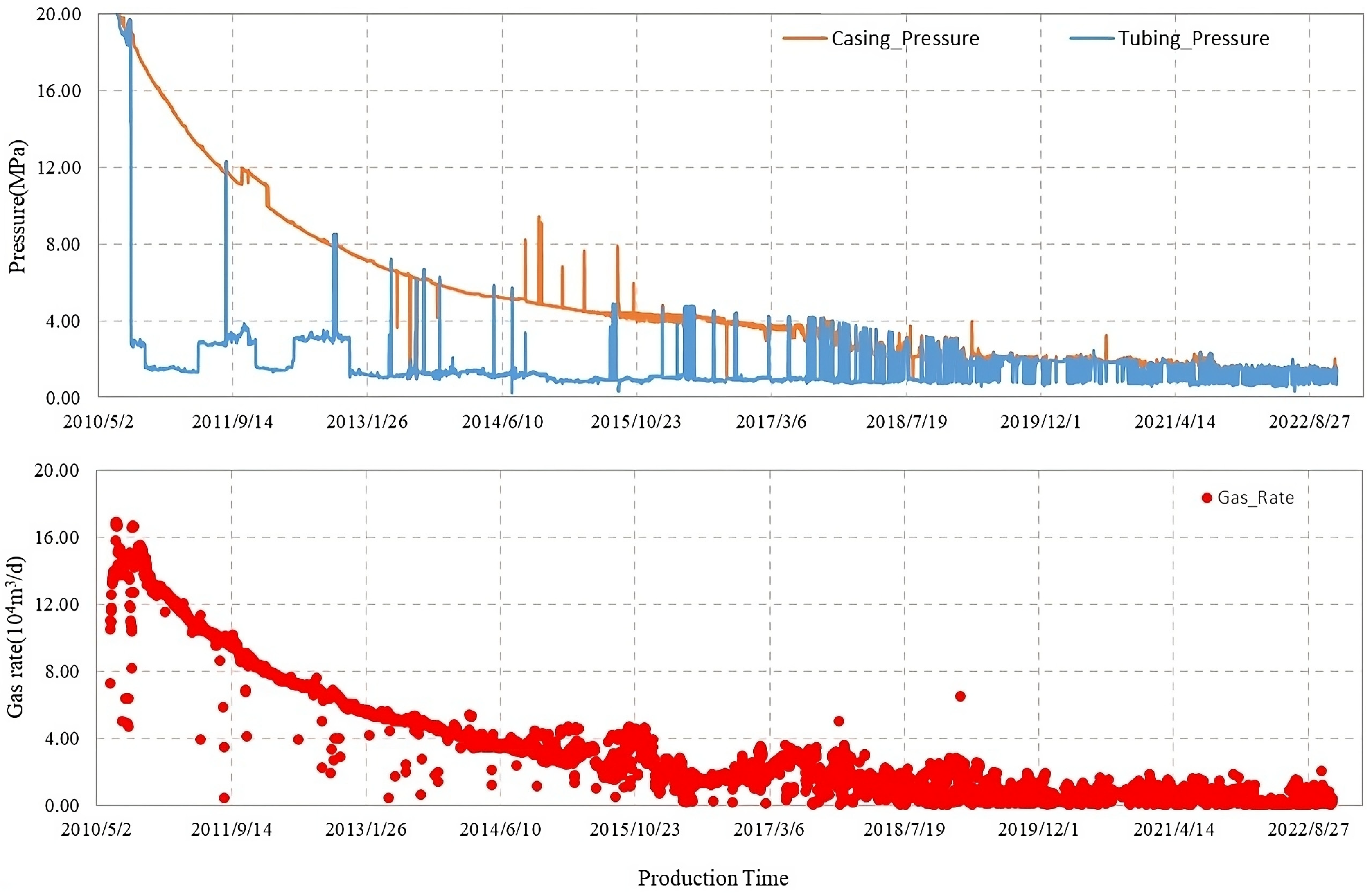
Gas Field A had a depth of 10,499–11,483 ft and an average effective thickness of 31 ft in the gas reservoir. The porosity ranged from 5.0% to 10.0%, and the average permeability was 0.82 mD. The pressure coefficient ranged from 0.87 to 0.94, and the temperature of the gas reservoir was between 100 and 110 °C. Starting from 2010, the field has been developed through the implementation of horizontal well development using a 3937 × 1969 ft irregular rhombus-shaped well pattern. Fracturing treatments are mainly conducted using open-hole packers for zonal isolation and supplemented with multiple fractures or volume fracturing within each section. The total injecting fluid volume per well ranged from 29.1 to 256.6 mcf, with an average of 120.8 mcf. The total sand volume per well ranged from 3.0 to 28.0 mcf, with an average of 13.7 mcf. The initial production rates of over 200 wells in the study area ranged from 0.8 to 7.4 mmcf/d. Figure 1 shows the typical production curve of a single well in Gas Field A.
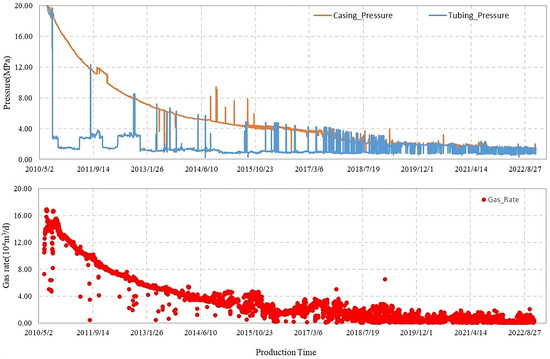
Figure 1.
Typical production curve of deviated wells in Gas Field A.
3.2. Data Processing and Preparation
Data processing and preparation are complex and meticulous processes that require the selection of appropriate tools and techniques based on different data types and scenarios to achieve the optimal results. In the feature selection process, we incorporated both analytical insights and significant physical parameters critical to gas production, such as reservoir, geological parameters, and operational parameters. This holistic approach ensures that our model captures essential factors influencing the production rates, thereby enhancing the model’s predictive accuracy and validity.
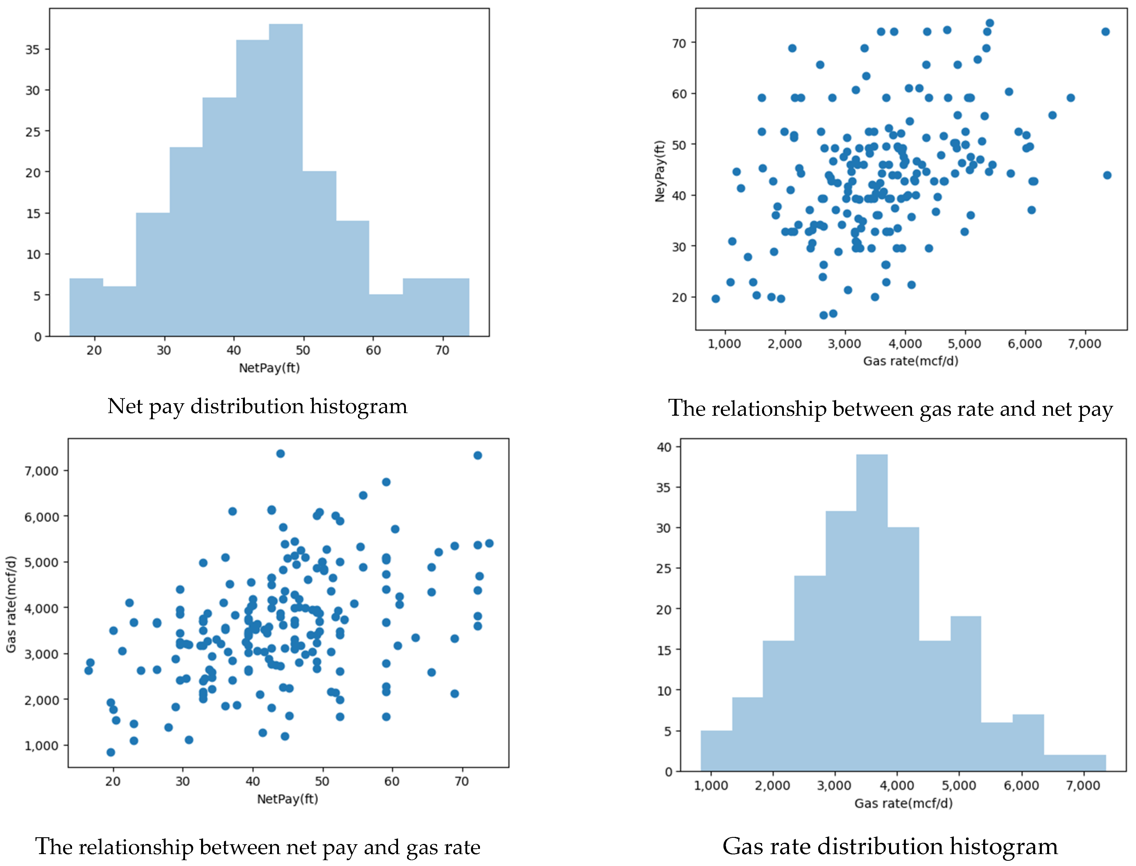
Geological reservoir parameters, engineering parameters, and production data were collected from over 200 wells in Gas Field A, resulting in the acquisition of the raw dataset. Some of the raw data (3.6%) were missing and were filled in using the interpolation method, while abnormal values were treated accordingly. The dataset consisted of 21 data features, and using all features for training in the model would significantly increase its complexity and computational time. This study utilized pairwise relationship graphs to visualize the relationships between two variables, assessing both the single-well production rate and the 21 features, as well as evaluating whether there were significant correlations among the 21 feature parameters. Figure 2 analyzes the pairwise relationship graph between the gas production rate and effective thickness.
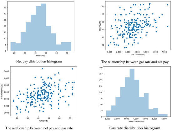
Figure 2.
Pair plot between gas rate and effective thickness in tight gas reservoirs.
After the analysis, the factors with a poor correlation to the production rate were removed to ensure both a sufficient data volume and improved computational efficiency. The processed dataset included 13 factors that are significantly related to the production rate, including the reservoir type, effective thickness, porosity, average gas saturation, length of the horizontal section, length of the fractured section, total fluid volume, total proppant volume, and so on. The main statistical indicators for each parameter in the dataset are detailed in Table 1.

Table 1.
Main statistics for each parameter in the dataset.
The above 13 features had different dimensions and significant differences in numerical values among the different indicators. To eliminate the influence of data dimensions, improve the data comparability, and prevent the model from being overly sensitive to features with larger values or disregarding features with smaller values, it was necessary to perform data normalization. This process restricts the preprocessed data within the range of [0, 1]. Normalization was separately applied to the training set and the test set, using the parameters obtained from the training set (such as maximum, minimum, mean, standard deviation, etc.) to normalize the test set. This ensured the consistency between the training set and the test set.
3.3. Model Selection
The collected geological, reservoir, and engineering datasets were randomly divided into the training and testing sets to avoid bias or noise in the dataset that may affect the model and to enhance the model’s generalizability and accuracy. The proportion of the training and testing sets depended on the dataset size, complexity, and specific task, without a fixed standard. Considering that the dataset consisted of over 200 samples, it was important to ensure a sufficient amount of data for the model training in the training set while having adequate data in the testing set for the evaluation of the model’s performance. In this study, the dataset was divided into an 8:2 ratio for the training and testing sets, with 80% for the training set and 20% for the testing set.
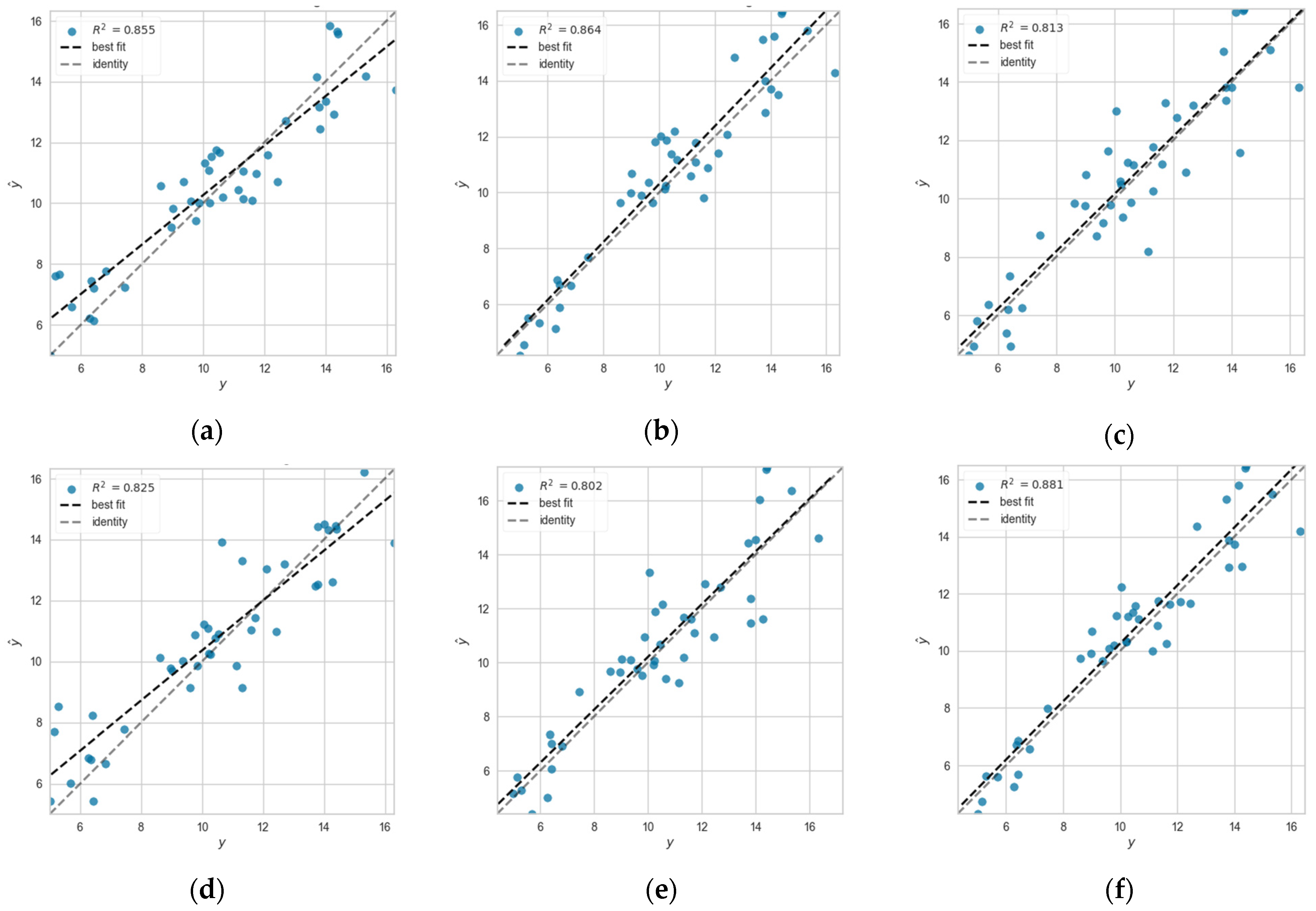
For predicting the production of the tight sand gas rate, common algorithms for regression problems were selected: random forest (RF), extremely randomized trees (ET), LightGBM (light gradient boosting machine), gradient boosting regression (GBR), and linear regression (LR). The models’ accuracy and generalization capabilities were evaluated through multiple calculations and cross-validation, resulting in the average absolute error (MAE) and mean squared error (MSE) for each model. Further model accuracy enhancement was achieved by fine-tuning the hyperparameters. The randomly generated testing set (42 wells) was used for the prediction, and the calculation results are detailed in Table 2. The accuracy of the five models for predicting the tight gas production was 0.8553, 0.8642, 0.8129, 0.8017, and 0.8251, respectively. Additionally, Q-Q plots were generated for each model to observe the deviation between the calculated and predicted values, as shown in Figure 3.

Table 2.
Comparison of prediction results for single-well production in tight gas using five different models.
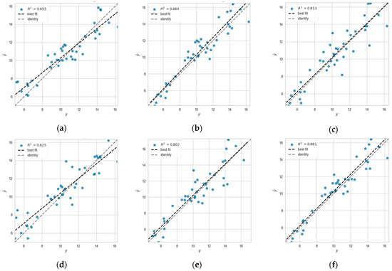
Figure 3.
Q-Q plot of the prediction results for tight gas production rate. (a) RF model, (b) ET model, (c) LightGBM model, (d) LR model, (e) GBR model, (f) Blending model.
To further improve the accuracy of the model predictions, ensemble learning was used to combine the predictions from multiple base models to enhance the model’s generalization ability and accuracy. Ensemble learning mainly includes two common methods: blending and stacking. Blending is a simple ensemble learning method that takes the predictions from multiple base models as features and inputs them into a meta-model to obtain the final predictions. Stacking is a more complex ensemble learning method that also takes the predictions from multiple base models as the features, but inputs them into one or more meta-models to obtain the final predictions. Comparatively, while stacking can use cross-validation to reduce overfitting and employ multiple layers of meta-models to increase the model’s complexity and expressive power, its implementation is complex and requires the tuning of multiple parameters, resulting in lower computational efficiency. On the other hand, blending has the advantage of simplicity, does not require cross-validation, and has a higher computational efficiency. However, it should be noted that potential overfitting should be avoided as much as possible. See Figure 4 for the computational flow.

Figure 4.
Blending process flowchart.
Using ensemble learning, the prediction results of three models, namely Random Forest, Extremely Randomized Trees, and Linear Regression, which demonstrated good performance in forecasting gas production, were used as the new features. These prediction results, combined with the original features, formed the new feature space of the blended training set. Then, an ensemble model was utilized to obtain the final prediction for tight sand gas production rate. The calculated results show that the blending model, by leveraging the advantages of multiple models, reduced the average absolute error (MAE) and mean squared error (MSE) compared to the five individual models mentioned above. The blending model achieved an MAE of 0.8419 and an MSE of 1.0930, with an R2 score of 0.8812, indicating a high predictive accuracy and reliability. The detailed results can be found in Table 3. This demonstrates the applicability of ensemble learning, specifically the blending method, for tight gas well production prediction.

Table 3.
Prediction results of the blending model for gas rate in tight gas reservoirs.
4. Production Rate Prediction in Shale Gas Field B
4.1. Overview
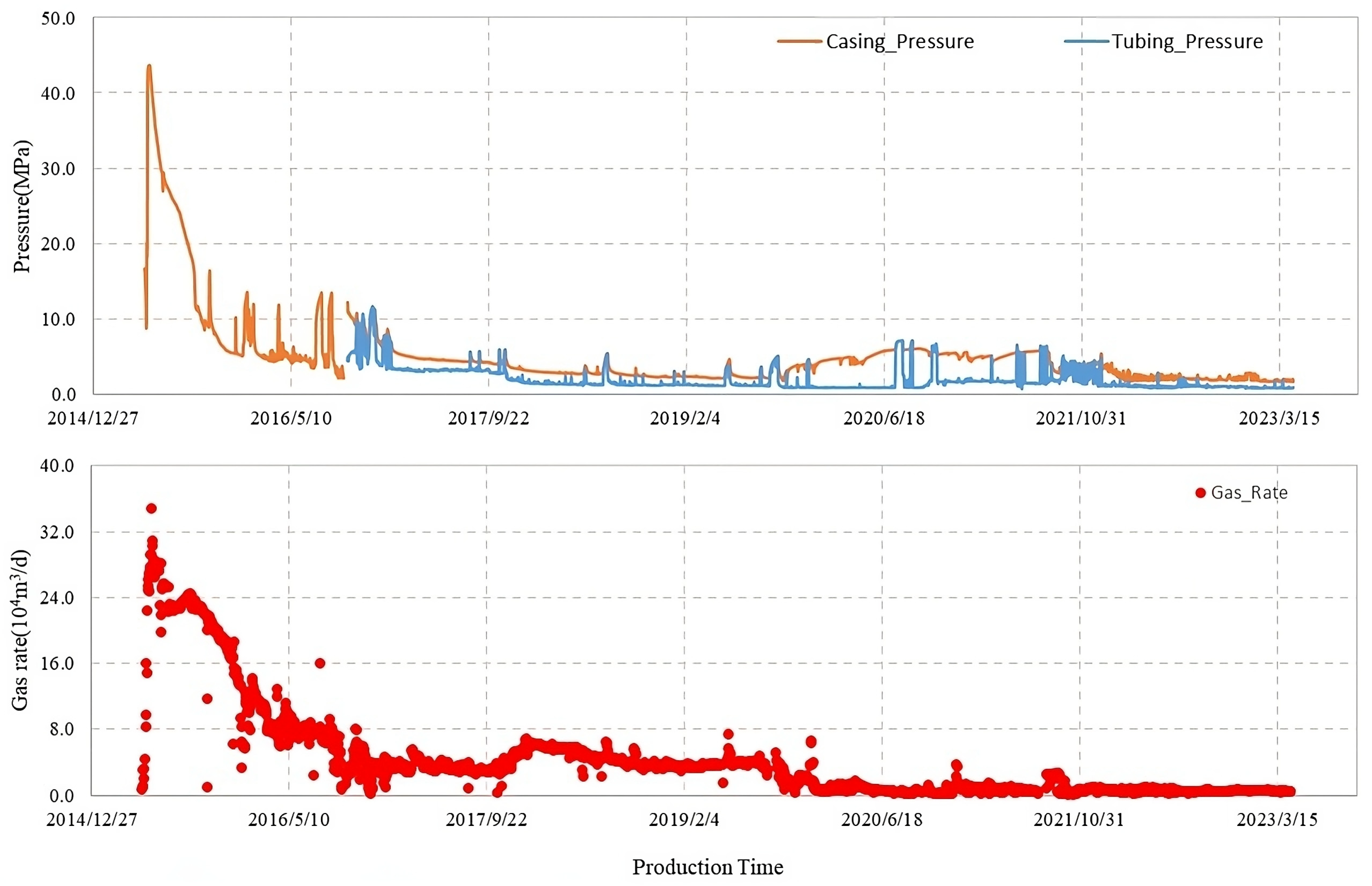
Gas Field B had a depth ranging from 8202 to 13,123 ft. The average thickness of the shale reservoir was 152.2 ft, while the average thickness of the layers was 15.1 ft. The total organic carbon (TOC) content ranged from 1.5% to 3.5%, with an average of 3.2%. The porosity ranged from 3% to 8%, with an average of 6%. The gas saturation ranged from 50% to 70%, with an average of 63%. The content of brittle minerals ranged from 65% to 87%, with an average of 74%. Horizontal wells with volume fracturing were used as the development approach to achieve complex fracture networks, increase the effective stimulation volume and fracture conductivity, and reduce the distance between the shale gas and fractures. A staged technique was used, combining bridge plugs and clustered cable perforation. The length of the fracturing sections ranged from 148 m to 361 ft, with each section having 4 to 12 clusters, and cluster spacing of 16 to 33 ft. The average sand concentration was 13,228 pounds/ft, and the average fluid intensity was 3.0 mcf/ft. The pumping capacity ranged from 0.4 mcf/min to 0.6 mcf/min. The initial production rates of the 193 wells in the study area ranged from 1.2 to 1.9 mmcf/d. Figure 5 illustrates a typical single-well production curve in the study area.
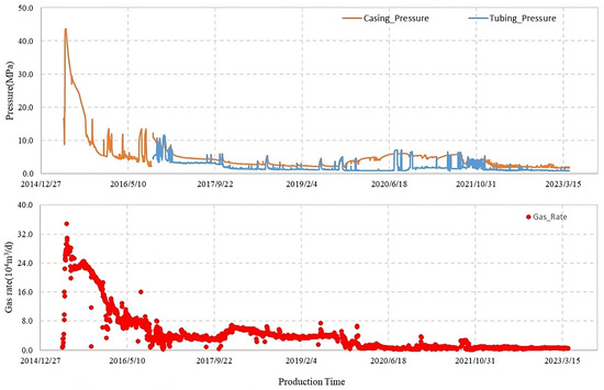
Figure 5.
Typical Production curve of deviated wells in Gas Field B.
4.2. Production Forecast
Datasets were collected from 207 wells in shale gas blocks in Gas Field B, including the geological reservoir parameters, engineering parameters, and production data, to obtain the original dataset. The original data had some missing values (1.0%) which were filled in using interpolation, and the abnormal values were processed. The dataset consisted of 37 data features. Through pairwise relationship analysis, the factors with weak correlations to the production rate were eliminated. After processing, 21 factors were identified that were correlated to the production, including sweet spot zoning, the shut-in time, the length of the horizontal section, the reservoir depth, the drilling encounter rate, the layer thickness, the single-well controlled reserves, the well spacing, the length of the fracturing reconstruction, the length of the fracturing stage, the number of fracturing stages, the fluid volume per stage, the sand volume per stage, the percentage of fine sand, the reservoir classification, and the pressure. Figure 6 analyzes the pairwise relationship between the single-well production rate of shale gas and fracture length.
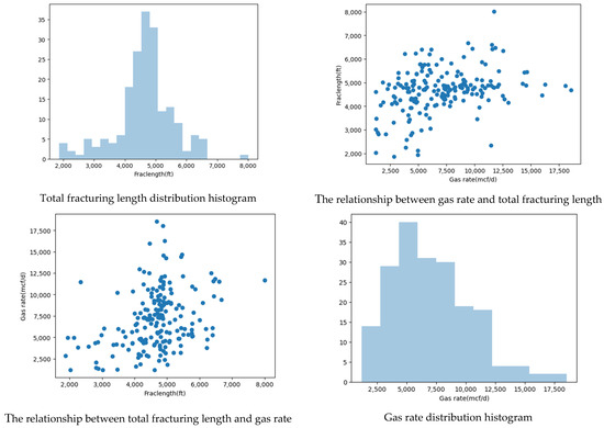
Figure 6.
Pair plot between gas rate and fracture length in shale gas reservoir.
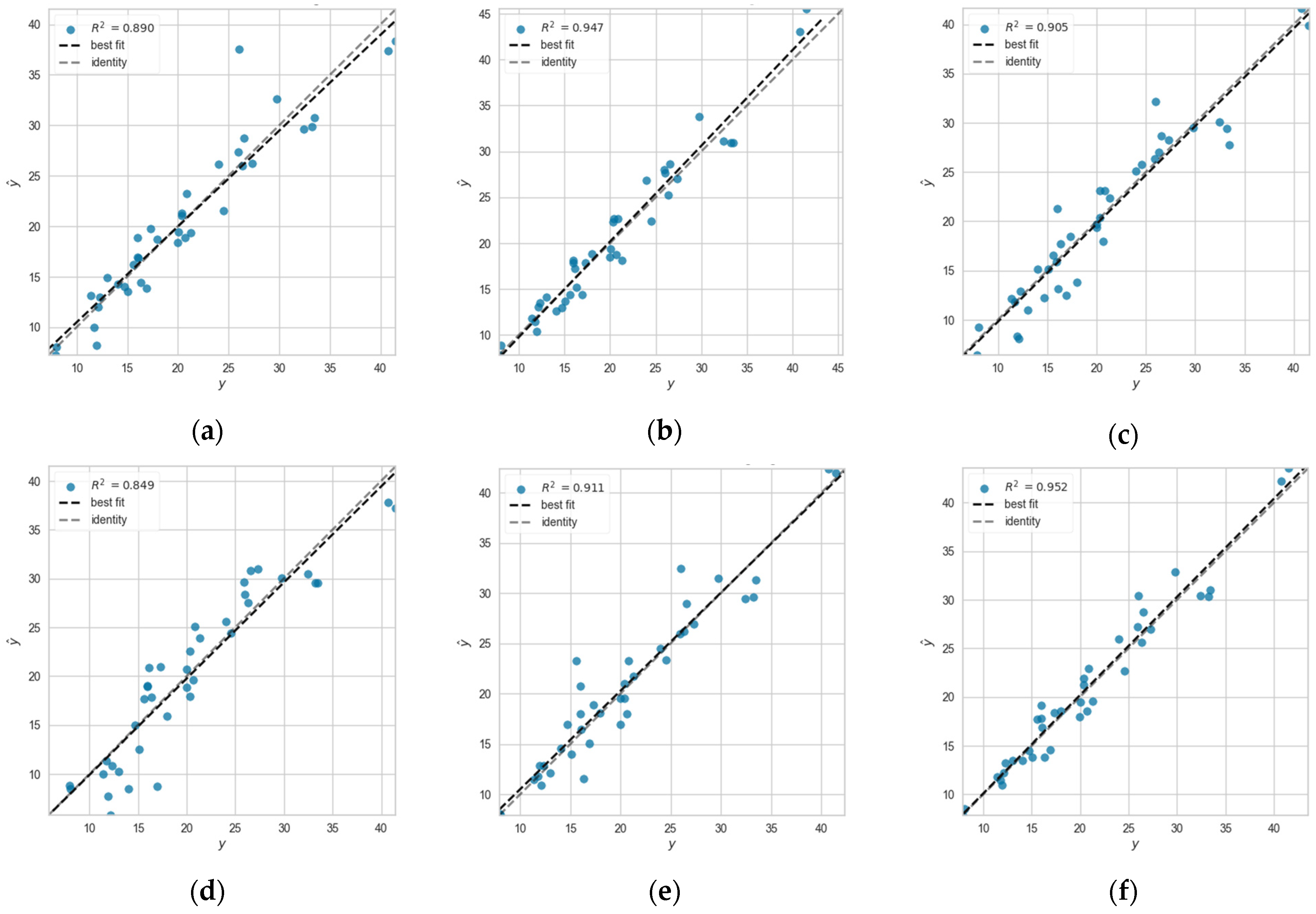
The above 21 features had different dimensions and significant differences in the numerical values among the indicators. To preprocess the data, normalization was performed on the training and testing sets, limiting the preprocessed data to the range of [0, 1]. Considering that the collected data samples consisted of 193 wells, to ensure sufficient data for the model training in the training set and an adequate amount of data to evaluate the model’s performance in the testing set, a ratio of 8:2 was used to split the dataset into the training and testing sets, with 80% of the data allocated to the training set and 20% to the testing set. In this study, random forest (RF), extremely randomized trees (ET), light gradient boosting machine (LightGBM), gradient boosting regressor (GBR), and linear regression (LR) were used for predicting the production of tight sand gas. The models’ average absolute error (MAE) and mean squared error (MSE) were obtained through multiple computations to assess the accuracy and generalization of the models using cross-validation. Further accuracy improvement was achieved by tuning the parameters of each model. Generated test data (39 wells) were fed into the models for the prediction. The accuracy rates for predicting tight gas production by applying the five models were 0.8898, 0.9468, 0.9045, 0.9109, and 0.8486, respectively. The calculation results can be found in Table 4. Similarly, Q-Q plots were created for each model to observe the deviation between the calculated values and the predicted values, as shown in Figure 7.

Table 4.
Comparison of prediction results for single-well production in shale gas using five different models.
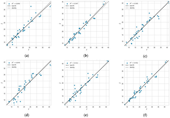
Figure 7.
Q-Q plot of the prediction results for shale gas production rate. (a) RF model, (b) ET model, (c) LightGBM model, (d) LR model, (e) GBR model, (f) blending model.
To further improve the accuracy of the model predictions, a blending ensemble learning method was adopted. The predictions of three models, namely extremely randomized trees (ET), light gradient boosting machine (LightGBM), and gradient boosting regressor (GBR), which performed well in the gas production estimation, were used as the new features. Together with the original features, these formed the new feature space of the blended training set. An ensemble model was then used to obtain the final shale gas production prediction rate. The calculation results showed that the blending model, leveraging the advantages of multiple models, achieved a reduction in the average absolute error (MAE) and mean squared error (MSE) compared to the results of the previous five models. The blending model achieved an MAE of 1.4841 and an MSE of 3.1629, with an R2 score of 0.9524, indicating a high predictive accuracy and reliability. The detailed calculation results can be found in Table 5. This demonstrates that the blending-based ensemble learning model is more applicable for predicting the shale gas well production.

Table 5.
Prediction results of the blending model for gas rate in shale gas reservoirs.
5. Conclusions and Future Work
- (1)
- This article proposes a reasonable production prediction model and method for single-well tight gas and shale gas rate based on artificial intelligence analysis. The method combines the predictions of multiple base models, such as random forest (RF), extremely randomized trees (ET), light gradient boosting machine (LightGBM), and gradient boosting regressor (GBR), and further improves the accuracy and generalization ability of the model predictions through ensemble learning.
- (2)
- The blending-based ensemble learning model has higher accuracy and reliability for predicting the single-well gas rate of unconventional reservoirs. The blending ensemble model, utilizing the advantages of multiple basic models, predicts the production of the tight gas rate, with an accuracy rate improved to 0.8812. The blending ensemble model also improves the accuracy rate for predicting the shale gas production rate to 0.9524.
- (3)
- Considering the characteristics of the multiple influencing factors and a limited number of effective samples in the gas production prediction rate, further research is planned to be conducted on the production prediction driven by data and knowledge graph integration. The temporal and spatial relationships of oil well production are represented using knowledge graphs, with graph embedding techniques employed to represent the vector feature graphs. The vector features of the knowledge graph and the features extracted via deep learning are organically fused using embedding layers to achieve an integrated prediction of the gas well production rate through the fusion of data and knowledge.
Author Contributions
Research Methodology, F.Y. and X.L.; Coding, F.Y. and F.X.; Result analysis and discussion, F.X. and F.Y.; Investigation, N.Z. and F.X.; Data Collection, N.Z.; Writing, F.Y. and F.X. All authors have read and agreed to the published version of the manuscript.
Funding
This research was funded by the China National Petroleum Corporation (CNPC)’s frontier and fundamental technology research project “Research on key artificial intelligence technologies for oil and gas exploration and development—Intelligent technology of oilfield development knowledge base (2023DJ8406)”.
Data Availability Statement
The data used in this research are confidential.
Acknowledgments
The authors would like to acknowledge China National Petroleum Corporation (CNPC)’s frontier and fundamental technology research project, and also thank all the researchers related to this paper.
Conflicts of Interest
The authors declare that this study received funding from “Research on key artificial intelligence technologies for oil and gas exploration and development—Intelligent technology of oilfield development knowledge base (2023DJ8406)”. The funder was not involved in the study design, collection, analysis, interpretation of data, the writing of this article or the decision to submit it for publication.
References
- Jia, A.; Wei, Y.; Guo, Z.; Wang, G.; Meng, D.; Huang, S. Development status and prospect of tight sandstone gas in China. Nat. Gas Ind. 2022, 42, 83–92. [Google Scholar] [CrossRef]
- Li, L.G. Development of natural gas industry in China: Review and prospect. Nat. Gas Ind. 2022, 9, 187–196. [Google Scholar] [CrossRef]
- Pan, J.P. New Progress and Outlook of China’s Oil and Gas Exploration and Development. Pet. Sci. Technol. Forum 2023, 42, 23–31. [Google Scholar]
- Guo, J.; Lu, Q.; Liu, Z.; Zeng, F.; Guo, T.; Liu, Y.; Liu, L.; Qiu, L. Concept and key technology of “multi-scale high-density” fracturing technology: A case study of tight sandstone gas reservoirs in the western Sichuan Basin. Nat. Gas Ind. 2023, 43, 67–76. [Google Scholar] [CrossRef]
- Zhang, N. Optimization of horizontal well pattern in southeast area of Su 53 block. Unconv. Oil Gas 2021, 8, 77–83. [Google Scholar]
- Chen, G.S.; Wu, J.F.; Liu, Y.; Huang, H.Y.; Zhao, S.J.; Chang, C.; Zhong, C.X. Geology-engineering integration key technologies for ten billion cubic meters of shale gas productivity construction in the southern Sichuan basin. Nat. Gas Ind. 2021, 41, 72–81. [Google Scholar]
- Gong, Y.; Gao, H.Q.; Li, X.Y. Study on the distribution characteristics of occurrence modes of shale gas in the Sichuan Basin and its periphery. Unconv. Oil Gas 2023, 10, 49–56. [Google Scholar]
- Li, Q.; Liu, J.; Wang, S.; Guo, Y.; Han, X.; Li, Q.; Cheng, Y.; Dong, Z.; Li, X.; Zhang, X. Numerical insights into factors affecting collapse behavior of horizontal wellbore in clayey silt hydrate-bearing sediments and the accompanying control strategy. Ocean Eng. 2024, 297, 117029. [Google Scholar] [CrossRef]
- Micheal, M.; Xu, W.; Jin, J.; Yu, H.; Liu, J.; Jiang, W.; Liu, H.; Wu, H. A multi-scale quadruple-continuum model for production evaluation of shale gas reservoirs considering complex gas transfer mechanisms and geomechanics. J. Pet. Sci. Eng. 2022, 213, 110419. [Google Scholar] [CrossRef]
- Wang, Y.; Li, Q.; Dong, W.; Li, Q.; Wang, F.; Bai, H.; Zhang, R.; Owusu, A.B. Effect of different factors on the yield of epoxy-terminated polydimethylsiloxane and evaluation of CO2 thickening. RSC Adv. 2018, 8, 39787–39796. [Google Scholar] [CrossRef]
- Duong, A.N. An unconventional rate decline approach for tight and fracture-dominated gas wells. In Proceedings of the Canadian Unconventional Resources and International Petroleum Conference, Calgary, AB, Canada, 19–21 October 2010. [Google Scholar]
- Zhang, N. A new method of productivity evaluation for fractured horizontal well in tight gas reservoir. Sci. Technol. Eng. 2014, 14, 76–80. [Google Scholar]
- Ye, J.W. EUR Evaluation Method for Intensive Cutting Fracturing Horizontal Wells in Tight Sandstone Reservoirs. Master’s Thesis, Chengdu University of Technology, Chengdu, China, 2021. [Google Scholar]
- Zhang, N. Classification evaluation of production dynamic for horizontal well in Su 53 block. Unconv. Oil Gas 2021, 8, 88–94. [Google Scholar]
- Song, H.; Su, Y.; Xiong, X.; Liu, Y.; Zhong, S.C.; Wang, J.J. EUR evaluation workflow and influence factors for shale gas well. Nat. Gas Geosci. 2019, 30, 1531–1537. [Google Scholar]
- Zhao, Y.L.; Liang, H.B.; Jing, C.; Shang, S.F.; Li, C.Y. A new method for quick EUR evaluation of shale gas wells. J. Southwest Pet. Univ. (Sci. Technol. Ed.) 2019, 41, 124–131. [Google Scholar]
- Ma, W.D. Productivity Regularity Research of Fractured Well in Tight Gas Reservoir. Master’s Thesis, China University of Petroleum, Beijing, China, 2015. [Google Scholar]
- Tian, Y.P.; Ju, B.S. A model for predicting shale gas production decline based on the BP neural network improved by the genetic algorithm. China Sci. Pap. 2016, 11, 1710–1715. [Google Scholar]
- Zhu, H.; Kong, D.Q.; Qian, X. Shale gas production prediction method based on adaptive threshold denoising BP neural network. Sci. Technol. Eng. 2017, 17, 128–132. [Google Scholar]
- Lu, Z.Y. Research on Production Forecast Method of Gas Well in Tight Gas Reservoir Based on Big Data Analysis. Master’s Thesis, Southwest Petroleum University, Chengdu, China, 2019. [Google Scholar]
- Ma, W.L.; Li, Z.P.; Sun, Y.P.; Zhang, J.P.; Deng, S.Z. Non-deterministic shale gas productivity forecast based on machine learning. Spec. Oil Gas Reserv. 2019, 26, 101–105. [Google Scholar]
- Fan, Y.; Huang, H.Y.; Wang, X.H.; Chen, J.; Deng, Y.C. Study on the production prediction technology for shale gas horizontal well by applying data mining. In Proceedings of the 31st National Natural Gas Academic Annual Conference, Hefei, China, 31 October–1 November 2019. [Google Scholar]
- Li, Y.Z.; Bai, Y.H.; Xu, B.X. Application of NARX model in production performance prediction of tight gas wells. In Proceedings of the International Field Exploration and Development Conference, Chengdu, China, 23–25 September 2020. [Google Scholar]
- Chen, J.; Huang, H.Y.; Liu, J.C.; Zeng, B.; Yang, X.R. Production predicting technology of shale gas fracturing Horizontal well in changning area based on the GA-BP neural network mode. Sci. Technol. Eng. 2020, 20, 1851–1858. [Google Scholar]
- Zhao, Q.Y.; Liu, Y.; Liu, L.P.; Chen, H.; Ning, M.; Liu, J.; Gao, W.B.; Miao, R.J. Application of machine learning in the production prediction of horizontal wells in tight gas reservoirs. In Proceedings of the 17th Ningxia Young Scientists Forum Petroleum and Petrochemical Special Forum, Yinchuan, China, 15 September 2021. [Google Scholar]
- Yan, Z.M.; Wang, T.; Liu, Z.L.; Zhuang, Z. Machine-learning-based prediction methods on shale gas recovery. Chin. J. Solid Mech. 2021, 42, 221–232. [Google Scholar]
- He, Y.W.; He, Z.Y.; Tang, Y.; Qin, J.Z.; Song, J.J.; Wang, Y. Shale gas well production evaluation and prediction based on machine learning. Oil Drill. Prod. Technol. 2021, 43, 518–524. [Google Scholar]
- Otchere, D.A.; Ganat, O.T.; Gholami, R.; Lawal, M. A Novel Custom Ensemble Learning Model for an Improved Reservoir Permeability and Water Saturation Prediction. J. Nat. Gas Sci. Eng. 2021, 91, 103962. [Google Scholar] [CrossRef]
- Niu, W.; Lu, J.; Sun, Y. Development of shale gas production prediction models based on machine learning using early data. Energy Rep. 2022, 8, 1229–1237. [Google Scholar] [CrossRef]
- Wang, H.; Qiao, L.; Lu, S.; Chen, F.; Fang, Z.; He, X.; Zhang, J.; He, T. A novel shale gas production prediction model based on machine learning and its application in optimization of multistage fractured horizontal wells. Front. Earth Sci. 2021, 9, 726537. [Google Scholar] [CrossRef]
- Syed, F.I.; Alnaqbi, S.; Muther, T.; Dahaghi, A.K.; Negahban, S. Smart shale gas production performance analysis using machine learning applications. Pet. Explor. Dev. 2022, 49, 21–31. [Google Scholar] [CrossRef]
- Liao, L.; Li, G.; Zhang, H.; Feng, J.; Zeng, Y.; Ke, K.; Wang, Z. Well completion optimization in Canada tight gas fields using ensemble machine learning. In Proceedings of the Abu Dhabi International Petroleum Exhibition & Conference, Abu Dhabi, United Arab Emirates, 9–12 November 2020. [Google Scholar]
Disclaimer/Publisher’s Note: The statements, opinions and data contained in all publications are solely those of the individual author(s) and contributor(s) and not of MDPI and/or the editor(s). MDPI and/or the editor(s) disclaim responsibility for any injury to people or property resulting from any ideas, methods, instructions or products referred to in the content. |
© 2024 by the authors. Licensee MDPI, Basel, Switzerland. This article is an open access article distributed under the terms and conditions of the Creative Commons Attribution (CC BY) license (https://creativecommons.org/licenses/by/4.0/).

