
Improved Dujiangyan Irrigation System Optimization (IDISO): A Novel Metaheuristic Algorithm for Hydrochar Characteristics

 ,
,
Abstract
1. Introduction
- We improved the Dujiangyan irrigation system optimization (DISO) by introducing nonlinear shrinking factors and the Cauchy mutation mechanism, addressing its tendency to become trapped in local optima and its poor performance in high-dimensional spaces.
- We compared the IDISO algorithm with seventeen state-of-the-art optimization algorithms using twenty-nine CEC2017 benchmark functions across three dimensions (30, 50, and 100) and nine engineering problems. Non-parametric tests indicated that the IDISO algorithm showed significant improvements in terms of convergence speed and accuracy.
- We developed an IDISO-XGBoost model to predict the physicochemical properties of hydrochar, resulting in a prediction model with high robustness and generalization ability.
2. Materials and Methods
2.1. Data Source
2.2. DISO
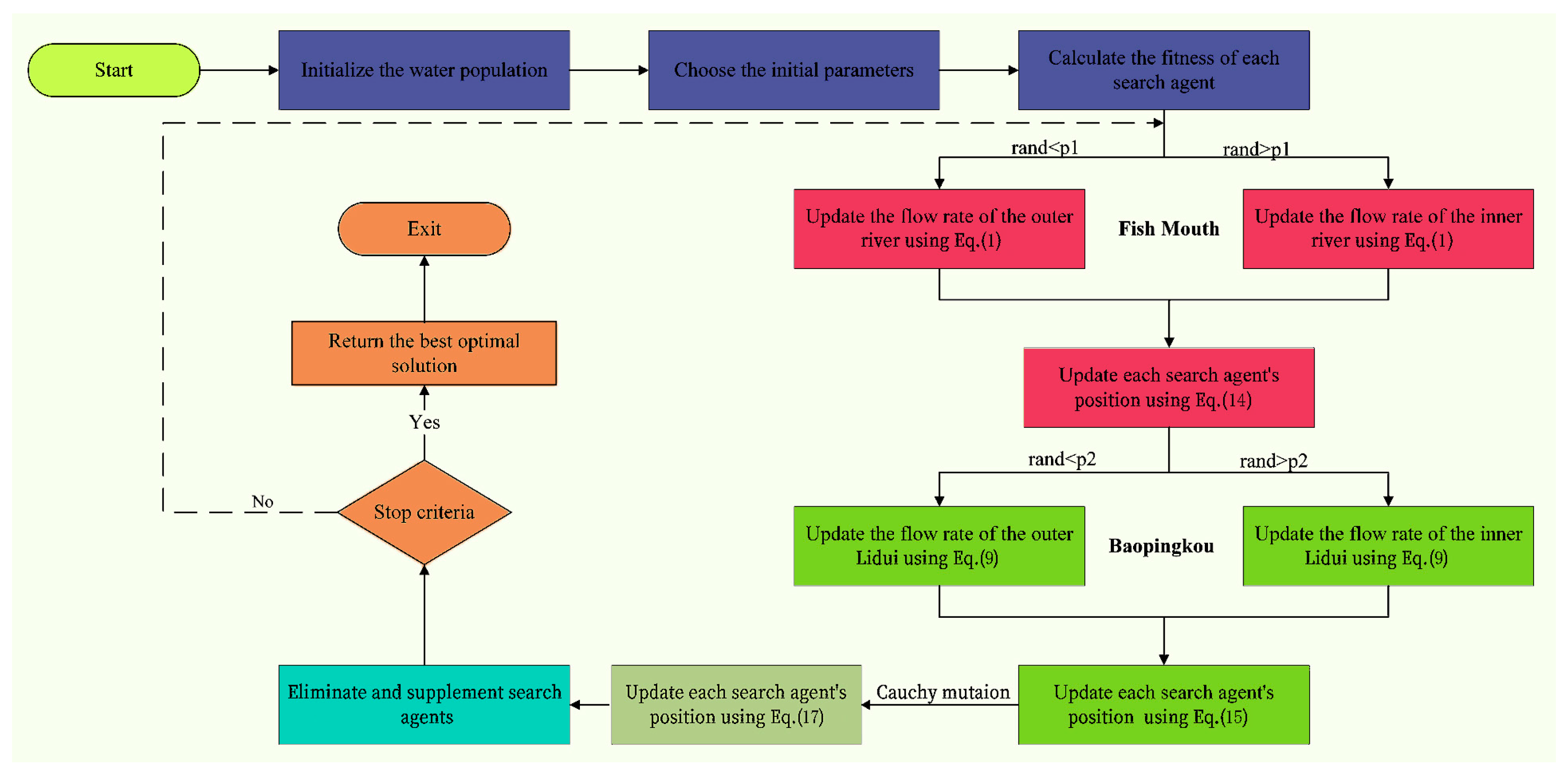
2.3. IDISO
2.3.1. Nonlinear Shrinking Factor
2.3.2. Cauchy Mutation Mechanism
2.4. IDISO-XGBoost
2.5. Performance Evaluation
2.5.1. Statistical Analysis
2.5.2. Non-parametric Statistics (Sign Test)
3. CEC2017 Results and Discussion
4. Real-World Engineering Problem Results and Discussion
5. IDISO Algorithm Analysis
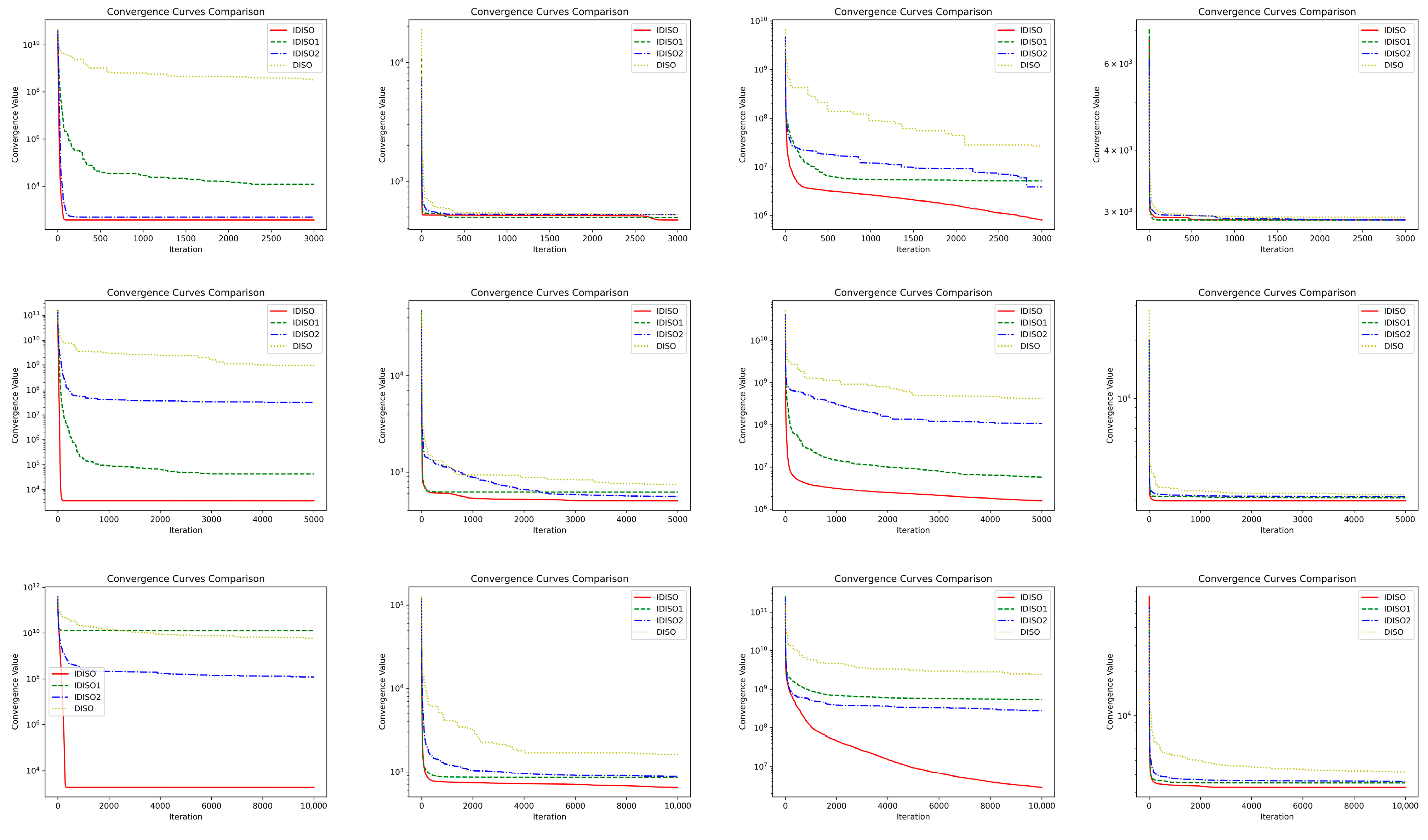
5.1. Convergence Analysis
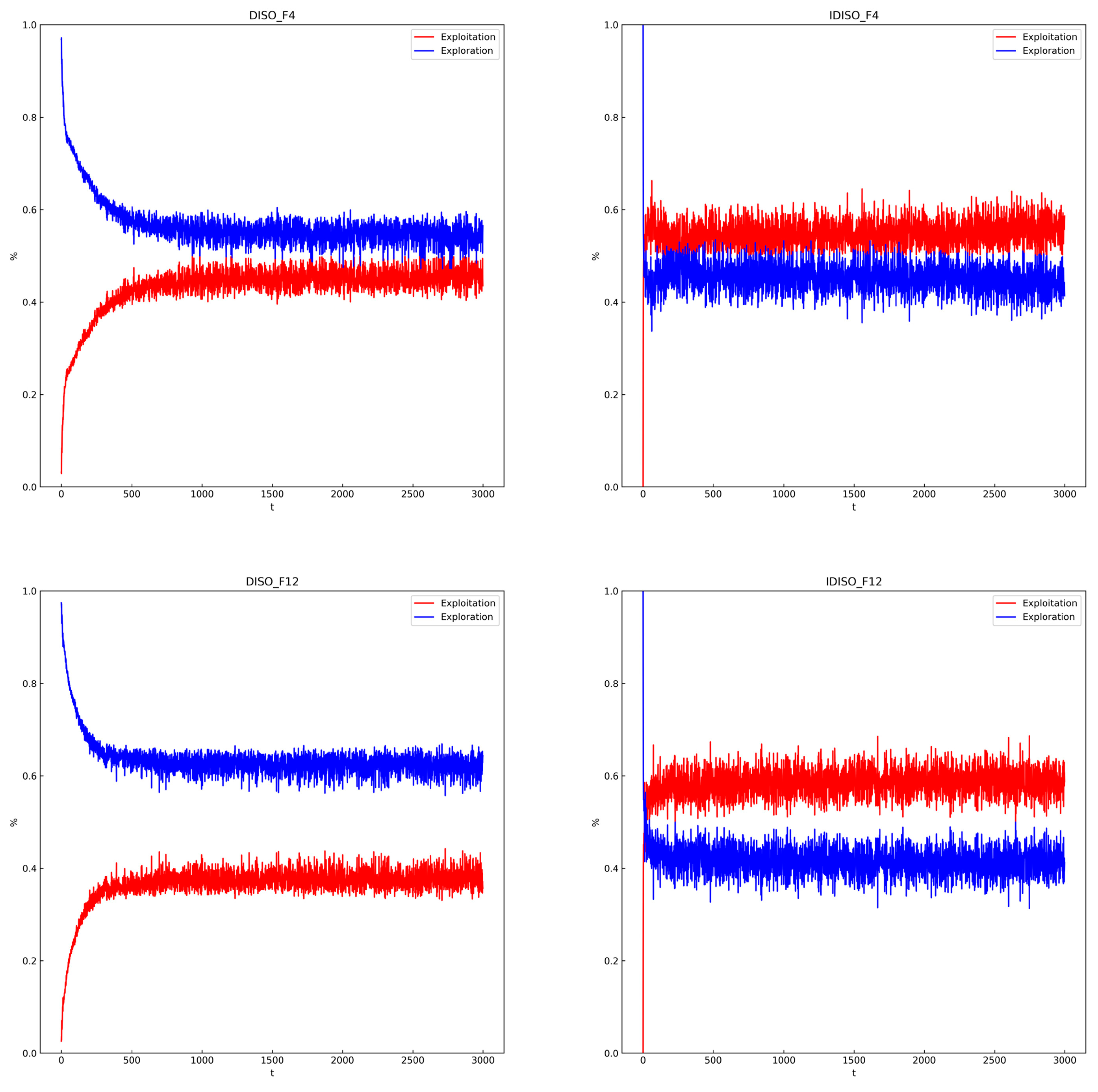
5.2. Exploration and Exploitation Analysis
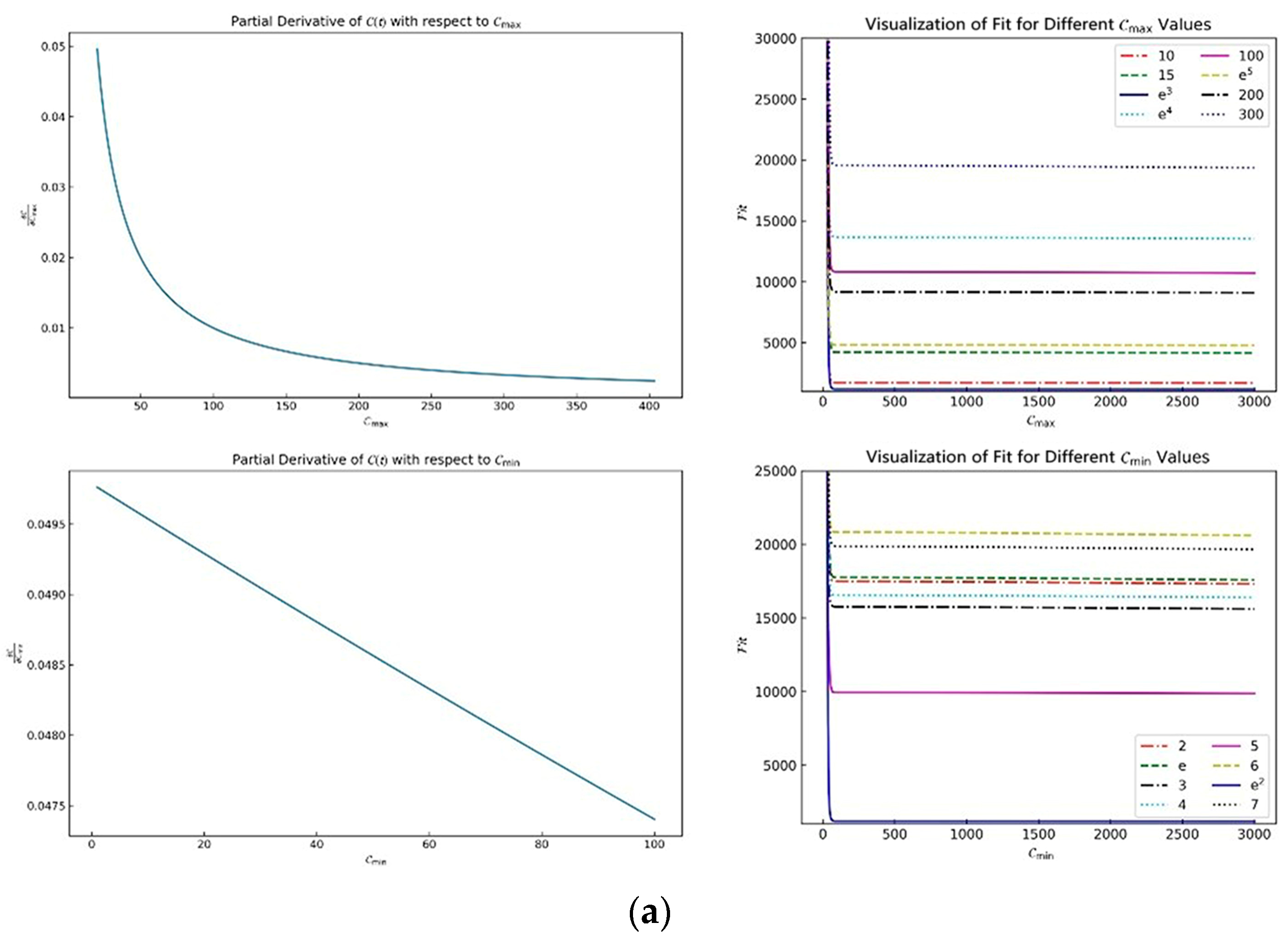
5.3. Parameter Sensitivity Analysis
5.4. IDISO Complexity Analysis
5.5. IDISO Ablation Study
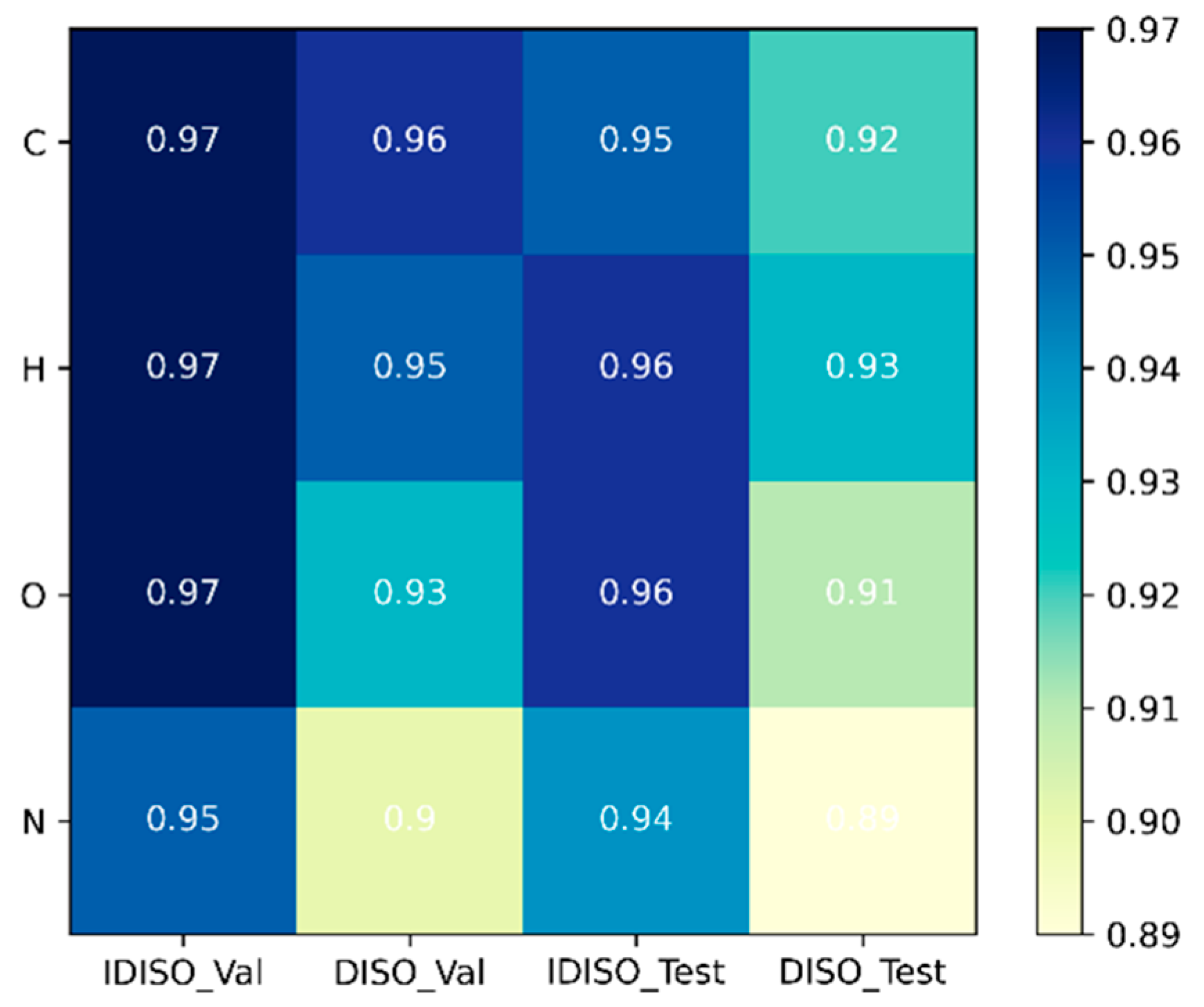
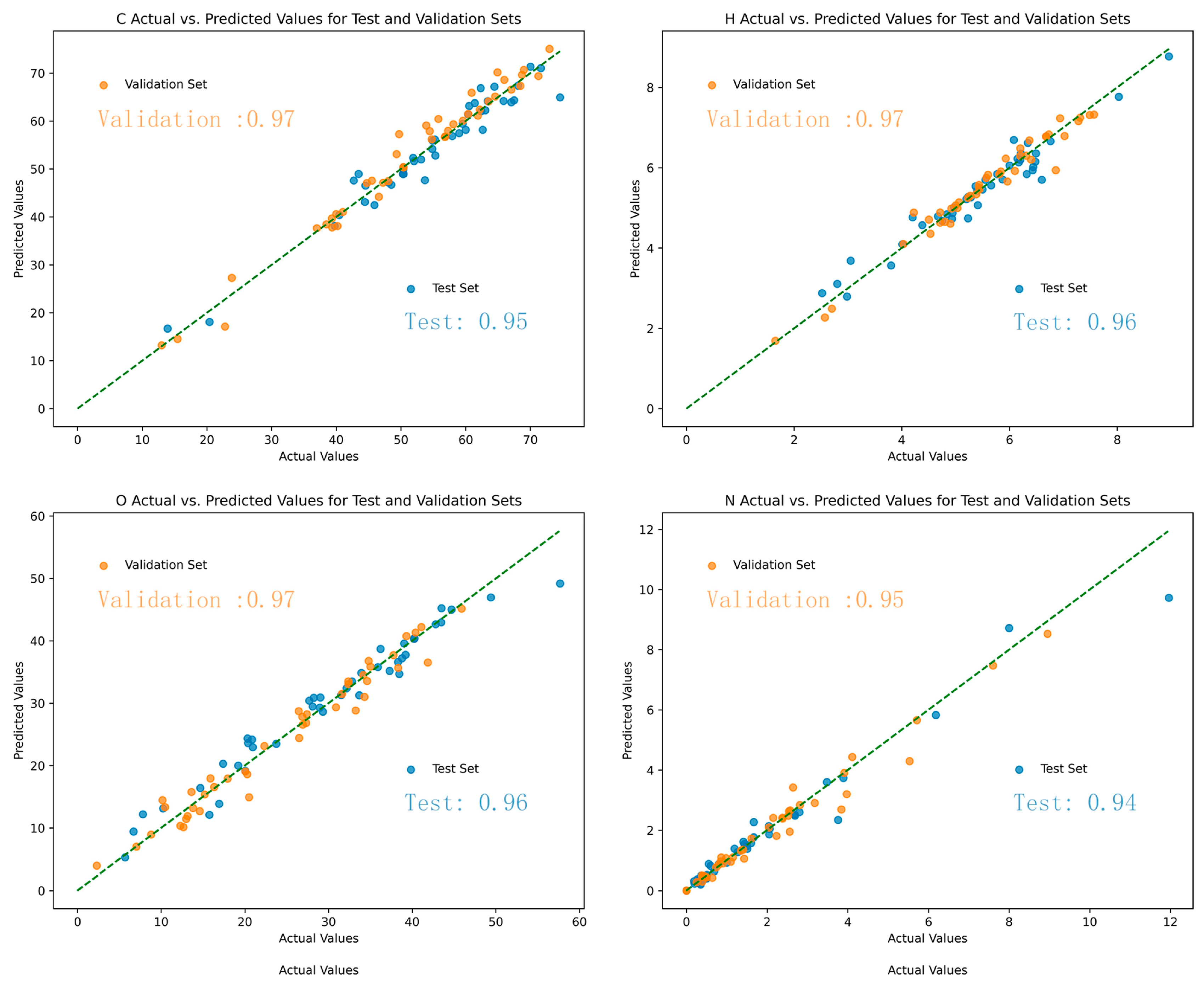
6. IDISO-XGBoost Model
7. Conclusions
Supplementary Materials
Author Contributions
Funding
Data Availability Statement
Acknowledgments
Conflicts of Interest
References
- Xiu, S.; Shahbazi, A. Bio-oil production and upgrading research: A review. Renew. Sustain. Energy Rev. 2012, 16, 4406–4414. [Google Scholar] [CrossRef]
- Lee, D.; Nam, H.; Seo, M.W.; Lee, S.H.; Tokmurzin, D.; Wang, S.; Park, Y.-K. Recent progress in the catalytic thermochemical conversion process of biomass for biofuels. Chem. Eng. J. 2022, 447, 137501. [Google Scholar] [CrossRef]
- Sikarwar, V.S.; Zhao, M.; Fennell, P.S.; Shah, N.; Anthony, E.J. Progress in biofuel production from gasification. Prog. Energy Combust. Sci. 2017, 61, 189–248. [Google Scholar] [CrossRef]
- Mäkelä, M.; Benavente, V.; Fullana, A. Hydrothermal carbonization of industrial mixed sludge from a pulp and paper mill. Bioresour. Technol. 2016, 200, 444–450. [Google Scholar] [CrossRef] [PubMed]
- Hansen, L.J.; Fendt, S.; Spliethoff, H. Impact of hydrothermal carbonization on combustion properties of residual biomass. Biomass Convers. Biorefinery 2022, 12, 2541–2552. [Google Scholar] [CrossRef]
- Samaksaman, U.; Pattaraprakorn, W.; Neramittagapong, A.; Kanchanatip, E. Solid fuel production from macadamia nut shell: Effect of hydrothermal carbonization conditions on fuel characteristics. Biomass Convers. Biorefinery 2021, 13, 2225–2232. [Google Scholar] [CrossRef]
- Wong, K.I.; Wong, P.K.; Cheung, C.S.; Vong, C.M. Modelling of diesel engine performance using advanced machine learning methods under scarce and exponential data set. Appl. Soft Comput. 2013, 13, 4428–4441. [Google Scholar] [CrossRef]
- Jeon, P.R.; Moon, J.-H.; Olanrewaju, O.N.; Lee, S.H.; Ling, J.L.J.; You, S.; Park, Y.-K. Recent advances and future prospects of thermochemical biofuel conversion processes with machine learning. Chem. Eng. J. 2023, 471, 144503. [Google Scholar] [CrossRef]
- Rasam, S.; Talebkeikhah, F.; Talebkeikhah, M.; Salimi, A.; Moraveji, M.K. Physico-chemical properties prediction of hydrochar in macroalgae Sargassum horneri hydrothermal carbonisation. Int. J. Environ. Anal. Chem. 2021, 101, 2297–2318. [Google Scholar] [CrossRef]
- Kardani, N.; Hedayati Marzbali, M.; Shah, K.; Zhou, A. Machine learning prediction of the conversion of lignocellulosic biomass during hydrothermal carbonization. Biofuels 2022, 13, 703–715. [Google Scholar] [CrossRef]
- Li, J.; Pan, L.; Suvarna, M.; Tong, Y.W.; Wang, X. Fuel properties of hydrochar and pyrochar: Prediction and exploration with machine learning. Appl. Energy 2020, 269, 115166. [Google Scholar] [CrossRef]
- Li, J.; Zhu, X.; Li, Y.; Tong, Y.W.; Ok, Y.S.; Wang, X. Multi-task prediction and optimization of hydrochar properties from high-moisture municipal solid waste: Application of machine learning on waste-to-resource. J. Clean. Prod. 2021, 278, 123928. [Google Scholar] [CrossRef]
- Nguyen, V.G.; Sharma, P.; Ağbulut, Ü.; Le, H.S.; Tran, V.D.; Cao, D.N. Precise prognostics of biochar yield from various biomass sources by Bayesian approach with supervised machine learning and ensemble methods. Int. J. Green Energy 2023, 21, 2180–2204. [Google Scholar] [CrossRef]
- Mu, L.; Wang, Z.; Wu, D.; Zhao, L.; Yin, H. Prediction and evaluation of fuel properties of hydrochar from waste solid biomass: Machine learning algorithm based on proposed PSO–NN model. Fuel 2022, 318, 123644. [Google Scholar] [CrossRef]
- Li, P.; Du, Z.; Chang, C.; Zhao, S.; Xu, G.; Xu, C.C. Efficient catalytic conversion of waste peanut shells into liquid biofuel: An artificial intelligence approach. Energy Fuels 2020, 34, 1791–1801. [Google Scholar] [CrossRef]
- Osaba, E.; Villar-Rodriguez, E.; Del Ser, J.; Nebro, A.J.; Molina, D.; LaTorre, A.; Suganthan, P.N.; Coello, C.A.C.; Herrera, F. A tutorial on the design, experimentation and application of metaheuristic algorithms to real-world optimization problems. Swarm Evol. Comput. 2021, 64, 100888. [Google Scholar] [CrossRef]
- Gavrilas, M. Heuristic and metaheuristic optimization techniques with application to power systems. In Proceedings of the 12th WSEAS International Conference on Mathematical Methods and Computational Techniques in Electrical Engineering, Kantaoui, Sousse, Tunisia, 3–6 May 2010; pp. 95–103. [Google Scholar]
- Abualigah, L.; Elaziz, M.A.; Khasawneh, A.M.; Alshinwan, M.; Ibrahim, R.A.; Al-Qaness, M.A.; Mirjalili, S.; Sumari, P.; Gandomi, A.H. Meta-heuristic optimization algorithms for solving real-world mechanical engineering design problems: A comprehensive survey, applications, comparative analysis, and results. Neural Comput. Appl. 2022, 34, 4081–4110. [Google Scholar] [CrossRef]
- Houssein, E.H.; Hosney, M.E.; Oliva, D.; Mohamed, W.M.; Hassaballah, M. A novel hybrid Harris hawks optimization and support vector machines for drug design and discovery. Comput. Chem. Eng. 2020, 133, 106656. [Google Scholar] [CrossRef]
- Turgut, O.E.; Turgut, M.S.; Kırtepe, E. A systematic review of the emerging metaheuristic algorithms on solving complex optimization problems. Neural Comput. Appl. 2023, 35, 14275–14378. [Google Scholar] [CrossRef]
- Niu, J.; Ren, C.; Guan, Z.; Cao, Z. Dujiangyan irrigation system optimization (DISO): A novel metaheuristic algorithm for dam safety monitoring. Structures 2023, 54, 399–419. [Google Scholar] [CrossRef]
- Blackwell, T.; Kennedy, J.; Poli, R. Particle swarm optimization. Swarm Intell. 2007, 1, 33–57. [Google Scholar]
- Chen, C.; Liang, R.; Wang, J.; Ge, Y.; Tao, J.; Yan, B.; Chen, G. Simulation and optimization of co-pyrolysis biochar using data enhanced interpretable machine learning and particle swarm algorithm. Biomass Bioenergy 2024, 182, 107111. [Google Scholar] [CrossRef]
- Mirjalili, S.; Mirjalili, S.; Lewis, A. Grey wolf optimizer. Adv. Eng. Softw. 2014, 69, 46–61. [Google Scholar] [CrossRef]
- Subudhi, U.; Dash, S. Detection and classification of power quality disturbances using GWO ELM. J. Ind. Inf. Integr. 2021, 22, 100204. [Google Scholar] [CrossRef]
- Zhao, S.; Zhang, T.; Ma, S.; Chen, M. Dandelion Optimizer: A nature-inspired metaheuristic algorithm for engineering applications. Eng. Appl. Artif. Intell. 2022, 114, 105075. [Google Scholar] [CrossRef]
- Saglam, M.; Bektas, Y.; Karaman, O.A. Dandelion Optimizer and Gold Rush Optimizer Algorithm-Based Optimization of Multilevel Inverters. Arab. J. Sci. Eng. 2024, 49, 7029–7052. [Google Scholar] [CrossRef]
- Chou, J.-S.; Molla, A. Recent advances in use of bio-inspired jellyfish search algorithm for solving optimization problems. Sci. Rep. 2022, 12, 19157. [Google Scholar] [CrossRef]
- Gouda, E.A.; Kotb, M.F.; El-Fergany, A.A. Jellyfish search algorithm for extracting unknown parameters of PEM fuel cell models: Steady-state performance and analysis. Energy 2021, 221, 119836. [Google Scholar] [CrossRef]
- Abdel-Basset, M.; El-Shahat, D.; Jameel, M.; Abouhawwash, M. Young’s double-slit experiment optimizer: A novel metaheuristic optimization algorithm for global and constraint optimization problems. Comput. Methods Appl. Mech. Eng. 2023, 403, 115652. [Google Scholar] [CrossRef]
- Dong, Y.; Sun, Y.; Liu, Z.; Du, Z.; Wang, J. Predicting dissolved oxygen level using Young’s double-slit experiment optimizer-based weighting model. J. Environ. Manag. 2024, 351, 119807. [Google Scholar] [CrossRef]
- Zamani, H.; Nadimi-Shahraki, M.H.; Gandomi, A.H. Starling murmuration optimizer: A novel bio-inspired algorithm for global and engineering optimization. Comput. Methods Appl. Mech. Eng. 2022, 392, 114616. [Google Scholar] [CrossRef]
- Chao, X. Optimal boosting method of HPC concrete compressive and tensile strength prediction. Struct. Concr. 2024, 25, 283–302. [Google Scholar] [CrossRef]
- Wolpert, D.H.; Macready, W.G. No free lunch theorems for optimization. IEEE Trans. Evol. Comput. 1997, 1, 67–82. [Google Scholar] [CrossRef]
- Laskar, N.M.; Guha, K.; Chatterjee, I.; Chanda, S.; Baishnab, K.L.; Paul, P.K. HWPSO: A new hybrid whale-particle swarm optimization algorithm and its application in electronic design optimization problems. Appl. Intell. 2019, 49, 265–291. [Google Scholar] [CrossRef]
- Hu, G.; Zheng, Y.; Abualigah, L.; Hussien, A.G. DETDO: An adaptive hybrid dandelion optimizer for engineering optimization. Adv. Eng. Inform. 2023, 57, 102004. [Google Scholar] [CrossRef]
- Hu, G.; Guo, Y.; Zhong, J.; Wei, G. IYDSE: Ameliorated Young’s double-slit experiment optimizer for applied mechanics and engineering. Comput. Methods Appl. Mech. Eng. 2023, 412, 116062. [Google Scholar] [CrossRef]
- Hu, G.; Wang, J.; Li, M.; Hussien, A.G.; Abbas, M. EJS: Multi-strategy enhanced jellyfish search algorithm for engineering applications. Mathematics 2023, 11, 851. [Google Scholar] [CrossRef]
- Hu, G.; Zhong, J.; Wei, G.; Chang, C.-T. DTCSMO: An efficient hybrid starling murmuration optimizer for engineering applications. Comput. Methods Appl. Mech. Eng. 2023, 405, 115878. [Google Scholar] [CrossRef]
- Guan, Z.; Ren, C.; Niu, J.; Wang, P.; Shang, Y. Great Wall Construction Algorithm: A novel meta-heuristic algorithm for engineer problems. Expert Syst. Appl. 2023, 233, 120905. [Google Scholar] [CrossRef]
- Chen, T.; He, T.; Benesty, M.; Khotilovich, V.; Tang, Y.; Cho, H.; Chen, K.; Mitchell, R.; Cano, I.; Zhou, T. Xgboost: Extreme gradient boosting. R Package Version 0.4-2 2015, 1, 1–4. [Google Scholar]
- Grinsztajn, L.; Oyallon, E.; Varoquaux, G. Why do tree-based models still outperform deep learning on typical tabular data? Adv. Neural Inf. Process. Syst. 2022, 35, 507–520. [Google Scholar]
- Mohamed, A.W.; Hadi, A.A.; Fattouh, A.M.; Jambi, K.M. LSHADE with semi-parameter adaptation hybrid with CMA-ES for solving CEC 2017 benchmark problems. In Proceedings of the 2017 IEEE Congress on Evolutionary Computation (CEC), Donostia, Spain, 5–8 June 2017; pp. 145–152. [Google Scholar]
- Hashim, F.A.; Hussain, K.; Houssein, E.H.; Mabrouk, M.S.; Al-Atabany, W. Archimedes optimization algorithm: A new metaheuristic algorithm for solving optimization problems. Appl. Intell. 2021, 51, 1531–1551. [Google Scholar] [CrossRef]
- Hayyolalam, V.; Kazem, A.A.P. Black widow optimization algorithm: A novel meta-heuristic approach for solving engineering optimization problems. Eng. Appl. Artif. Intell. 2020, 87, 103249. [Google Scholar] [CrossRef]
- Bairwa, A.K.; Joshi, S.; Singh, D. Dingo optimizer: A nature-inspired metaheuristic approach for engineering problems. Math. Probl. Eng. 2021, 2021, 2571863. [Google Scholar] [CrossRef]
- Ghafil, H.N.; Jármai, K. Dynamic differential annealed optimization: New metaheuristic optimization algorithm for engineering applications. Appl. Soft Comput. 2020, 93, 106392. [Google Scholar] [CrossRef]
- Heidari, A.A.; Mirjalili, S.; Faris, H.; Aljarah, I.; Mafarja, M.; Chen, H. Harris hawks optimization: Algorithm and applications. Future Gener. Comput. Syst. 2019, 97, 849–872. [Google Scholar] [CrossRef]
- Peraza-Vázquez, H.; Peña-Delgado, A.; Ranjan, P.; Barde, C.; Choubey, A.; Morales-Cepeda, A.B. A bio-inspired method for mathematical optimization inspired by arachnida salticidade. Mathematics 2021, 10, 102. [Google Scholar] [CrossRef]
- Abualigah, L.; Abd Elaziz, M.; Sumari, P.; Geem, Z.W.; Gandomi, A.H. Reptile Search Algorithm (RSA): A nature-inspired meta-heuristic optimizer. Expert Syst. Appl. 2022, 191, 116158. [Google Scholar] [CrossRef]
- Dhiman, G.; Garg, M.; Nagar, A.; Kumar, V.; Dehghani, M. A novel algorithm for global optimization: Rat swarm optimizer. J. Ambient Intell. Humaniz. Comput. 2021, 12, 8457–8482. [Google Scholar] [CrossRef]
- Mirjalili, S. SCA: A sine cosine algorithm for solving optimization problems. Knowl. -Based Syst. 2016, 96, 120–133. [Google Scholar] [CrossRef]
- Shadravan, S.; Naji, H.R.; Bardsiri, V.K. The Sailfish Optimizer: A novel nature-inspired metaheuristic algorithm for solving constrained engineering optimization problems. Eng. Appl. Artif. Intell. 2019, 80, 20–34. [Google Scholar] [CrossRef]
- Givi, H.; Hubalovska, M. Skill Optimization Algorithm: A New Human-Based Metaheuristic Technique. Comput. Mater. Contin. 2023, 74, 179–202. [Google Scholar] [CrossRef]
- Zhao, W.; Wang, L.; Zhang, Z. Supply-demand-based optimization: A novel economics-inspired algorithm for global optimization. IEEE Access 2019, 7, 73182–73206. [Google Scholar] [CrossRef]
- Dhiman, G.; Kumar, V. Spotted hyena optimizer: A novel bio-inspired based metaheuristic technique for engineering applications. Adv. Eng. Softw. 2017, 114, 48–70. [Google Scholar] [CrossRef]
- Kaur, S.; Awasthi, L.K.; Sangal, A.; Dhiman, G. Tunicate Swarm Algorithm: A new bio-inspired based metaheuristic paradigm for global optimization. Eng. Appl. Artif. Intell. 2020, 90, 103541. [Google Scholar] [CrossRef]
- Qais, M.H.; Hasanien, H.M.; Alghuwainem, S. Transient search optimization: A new meta-heuristic optimization algorithm. Appl. Intell. 2020, 50, 3926–3941. [Google Scholar] [CrossRef]
- Talatahari, S.; Bayzidi, H.; Saraee, M. Social network search for global optimization. IEEE Access 2021, 9, 92815–92863. [Google Scholar] [CrossRef]
- Hussain, K.; Salleh, M.N.M.; Cheng, S.; Shi, Y. On the exploration and exploitation in popular swarm-based metaheuristic algorithms. Neural Comput. Appl. 2019, 31, 7665–7683. [Google Scholar] [CrossRef]


| Function Classification | Function Name | Optimal Value |
|---|---|---|
| Unimodal Function | Shifted and Rotated Bent Cigar Function (F1) | 100 |
| Shifted and Rotated Zakharov Function (F3) | 300 | |
| Multimodal Function | Shifted and Rotated Rosenbrock’s Function (F4) | 400 |
| Shifted and Rotated Rastrigin’s Function (F5) | 500 | |
| Shifted and Rotated Expanded Scaffer’s F6 Function (F6) | 600 | |
| Shifted and Rotated Lunacek Bi_Rastrigin Function (F7) | 700 | |
| Shifted and Rotated Non-Continuous Rastrigin’s Function (F8) | 800 | |
| Shifted and Rotated Levy Function (F9) | 900 | |
| Shifted and Rotated Schwefel’s Function (F10) | 1000 | |
| Hybrid Function | Hybrid Function 1 (N = 3) (F11) | 1100 |
| Hybrid Function 2 (N = 3) (F12) | 1200 | |
| Hybrid Function 3 (N = 3) (F13) | 1300 | |
| Hybrid Function 4 (N = 4) (F14) | 1400 | |
| Hybrid Function 5 (N = 4) (F15) | 1500 | |
| Hybrid Function 6 (N = 4) (F16) | 1600 | |
| Hybrid Function 6 (N = 5) (F17) | 1700 | |
| Hybrid Function 6 (N = 5) (F18) | 1800 | |
| Hybrid Function 6 (N = 5) (F19) | 1900 | |
| Hybrid Function 6 (N = 6) (F20) | 2000 | |
| Composite Function | Composition Function 1 (N = 3) (F21) | 2100 |
| Composition Function 2 (N = 3) (F22) | 2200 | |
| Composition Function 3 (N = 4) (F23) | 2300 | |
| Composition Function 4 (N = 4) (F24) | 2400 | |
| Composition Function 5 (N = 5) (F25) | 2500 | |
| Composition Function 6 (N = 5) (F26) | 2600 | |
| Composition Function 7 (N = 6) (F27) | 2700 | |
| Composition Function 8 (N = 6) (F28) | 2800 | |
| Composition Function 9 (N = 3) (F29) | 2900 | |
| Composition Function 10 (N = 3) (F30) | 3000 | |
| Search Range: | ||
| Algorithm Name | Parameters |
|---|---|
| Arithmetic Optimization Algorithm (AOA) [44] | |
| Black Widow Optimization Algorithm (BWOA) [45] | |
| Dingo Optimization Algorithm (DOA) [46] | |
| Dynamic Differential Annealed Optimization (DDAO) [47] | |
| Grey Wolf Optimizer (GWO) [24] | None |
| HarrisHawk Optimization (HHO) [48] | |
| Jumping Spider Optimization Algorithm (JSOA) [49] | |
| Reptile Search Algorithm (RSA) [50] | |
| Rat Swarm Optimizer (RSO) [51] | |
| Sine Cosine Algorithm (SCA) [52] | |
| Sailfish Optimization Algorithm (SFO) [53] | |
| Skill optimization algorithm (SOA) [54] | None |
| Supply–Demand-Based Optimization (SDO) [55] | None |
| Spotted Hyena Optimizer (SHO) [56] | None |
| Tunicate Swarm Algorithm (TSA) [57] | |
| Transient search algorithm (TSO) [58] | |
| Dujiangyan irrigation system optimization (DISO) [21] |
| (a) | ||||||||||||
| Algorithm | Average D = 30 | Final D = 30 | Average D = 50 | Final D = 50 | Average D = 100 | Final D = 100 | ||||||
| IDISO | 2.41 | 1 | 2.17 | 1 | 2.06 | 1 | ||||||
| DISO | 3.37 | 3 | 3.55 | 4 | 3.62 | 4 | ||||||
| AOA | 9.51 | 9 | 10.10 | 11 | 11.44 | 11 | ||||||
| BWOA | 8.65 | 8 | 9.62 | 9 | 10.72 | 10 | ||||||
| DOA | 5.37 | 5 | 5.93 | 5 | 7.13 | 7 | ||||||
| DDOA | 11 | 12 | 11.31 | 12 | 11.89 | 12 | ||||||
| GWO | 2.44 | 2 | 2.24 | 2 | 2.34 | 2 | ||||||
| HHO | 3.86 | 4 | 3.27 | 3 | 2.79 | 3 | ||||||
| JSOA | 13.68 | 14 | 14.06 | 15 | 14.17 | 15 | ||||||
| RSA | 14.2 | 15 | 13.82 | 14 | 12.44 | 13 | ||||||
| RSO | 10.58 | 11 | 9.82 | 10 | 9 | 9 | ||||||
| SCA | 6.82 | 7 | 6.68 | 6 | 6.65 | 5 | ||||||
| SFO | 15.58 | 16.5 | 15.72 | 16 | 16.06 | 16 | ||||||
| SOA | 6.44 | 6 | 7 | 7 | 6.93 | 6 | ||||||
| SDO | 15.58 | 16.5 | 15.86 | 17 | 16.24 | 17 | ||||||
| SHO | 17.68 | 18 | 17.41 | 18 | 17.24 | 18 | ||||||
| TSA | 10.34 | 10 | 9.34 | 8 | 7.68 | 8 | ||||||
| TSO | 13.37 | 13 | 13.03 | 13 | 12.51 | 14 | ||||||
| (b) | ||||||||||||
| IDISO | 30 | 50 | 100 | IDISO | 30 | 50 | 100 | |||||
| AOA | 28/1/0 | 29/0/0 | 28/1/0 | BWOA | 29/0/0 | 29/0/0 | 29/0/0 | |||||
| DOA | 28/1/0 | 28/1/0 | 29/0/0 | DDAO | 29/0/0 | 29/0/0 | 29/0/0 | |||||
| GWO | 12/17/0 | 13/16/0 | 13/16 | HHO | 23/6/0 | 23/6/0 | 23/6/0 | |||||
| JSOA | 29/0/0 | 29/0/0 | 29/0/0 | RSA | 29/0/0 | 29/0/0 | 29/0/0 | |||||
| RSO | 29/0/0 | 29/0/0 | 29/0/0 | SCA | 28/1/0 | 29/0/0 | 29/0/0 | |||||
| SFO | 29/0/0 | 29/0/0 | 29/0/0 | SOA | 26/3/0 | 27/2/0 | 27/2/0 | |||||
| SDO | 29/0/0 | 29/0/0 | 29/0/0 | SHO | 29/0/0 | 29/0/0 | 29/0/0 | |||||
| TSA | 29/0/0 | 29/0/0 | 29/0/0 | TSO | 29/0/0 | 29/0/0 | 29/0/0 | |||||
| DISO | 17/12/0 | 20/9/0 | 23/6/0 | |||||||||
| Fields | Problem | D | Constraints | |
|---|---|---|---|---|
| Mechanical Engineering | Speed reducer (P1) | 7 | 11 | 2.99442 × 10³ |
| Multiple disk clutch brake design problems (P2) | 5 | 8 | 3.13660 × 10⁻¹ | |
| Piston lever (P3) | 4 | 4 | 8.41270 | |
| Car side impact design (P4) | 11 | 10 | 2.28430 × 101 | |
| Civil Engineering | Cantilever beam (P5) | 5 | 1 | 1.33996 |
| Minimize I-beam vertical deflection (P6) | 4 | 2 | 1.30700 × 10⁻² | |
| Tubular column design (P7) | 2 | 6 | 2.64864× 101 | |
| Design of welded beam design (P8) | 4 | 7 | 1.72485 | |
| Reinforced concrete beam design (P9) | 3 | 2 | 3.59208 × 10² |
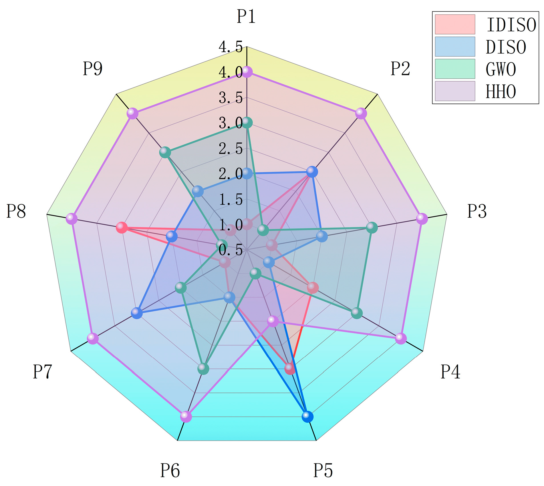
| Algorithm | P1 | P2 | P3 | P4 | P5 | P6 | P7 | P8 | P9 | Average | Final |
|---|---|---|---|---|---|---|---|---|---|---|---|
| IDISO | 1 | 2.5 | 1 | 2 | 3 | 1.5 | 1 | 3 | 1 | 1.7778 | 1 |
| DISO | 2 | 2.5 | 2 | 1 | 4 | 1.5 | 3 | 2 | 2 | 2.3333 | 3 |
| GWO | 3 | 1 | 3 | 3 | 1 | 3 | 2 | 1 | 3 | 2.2222 | 2 |
| HHO | 4 | 4 | 4 | 4 | 2 | 4 | 4 | 4 | 4 | 3.6667 | 4 |
| Learning Rate | Number of Trees | Depth of the Tree | The Proportion of Subsamples Sampled | Regular Term Coefficient | Val_R2 | Test_R2 | |
|---|---|---|---|---|---|---|---|
| upper and lower bounds | [0.01–1] | [100–1000] | [3–10] | [0.01–0.3] | [0.01–0.05] | ||
| IDISO_C | 2.9846157 × 10⁻¹ | 655 | 10 | 3.8879849 × 10⁻¹ | 3.3397663 × 10⁻² | 0.97 | 0.95 |
| DISO_C | 2.25181533 × 10⁻¹ | 549 | 9 | 1.92181424 × 10⁻¹ | 4.15709607 × 10⁻² | 0.96 | 0.92 |
| IDISO_H | 2.95662070 × 10⁻¹ | 407 | 3 | 2.53441246 × 10⁻¹ | 4.78747122 × 10⁻² | 0.97 | 0.96 |
| DISO_H | 4.68936589 × 10⁻¹ | 233 | 6 | 2.15128044 × 10⁻¹ | 2.02117095 × 10⁻² | 0.95 | 0.93 |
| IDISO_O | 7.053795 × 10⁻² | 659 | 6 | 5.638555 × 10⁻¹ | 3.864307 × 10⁻² | 0.97 | 0.96 |
| DISO_O | 4.65478169 × 10⁻¹ | 569 | 8 | 2.33724901 × 10⁻¹ | 1.24724460 × 10⁻² | 0.93 | 0.91 |
| IDISO_N | 8.1734951 × 10⁻² | 533 | 8 | 5.5392384 × 10⁻¹ | 3.5553879 × 10⁻² | 0.95 | 0.94 |
| DISO_N | 7.38914069 × 10⁻¹ | 997 | 8 | 2.26746118 × 10⁻¹ | 4.19970431 × 10⁻² | 0.90 | 0.89 |
Disclaimer/Publisher’s Note: The statements, opinions and data contained in all publications are solely those of the individual author(s) and contributor(s) and not of MDPI and/or the editor(s). MDPI and/or the editor(s) disclaim responsibility for any injury to people or property resulting from any ideas, methods, instructions or products referred to in the content. |
© 2024 by the authors. Licensee MDPI, Basel, Switzerland. This article is an open access article distributed under the terms and conditions of the Creative Commons Attribution (CC BY) license (https://creativecommons.org/licenses/by/4.0/).
Share and Cite
Shi, J.; Zhang, D.; Sui, Z.; Wu, J.; Zhang, Z.; Hu, W.; Huo, Z.; Wu, Y. Improved Dujiangyan Irrigation System Optimization (IDISO): A Novel Metaheuristic Algorithm for Hydrochar Characteristics. Processes 2024, 12, 1321. https://doi.org/10.3390/pr12071321
Shi J, Zhang D, Sui Z, Wu J, Zhang Z, Hu W, Huo Z, Wu Y. Improved Dujiangyan Irrigation System Optimization (IDISO): A Novel Metaheuristic Algorithm for Hydrochar Characteristics. Processes. 2024; 12(7):1321. https://doi.org/10.3390/pr12071321
Chicago/Turabian StyleShi, Jingyuan, Dapeng Zhang, Zifeng Sui, Jie Wu, Zifeng Zhang, Wenjie Hu, Zhanpeng Huo, and Yongfu Wu. 2024. "Improved Dujiangyan Irrigation System Optimization (IDISO): A Novel Metaheuristic Algorithm for Hydrochar Characteristics" Processes 12, no. 7: 1321. https://doi.org/10.3390/pr12071321
APA StyleShi, J., Zhang, D., Sui, Z., Wu, J., Zhang, Z., Hu, W., Huo, Z., & Wu, Y. (2024). Improved Dujiangyan Irrigation System Optimization (IDISO): A Novel Metaheuristic Algorithm for Hydrochar Characteristics. Processes, 12(7), 1321. https://doi.org/10.3390/pr12071321