Evaluation of Key Development Factors of a Buried Hill Reservoir in the Eastern South China Sea: Nonlinear Component Seepage Model Coupled with EDFM

Abstract

The HZ 26-B buried hill reservoir is located in the eastern part of the South China Sea. This reservoir is characterized by the development of natural fractures, a high density, and a complex geological structure, featuring an upper condensate gas layer and a lower volatile oil layer. These characteristics present significant challenges for oilfield exploration. To address these challenges, this study employed advanced embedded discrete fracture methods to conduct comprehensive numerical simulations of the fractured buried hill reservoirs. By meticulously characterizing the flow mechanisms within these reservoirs, the study not only reveals their unique characteristics but also establishes an embedded discrete fracture numerical model at the oilfield scale. Furthermore, a combination of single-factor sensitivity analysis and the Pearson correlation coefficient method was used to identify the primary controlling factors affecting the development of complex condensate reservoirs in ancient buried hills. The results indicate that the main factors influencing the production capacity are the matrix permeability, geomechanical effects, and natural fracture length. In contrast, the impact of the threshold pressure gradient and bottomhole flow pressure is relatively weak. This study’s findings provide a scientific basis for the efficient development of the HZ 26-B oilfield and offer valuable references and insights for the exploration and development of similar fractured buried hill reservoirs.

1. Introduction

Buried hills are reservoirs where hydrocarbons accumulate beneath unconformities, formed in traps created by ancient topographical uplifts. These reservoirs typically have favorable structural settings and conditions, making them important in oil and gas exploration. The exploration and development of buried hill reservoirs hold a significant position in the global petroleum industry, especially under complex geological conditions [1,2]. In recent years, with the maturity of oil and gas exploration technology and the increase in exploration efforts in China, bedrock buried hill oil and gas reservoirs have been discovered one after another. Their position in mature oil and gas exploration and development is increasingly prominent [3]. The primary pores of the bedrock buried hill reservoir are poorly developed, and fractures become its main storage and permeability space [4,5,6]. The existence and development degree of fractures play a crucial role in the migration and accumulation of fluids [7]. Natural fractures usually exist in network forms with complex geometries and connectivity [8]. These fractures can significantly enhance the permeability of the reservoir and the fluid flow capability. As the main flow channels, fractures have high permeability but limited storage capacity. Fluid flow within fractures follows Darcy’s law under low flow rate conditions, whereas non-Darcy flow effects need to be considered under high flow rate conditions. Therefore, how to accurately describe and simulate the flow behavior of fluids in fractures has become a key issue that urgently needs to be solved in the exploration and development of buried hill reservoirs. This is not only related to a deep understanding of the characteristics of buried hill reservoirs but also an important prerequisite for providing a scientific basis for the design of development plans for fractured reservoirs in buried hills [9,10,11]. There are currently some mature technological achievements in the construction of models for fractures, which can be mainly divided into three categories.

(1)

Equivalent continuum model (ECM)

In the equivalent medium model, the high conductivity of fractures is evenly distributed to a portion of the grid to achieve the equivalent treatment of fractures. This type of model is derived from the evolution of general single-pore medium models and was first studied for single-pore sandstone reservoirs. Barenblatt proposed, for the first time, the construction of fractured media to reflect the characteristics of seepage in order to reflect the differences between the primary intergranular pores of the reservoir matrix and the pores of the fracture system [12]. Warren and Root first introduced this dual medium model into petroleum engineering applications and provided a complete mathematical explanation and model building method [13]. The advantage of the equivalent continuous medium model lies in its ease of applying mature theories of porous media seepage. However, the assumption that fractures are evenly divided into matrix grids differs significantly from the actual reservoir situation. This also poses certain difficulties in determining the size parameters of the fractured medium unit and the equivalent fracture permeability [14].

(2)

Discrete fracture model (DFM)

The discrete fracture model was established to characterize the significant differences in the geometric shape and spatial distribution of fractures. By ignoring the width of the fractures, they are dimensionally reduced and embedded on the intersection surface of the matrix grid [15]. The discrete fracture model can accurately characterize fractures compared to the equivalent continuous medium model. The discrete fracture model can establish a realistic fracture seepage model through factors such as fracture geometry and spatial distribution. Kim et al. applied DFM to oil-water two-phase flow [16]. They believe that DFM has good adaptability when there are significant scale differences between the matrix and fractures. Helnemann et al. applied unstructured grids for the first time in numerical simulations, using finite volume discretization methods for the solution. Verma further provided some two-dimensional and three-dimensional mesh generation methods (PEBI) under specific boundary conditions and conducted numerical simulation calculations [17]. Denney et al. summarized the mesh partitioning methods for discrete fracture models [18]. They believe that the division of unstructured grids does not lead to a decrease in computational accuracy but instead increases the difficulty of running numerical models, resulting in a decrease in computational efficiency.

(3)

Embedded Discrete Fracture Model (EDFM)

An embedded discrete fracture model (EDFM) is proposed using a rectangular grid discrete matrix, with the fracture grid determined by its intersection with the matrix grid [19,20]. Lee achieved coupling between the matrix and fracture systems by converting fracture conductivity into a source sink term in the matrix grid continuity equation [21]. Moinfar et al. extended the EDFM model to three-dimensional space, analyzed the effects of natural and hydraulic fractures on seepage pressure and saturation fields, and conducted a productivity analysis of horizontal wells [22]. The work of these two scholars is considered to have laid the foundation for the application of EDFM models. EDFM has been promoted in petroleum engineering [23]. Rao et al. investigated the errors generated by the assumption of linear pressure distribution, targeting the matrix elements at the boundaries of embedded discrete fracture models [24]. Furthermore, a multi-layer grid refinement method was proposed, which improved the accuracy of the model, with low impact on computational efficiency. The embedded discrete fracture model preserves the structured matrix grid and embeds fractures into the matrix grid to form a fracture matrix seepage system. EDFM effectively retains the advantages of DFM in explicitly representing fractures while also providing a more general representation of fracture distribution. This method not only considers the precise description of fractures but also reduces the difficulty and computational requirements of building models [25,26,27].

In summary, compared to ECM, EDFM has significant advantages in handling complex fracture networks and improving numerical simulation accuracy. ECM typically assumes that the fracture network is uniform and regular, making it difficult to address complex fracture geometries. In contrast, EDFM can flexibly manage intricate fracture networks, including randomly distributed fractures, heterogeneous fractures, and intersecting fractures. Therefore, in this study, EDFM will be used to simulate fractures in buried hill reservoirs.

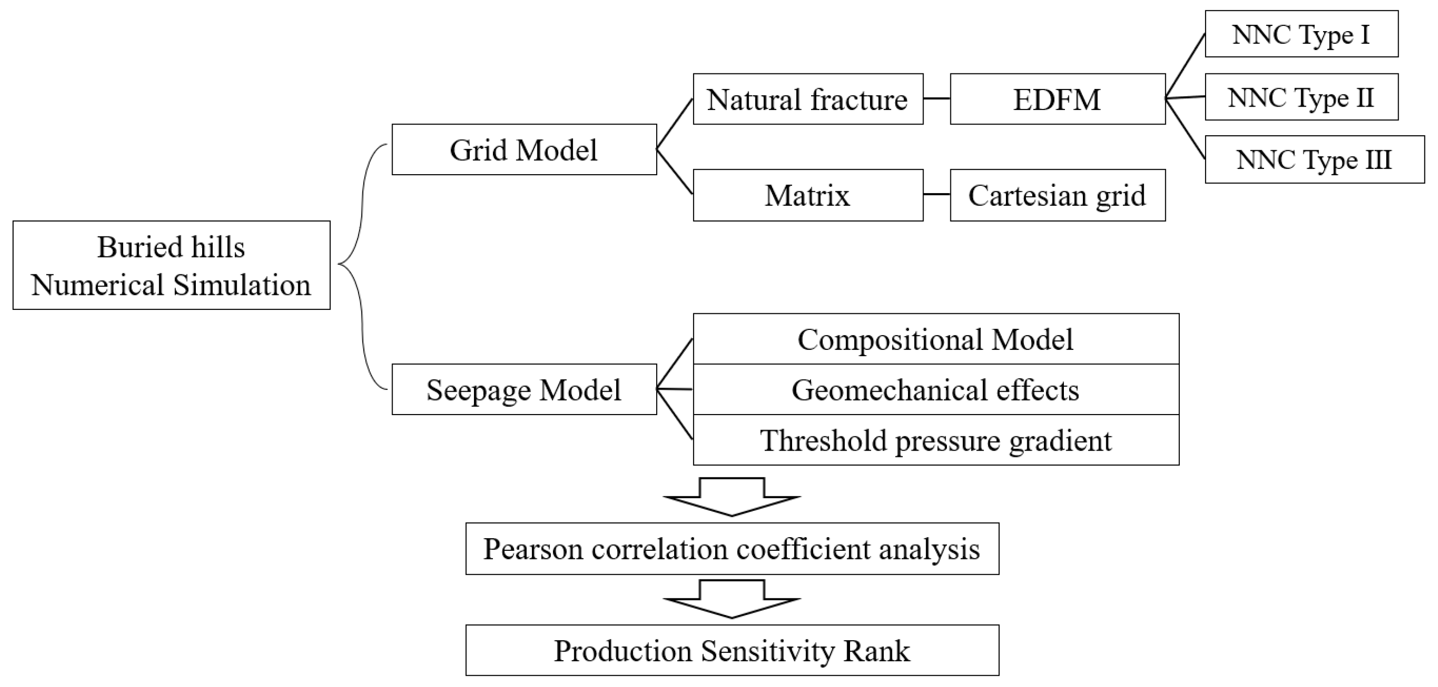
2. Materials and Methods

In this study, a reservoir-scale numerical model was established using the HZ 26-B buried hill reservoir as an example. The model is based on the EDFM technique, which explicitly characterizes natural fractures throughout the region and considers the threshold pressure gradient and geomechanical effects of the tight reservoir. Finally, sensitivity analysis was conducted, and the primary controlling factors were ranked using the Pearson correlation coefficient method. The framework flowchart of the entire manuscript is shown in Figure 1.

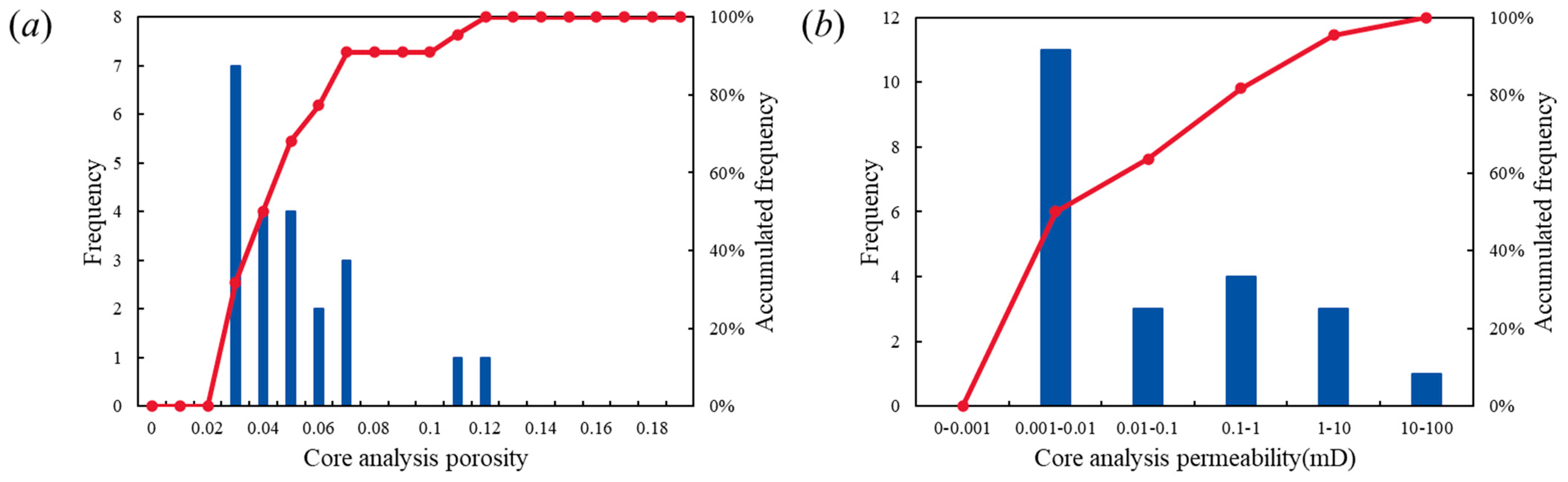
2.1. Geological Setting

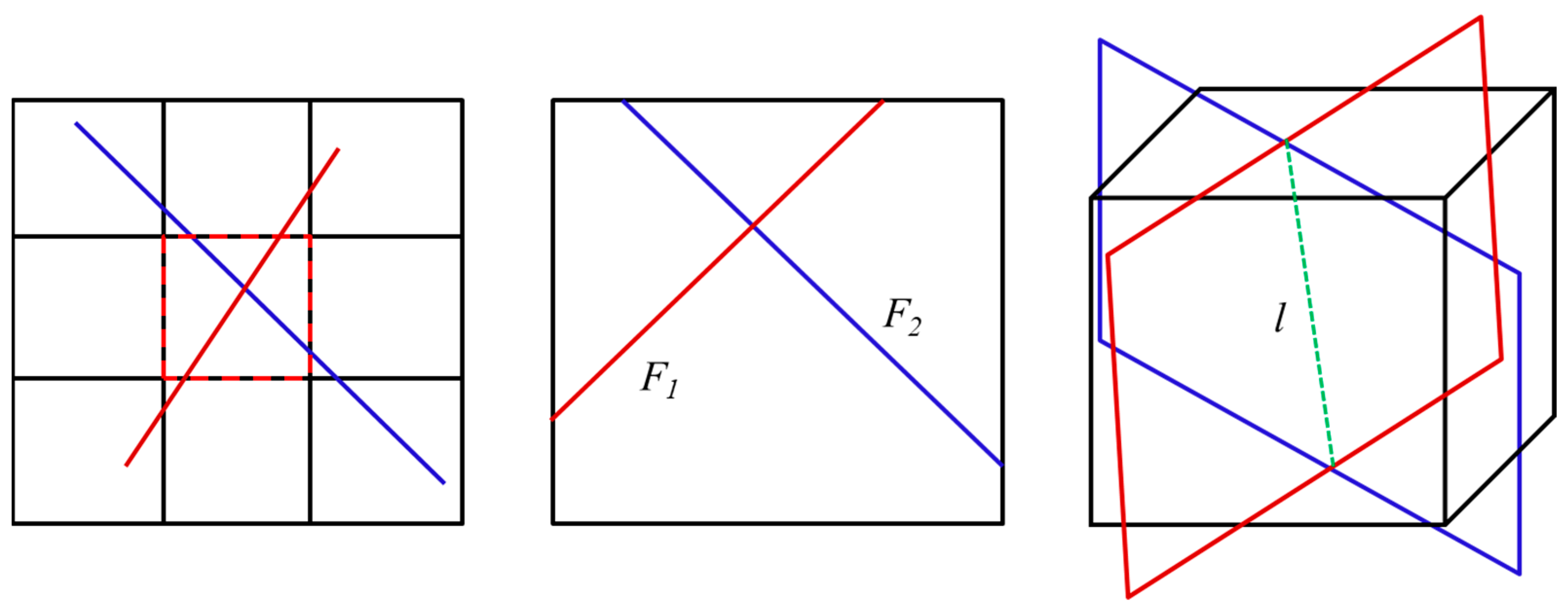
The HZ 26-B structure is located in the southern composite fault zone of Huizhou Sag, the Pearl River Mouth Basin. It is a composite trap composed of Mesozoic block-shaped buried hills and their overlying Paleogene Wenchang Enping Formation layered sandstones and gravel rocks. The main target layer is the Enping Formation of the Paleogene, which is a fault nose structure, while the Wenchang Formation and the ancient buried hill are complex fault anticline structures with the advantages of a complete trap morphology, high overlap, and large area. The analysis of core, wall, and imaging logging data shows that the macroscopic natural fractures of the Mesozoic buried hill in the HZ 26-B oilfield are well developed. The cutting relationship and filling situation of natural fractures are complex, and a multi-stage fracture system is developed. The weathering fracture zone has formed a network of fracture systems. Due to the superimposed physical and chemical weathering and leaching effects, weathering fracture zones and other areas are severely fractured due to stress. The imaging logging interpretation of fractures mainly consists of unfilled and partially filled open fractures. As shown in Figure 2, the statistical analysis shows that the fracture direction is mainly northwest–southeast and northeast–southwest, and the fracture dip angle is mainly 30–70 degree medium-and-high-angle oblique joints, followed by 10–30 degree low-angle oblique joints, with the least horizontal joints less than 10 degrees and the vertical joints greater than 80 degrees. The density of single-well fractures ranges from 4.6 to 6.2 per meter.

The reservoir space of the ancient buried hill exhibits obvious dual-pore characteristics, and its reservoir heterogeneity is significant. Figure 3 displays the core analysis results, indicating that the porosity of the reservoir falls between 2.0% and 11.4%, with an average of 4.6%. Meanwhile, the permeability of the region ranges from 0.001 mD to 31.6 mD, with an average of 2.04 mD. Further logging interpretation results show that the porosity fluctuates between 2.0% and 17.1%, with an average of 5.3% and a median of 4.8%. The permeability exhibits greater variability, ranging from 0.019 mD to 64.3 mD, with an average value of 3.3 mD. According to the classification of non clastic rock reservoirs, ancient buried hills are mainly composed of low-to-medium-porosity and ultra-low-permeability reservoirs. It reveals the complexity and heterogeneity of ancient buried hill reservoirs.

The research area is currently in the trial production stage and has not undergone large-scale development. The aim of this study is to establish a complex geological model through numerical simulation methods. Based on the simulation results, a sensitivity analysis will be conducted to identify the main factors affecting production capacity. This will provide clear guidance for subsequent large-scale development.

2.2. EDFM Model

In the embedded discrete fracture model, hydraulic fractures and natural bedding planes are inserted into the matrix grid and are split into several sections, each of which is a fracture step. The exchange of matter between the matrix and the fractures, or between different fractures, is carried out through non-adjacent connections (NNCs), and the amount of matter exchanged can be expressed as the product of the conductance rates between the units and the pressure differences:

$$q=T\left(p_1-p_2\right)$$

There are three types of NNC material exchanges in the embedded discrete fracture model, and the conductive rates differ between various modes of exchange.

2.2.1. NNC Type I: Connection between a Fracture Segment and the Matrix Cell

Fractures within individual matrix grids are divided into separate segments. As depicted in Figure 4, these fracture segments have a polygonal interface with the matrix grid, through which the flow of matter between the fracture system and the matrix system is exchanged. Therefore, the computation of the physical exchange between the matrix and the fractures within a single grid is identical to the computation of the physical exchange between the matrix and the fracture faces.

The conductivity rate of a single fracture through the matrix grid is

$$T_{mF}={\displaystyle \frac{A_F}{\overline{d}}}{k}_{mF}$$

where A_F represents the area of the interface between the fracture and the matrix, m; k_m is the harmonic mean of the permeabilities of the matrix and the fractures; and $\overline{d}$ is the average distance from the matrix to the interface.

The calculation method for the harmonic average of matrix and fracture permeability is as follows:

$$k_{mF}={\displaystyle \frac{1}{k_m}}+{\displaystyle \frac{1}{k_F}}$$

Among them, k_m is the matrix permeability, and k_F is the permeability of the fracture.

$\overline{d}$ refers to the distance between a representative point on the matrix and a representative point on the fracture surface, calculated by the formula shown below.

$$\overline{d}={\displaystyle \frac{1}{V}}{\displaystyle \underset{V}{\int }{x}_{n}dV}$$

Among them, V is the volume of the matrix grid, and x_n is the distance from each differential pressure point on the matrix to the fracture.

2.2.2. NNC Type II: The Interconnection between Two Different Fractures within the Same Grid

Two intersecting fractures within the same porous medium will create a line of intersection. The exchange of materials between these two fractures happens through this line of intersection. As shown in Figure 5, there is a line of intersection between the two fragments of the fractured zone. Through this line of intersection, there is a material exchange between the two sides of the fracture.

$$T_1={\displaystyle \frac{w_{F1}l}{d_{F1}}}{k}_{F1},T_2={\displaystyle \frac{w_{F2}l}{d_{F2}}}{k}_{F2}$$

Among them, w_F1 and w_F2 are the openings of two fractures, respectively; l is the length of the intersection line between fracture fragments; k_F1 and k_F2 are the permeabilities of two fractures, respectively; and d_F1 and d_F2 are the average distances from two fractures to the intersection line, respectively.

2.2.3. NNC Type III: Connection of the Same Fracture within Different Grids

When a fracture passes through different matrix grids simultaneously, there is a flow exchange between the fracture and both matrix grids. As shown in Figure 6, there will be an intersection line between the penetrating fracture pieces and the two matrix grids. The fracture exchanges material with two matrix grids through this intersection line. For NNC type III, material exchange occurs between the fracture and the matrix grid through the 0 intersection line, and the conductivity can be directly expressed as the conductivity between the fracture and the intersection line:

$$T_F={\displaystyle \frac{w_F{l}_F}{d_F}}{k}_F$$

The EDFM model mainly exchanges materials through the above three NNCs. When multiple fractures intersect with multiple matrix grids, it is extremely important to distinguish the NNC types. Based on the above embedded discrete fracture calculation method combined with basic seepage mechanics theory, the general equation for fluid seepage in NNC fractures can be written:

$$q_{nnc}={\displaystyle \sum _{m=1}^{n_{nnc}}{A}_m^{nnc}\cdot \frac{k_m^{nnc}{k}_{ri}}{{\mu }_i}{\rho }_i{x}_i\left[\frac{\left(p-\gamma D\right)-{\left(p-\gamma D\right)}_m^{nnc}}{d_m^{nnc}}\right]}$$

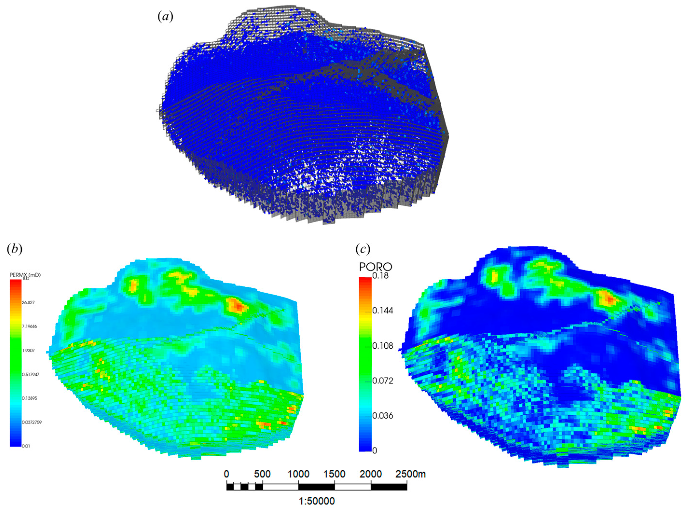
2.3. Reservoir Numerical Simulation Model

Based on the component model of fractured oil and gas reservoirs, the establishment of seepage equations is the key to describing the migration behavior of oil and gas in the reservoir. This equation comprehensively considers the two-phase flow characteristics of oil and gas in fractures and matrices, as well as the interactions between oil and gas components. By introducing appropriate flow coefficients and equilibrium relationships, the equation can accurately describe the fluid flow process in the reservoir. According to the material balance equation, the cumulative change in fluid is equal to the sum of the flow term and the source sink term. The permeation equation for component i in the oil phase of the matrix can be written:

$$\nabla \left[{\displaystyle \sum _{i=1}^n{x}_i^m}\left({\displaystyle \frac{{\rho }_o{k}^m{k}_{ro}^m}{{\mu }_o}}\nabla p_o^m\right)\right]-{\displaystyle \sum _{i=1}^n{x}_i^m}{q}_o^{mf}={\displaystyle \frac{\partial }{\partial t}}\left[{\varphi }^m{S}_o^m{x}_i{\rho }_o\right]$$

Among them, o represents the oil phase, i represents component i, x_i represents the molar fraction of component i in the oil phase, ρ_o is the oil density, μ_o is the oil viscosity, $k_{ro}^m$ is the relative permeability of the oil phase in the matrix, and k^m is the matrix permeability, which has taken into account the stress sensitive effect and is corrected by the following formula:

$$k^m=k_0^m{e}^{-\beta \left(p_0-p\right)}$$

$q_o^{mf}$ is the flow exchange of the oil phase in the matrix and fractures, which can be expressed as

$$q_o^{mf}=q_{nnc}={\displaystyle \sum _{m=1}^{n_{nnc}}{A}_m^{nnc}\cdot \frac{k_m^{nnc}{k}_{ro}}{{\mu }_o}{\rho }_o{x}_o\left[\frac{\left(p_o-{\gamma }_{o}D\right)-{\left(p_o-{\gamma }_{o}D\right)}_m^{NNC}}{d_m^{nnc}}\right]}$$

Similarly, the gas phase permeation equation for component i in the matrix can be expressed as

$$\nabla \left[{\displaystyle \sum _{i=1}^n{y}_i^m}\left({\displaystyle \frac{{\rho }_o{k}^m{k}_{rg}^m}{{\mu }_g}}\nabla p_g^m\right)\right]-{\displaystyle \sum _{i=1}^n{y}_i^m}{q}_g^{mf}={\displaystyle \frac{\partial }{\partial t}}\left[{\varphi }^m{S}_g^m{y}_i{\rho }_g+m_g\right]$$

$$q_g^{mf}=q_{nnc}={\displaystyle \sum _{m=1}^{n_{nnc}}{A}_m^{nnc}\cdot \frac{k_m^{nnc}{k}_{rg}}{{\mu }_g}{\rho }_g{y}_g\left[\frac{\left(p_g-{\gamma }_{g}D\right)-{\left(p_g-\gamma {}_{g}D\right)}_m^{NNC}}{d_m^{nnc}}\right]}$$

Among them, _g represents the gas phase, _i represents component i, y_i represents the molar fraction of component i in the gas phase; ρ_g is the gas density; μ_g is the gas viscosity; and $k_{rg}^m$ is the relative permeability of the gas in the matrix.

The water phase, as a separate component, does not consider material exchange with oil and gas. The permeation equation of water in the matrix is

$$\nabla \left[\left({\displaystyle \frac{{\rho }_o{k}^m{k}_{rw}^m}{{\mu }_w}}\nabla p_w^m\right)\right]-q_w^{mf}={\displaystyle \frac{\partial }{\partial t}}\left[{\varphi }^m{S}_w^m{\rho }_w\right]$$

$$q_w^{mf}=q_{nnc}={\displaystyle \sum _{m=1}^{n_{nnc}}{A}_m^{nnc}\cdot \frac{k_m^{nnc}{k}_{rw}}{{\mu }_w}{\rho }_w{y}_w\left[\frac{\left(p_w-{\gamma }_{w}D\right)-{\left(p_w-{\gamma }_{w}D\right)}_m^{NNC}}{d_m^{nnc}}\right]}$$

Among them, w represents the Water phase; ρ_w is the water density; μ_w is the water viscosity; and $k_{rw}^m$ is the relative permeability of water in the matrix.

Similar to the seepage equation in the matrix, the seepage equations for oil and gas phases in fractures are

$$\nabla \left[{\displaystyle \sum _{i=1}^n{x}_i^m}\left({\displaystyle \frac{{\rho }_o{k}^f{k}_{ro}^f}{{\mu }_o}}\nabla p_o^f\right)\right]+{\displaystyle \sum _{i=1}^n{x}_i^f}{q}_o^{mf}-q_o^{well}={\displaystyle \frac{\partial }{\partial t}}\left[{\varphi }^f{S}_o^f{x}_i{\rho }_o\right]$$

$$\nabla \left[{\displaystyle \sum _{i=1}^n{y}_i^f}\left({\displaystyle \frac{{\rho }_o{k}^f{k}_{rg}^f}{{\mu }_g}}\nabla p_g^f\right)\right]+{\displaystyle \sum _{i=1}^n{y}_i^f}{q}_g^{mf}-q_g^{well}={\displaystyle \frac{\partial }{\partial t}}\left[{\varphi }^f{S}_g^f{y}_i{\rho }_g\right]$$

Among them, $q_o^{well}$ and $q_g^{well}$ is the source sink term for the exchange of materials between the fracture and the wellbore.

For low-permeability reservoirs, the radius of the seepage channel is generally at the micro–nano scale, and the boundary layer plays a significant role. The fluid undergoes low-speed non-Darcy seepage in the seepage channel, and the influence of the threshold pressure gradient on the flow cannot be ignored. The following equation is the seepage motion equation considering the threshold pressure gradient:

$$v=\left\{\begin{array}{c}0,\left|\nabla \psi \right|\le G\\ -{\displaystyle \frac{K{K}_r}{\mu }}\left(1-{\displaystyle \frac{G}{\left|\nabla \psi \right|}}\right)\nabla \psi ,\left|\nabla \psi \right|>G\end{array}\right.$$

Among them, $\nabla \psi$ represents the production pressure difference, K represents permeability, K_r is the relative permeability, μ is the fluid viscosity, and G is the threshold pressure gradient.

As shown in Figure 7, based on a numerical simulator, we established a filed-scale numerical model with a grid count of 152 × 92 × 400 and a grid step size of 50 × 50 × 2.5. Figure 7a shows the 72,593 natural fractures established using EDFM technology. Figure 7b displays the distribution of matrix permeability in the model, while Figure 7c illustrates the distribution of matrix porosity. For the HZ 26-B buried hill reservoir, the structure, properties, and discrete fracture model are derived from geological modeling. The relevant parameters are shown in

Table 1. Numerical simulation model attribute parameters.

Content		Parameter	Unit
Grid number		152 × 92 × 400
Grid size		50 × 50 × 2.5	m
Matrix permeability	Maximum permeability	95.8	mD
	Minimum permeability	0.06
	Average permeability	1.2
Matrix porosity	Minimum porosity	0.5	%
	Maximum porosity	17.9
	Average porosity	3.7
Natural fractures in Weathering Zones	Fracture trend	158	°
	Fracture dip angle	52	°
	Fracture density	4.4	piece/m
	Fracture aperture	55	μm
Natural fractures in the inner zone	Fracture trend	138	°
	Fracture dip angle	57	°
	Fracture density	3.7	piece/m
	Fracture aperture	49	μm

.

To avoid changes in reserves caused by the shrinkage of matrix porosity, and to prevent fractures from being used as storage spaces, changes in porosity with stress are not considered. The stress sensitivity curve is shown in Figure 8. This curve indicates that as the pressure decreases, the fracture permeability also decreases, with the degree of change being the product of the initial permeability and the stress sensitivity multiplier.

According to the analysis results of the threshold pressure gradient experiment, as shown in Figure 9, considering only the presence of a threshold pressure gradient in single-phase oil, under the condition of an average permeability of 1.2 mD, the threshold pressure gradient is set to 0.02 MPa/m.

The fluid type in the weathering zone of HZ 26-B is condensate gas, and the numerical simulation process considers the use of component models for simulation. The fluid components are primarily composed of methane, ethane, and propane, with small amounts of carbon dioxide and nitrogen. The saturation pressure of the condensate gas is 37.86 MPa, which is very close to the formation pressure of 38.8 MPa, classifying it as a near-critical fluid. The properties of each component of the fluid are shown in

Table 2. Parameters of each pseudo-component of the fluid.

Pseudo- Component	Critical Pressure	Critical Temperature	Critical Volume	Molar Mass	Mole Fraction
	bar	K	m3/kg·mol
N2-C1	45.97	190.45	0.10	16.07	68.01%
CO2-C2	48.87	305.23	0.15	30.12	8.31%
C3	42.46	369.80	0.20	44.10	15.46%
C4-C6	32.76	471.30	0.32	73.95	3.09%
C7-C10	28.04	631.61	0.72	141.64	4.97%
C11+	16.07	975.02	2.47	530.82	0.15%

, and the fluid phase diagram is shown in Figure 10.

We consider using different permeability curves for the matrix and fracture systems, where the matrix permeability curve is obtained from experiments, as shown in Figure 11a, while the empirical curve is used for the relative permeability of the natural fracture system, as shown in Figure 11b.

Based on the above parameter settings, we performed a historical match on the research block. Forty-five continuous and effective data points were selected, and the fixed gas production rate was used to fit the bottomhole flow pressure. As shown in Figure 12, the curve fitting accuracy was 92%.

3. Discussion

In this study, an in-depth analysis was conducted on the sensitivity of four key factors: threshold pressure, stress sensitivity effect, natural fractures density, and fractures length based on the established numerical model of an ancient buried hill reservoir.

(1)

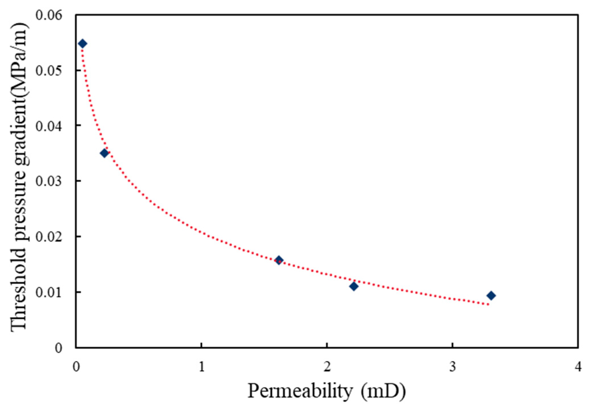
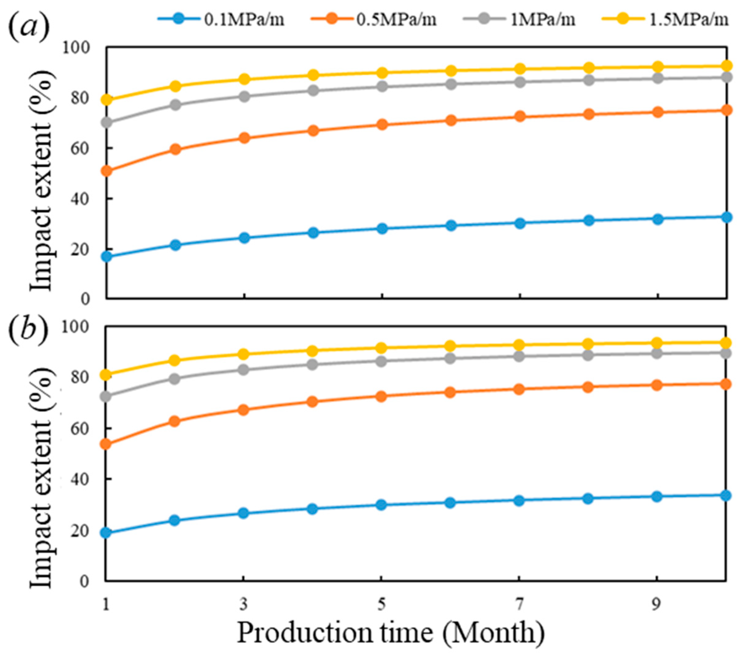
Sensitivity analysis of threshold pressure

In numerical simulation research, we carefully selected the range of the threshold pressure gradient, extending from 0.1 MPa/m to 1.5 MPa/m. Research has found that as the threshold pressure gradient of the reservoir increases, the initial production of oil and gas shows a downward trend, and its depletion rate accelerates, resulting in a corresponding decrease in cumulative production. When the threshold pressure gradient is set to 0.1 MPa/m, its impact on oil and gas production is relatively mild, with an average impact degree of about 27.5%. However, once the threshold pressure gradient exceeds 0.5 MPa/m, the degree of influence sharply increases, exceeding 50%, as shown in Figure 13.

The introduction of a threshold pressure gradient has a significant impact on pressure propagation. Under the condition of a threshold pressure gradient of only 0.1 MPa/m, after one year of oil and gas development, the pressure ripple radius can reach about 1600 m, showing a relatively wide range of influence. When the threshold pressure gradient increases to 1.5 MPa/m, the radius of this wave significantly decreases to about 400 m, reflecting a more rapid pressure attenuation. This trend of change is clearly shown in Figure 14, which intuitively reveals the important influence of the threshold pressure gradient on the range of pressure propagation.

(2)

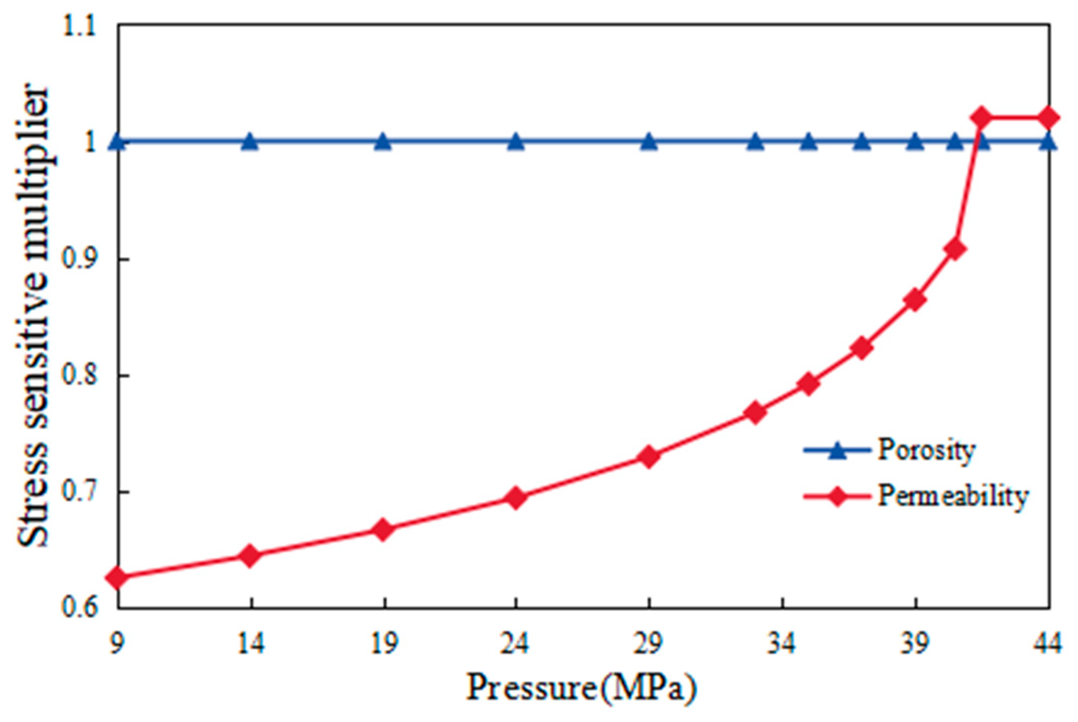
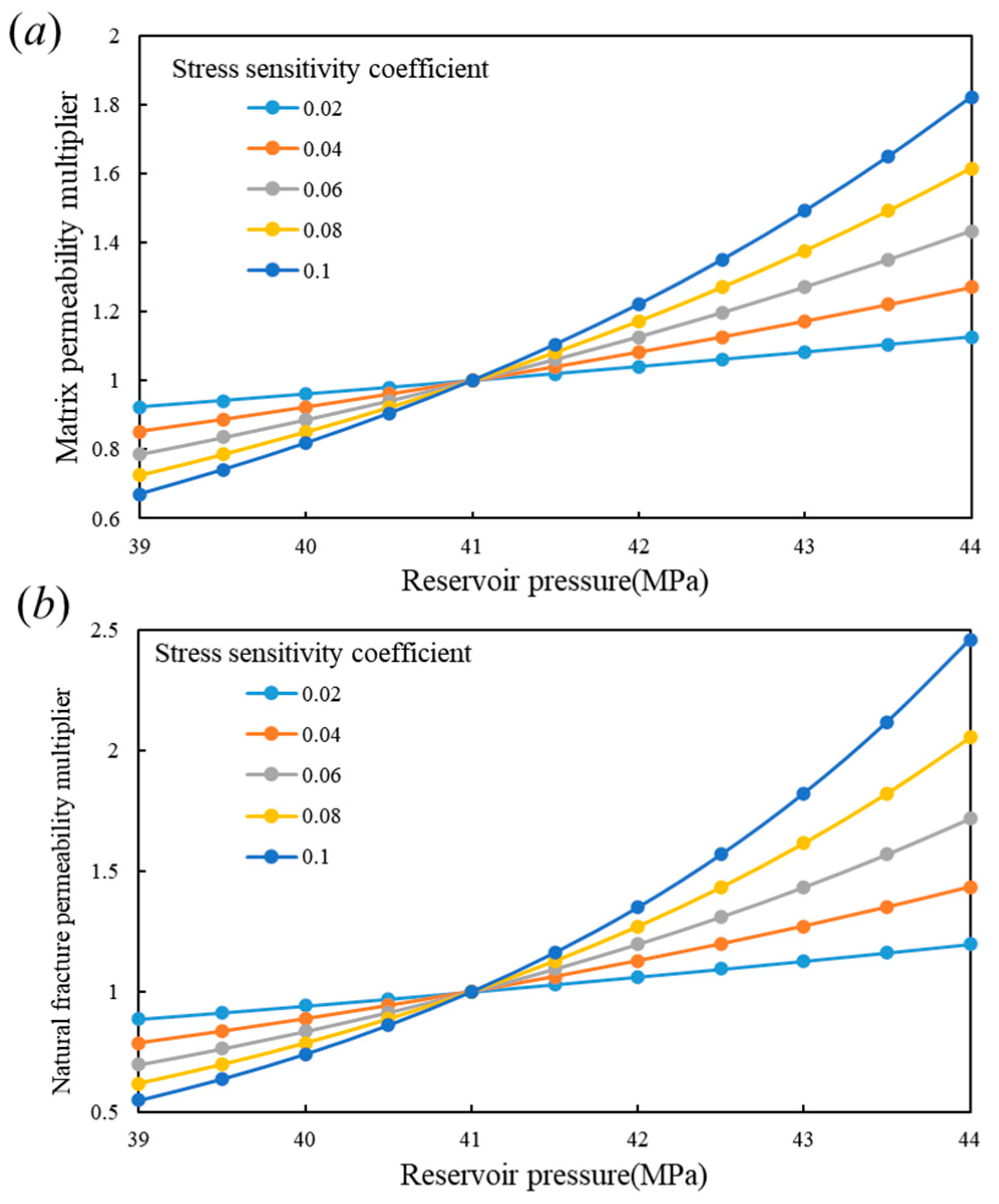
Sensitivity analysis of geomechanical effects

Based on the previous stress sensitivity research data, we have selected a range of stress sensitivity coefficients between 0.01 and 0.1 to conduct this stress sensitivity analysis. In the analysis process, in order to avoid potential reserve changes caused by the shrinkage of matrix porosity due to stress, and considering that fractures do not directly serve as storage spaces, we deliberately excluded the factor of porosity changing with stress. The research results reveal that under the same stress conditions, the degree of influence of various factors on reservoir performance is ranked in the following order: natural fracture porosity has the smallest impact, followed by matrix porosity, followed by matrix permeability, and natural fracture permeability has the greatest impact. This ranking remains consistent under different stress sensitivity coefficient conditions, and the related trend can be intuitively observed in Figure 15.

With the enhancement of the stress sensitivity effect, the initial production of condensate gas wells shows a downward trend, and its cumulative production also correspondingly decreases. If the stress sensitivity coefficient is high within the same production cycle, it indicates that the impact of stress sensitivity on the yield is more significant. However, as the development time continues, the impact of stress sensitivity will gradually weaken. Specifically, when the stress sensitivity coefficient is 0.02, its average impact on the yield is about 28.68%. When the stress sensitivity coefficient is increased to 0.1, the degree of influence significantly increases, reaching 97.78%. These changing trends are clearly reflected in the gas production characteristic curve (Figure 16) under different stress sensitivity conditions.

As shown in Figure 17, the impact trend of stress sensitivity on condensate oil is similar to that of condensate gas, but there are differences in specific values. In the case of a stress sensitivity coefficient of 0.02, the impact of stress on condensate oil production is about 28.56%, which is equivalent to the impact on condensate gas production. However, when the stress sensitivity coefficient exceeds 0.02, the impact of stress sensitivity on condensate oil is significantly lower than that on condensate gas. Taking a stress sensitivity coefficient of 0.1 as an example, its impact on condensate oil production differs the most from its impact on condensate gas production, reaching 12.24%. These differences are visually displayed in Figure 18, showing the oil production characteristic curves under different stress sensitivity conditions.

(3)

Sensitivity analysis of natural fracture density

By changing the number of embedded fractures while keeping the other conditions constant, we can delve deeper into the impact of fracture density on complex fractured oil and gas reservoirs. In the study, we considered fracture density conditions ranging from 1000 to 5000 to explore the impact of changes in fracture density on reservoir permeability characteristics.

Figure 19 shows that as the fracture density decreases, the pressure propagation speed of the fluid slows down and the propagation range becomes narrower. In addition, we also found that compared to the oil layer, the pressure depletion rate of the gas layer is faster, and the pressure wave shows a V-shaped propagation characteristic. This may be due to the poor permeability of the gas layer, making it easier for pressure to decay during propagation. In addition, fracture density also has a certain degree of influence on the degree of fracture development. In areas with high fracture development, due to the good connectivity of fractures, the oil and gas flow is smoother, resulting in relatively low saturation in the area. This effect is less pronounced in areas with lower levels of fracture development.

(4)

Sensitivity analysis of natural fracture length

As the length of the fracture increases, the initial production of oil and gas shows a significant growth trend, while the rate of depletion also accelerates significantly, ultimately leading to a significant increase in cumulative production. After a period of production, for different fracture lengths, the daily production showed a clear convergence trend, and the difference in daily production between different fracture lengths gradually narrowed. This phenomenon is visually shown in Figure 20.

This trend reflects the significant impact of fracture length on the development efficiency of oil and gas reservoirs. A longer fracture length helps to improve the flow of oil and gas, thereby increasing initial production. However, as the fault expands, the flow path of oil and gas may also become more complex, leading to an accelerated rate of depletion. However, in the long run, larger fracture lengths may still lead to higher cumulative production. In actual production, this means that for reservoirs with shorter fracture lengths, specific development measures may need to be taken to increase initial production and extend production life. For reservoirs with longer fracture lengths, although the initial production is higher, attention may need to be paid to optimizing production strategies to slow down the rate of depletion and achieve higher long-term cumulative production.

(5)

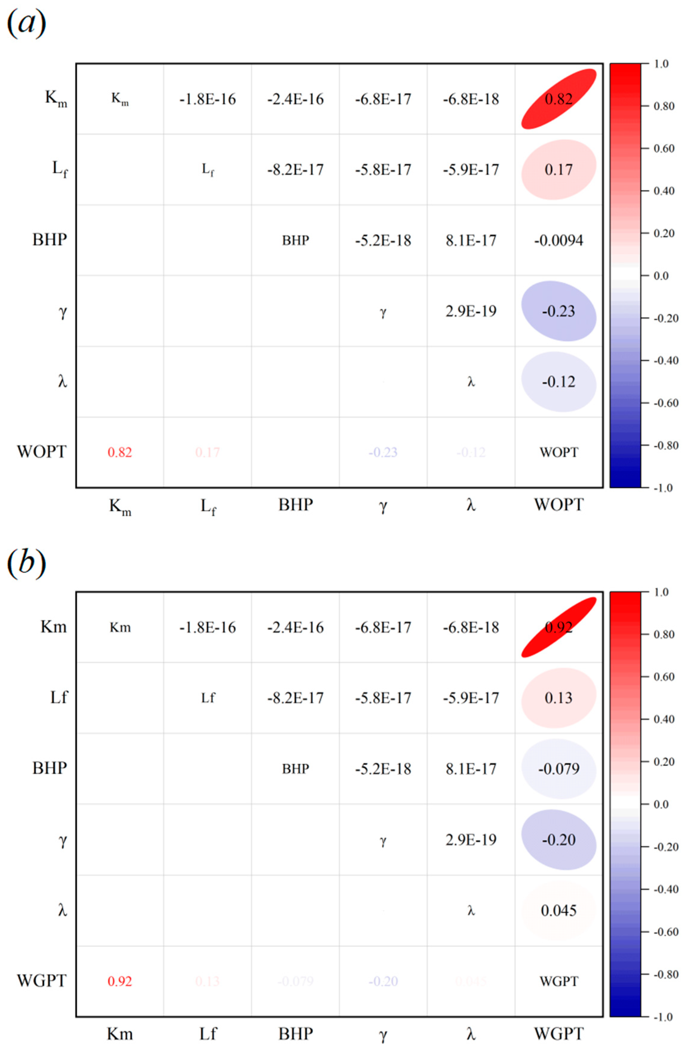
Pearson Correlation Coefficient

The Pearson correlation coefficient is a statistical tool used to measure the strength and direction of the linear relationship between two variables. Due to its simplicity, ease of use, and dimensionless properties, the Pearson correlation coefficient is frequently applied in various scientific and engineering fields for multi-factor evaluation. The Pearson correlation coefficient analysis method can clarify the relationship between production parameters and influencing factors. By identifying parameters highly correlated with the output, more effective production plans can be developed.

$$r={\displaystyle \frac{{\displaystyle \sum \left(x_i-\overline{x}\right)\left(y_i-\overline{y}\right)}}{\sqrt{{\displaystyle \sum {\left(x_i-\overline{x}\right)}^2{\displaystyle \sum {\left(y_i-\overline{y}\right)}^2}}}}}$$

where r represents the Pearson correlation coefficient, x_i and y_i represent observations of two variables, and $\overline{x}$ and $\overline{y}$ represent the average value of two variables.

Orthogonal experiments can greatly reduce the number of comprehensive experiments while covering as many combinations of parameters as possible and making different parameter combinations neat and evenly distributed. Therefore, orthogonal experimental design is used to establish a data sample set for production analysis.

According to the principle of orthogonal experimental design, the orthogonal experimental table adopts L₂₅(5⁵), indicating the existence of five factors and five levels in the table. Based on

Table 3. Orthogonal experiments and results.

Case	Km	lf	BHP	γ	λ	WGPT	WOPT
	md	m	MPa	/	MPa/m	106 m3	104 m3
1	0.01	50	15	0.02	0.1	1.04	0.55
2	0.01	100	20	0.04	0.5	0.55	0.38
3	0.01	150	25	0.06	1	0.39	0.31
4	0.01	200	30	0.08	1.5	0.31	0.24
5	0.01	250	35	0.1	2	0.22	0.14
6	0.1	50	20	0.06	1.5	0.92	2.13
7	0.1	100	25	0.08	2	0.8	1.79
8	0.1	150	30	0.1	0.1	1.25	1.49
9	0.1	200	35	0.02	0.5	1.97	1.39
10	0.1	250	15	0.04	1	1.77	2.83
11	1	50	25	0.1	0.5	4.25	12.68
12	1	100	30	0.02	1	10.32	24.21
13	1	150	35	0.04	1.5	3.6	10.51
14	1	200	15	0.06	2	5.69	17.94
15	1	250	20	0.08	0.1	5.39	14.54
16	5	50	30	0.04	2	22.83	71.07
17	5	100	35	0.06	0.1	33.17	55.26
18	5	150	15	0.08	0.5	21.34	67.38
19	5	200	20	0.1	1	17.96	58.28
20	5	250	25	0.02	1.5	41.74	114.39
21	10	50	35	0.08	1	22.3	70.92
22	10	100	15	0.1	1.5	33.23	109.12
23	10	150	20	0.02	2	63.47	180.52
24	10	200	25	0.04	0.1	112.13	174.96
25	10	250	30	0.06	0.5	48.62	123.78

K_m represents matrix permeability, l_f represents natural fracture length, BHP represents bottomhole flow pressure, γ represents stress sensitivity coefficient, λ represents threshold pressure gradient, WGPT represents well gas total production, and WOPT represents well oil total production.

, 25 sets of cases were simulated to obtain the cumulative gas and oil production for each set of cases, and the cumulative gas and oil production was used as response data.

Based on the above orthogonal experimental simulation results, the main controlling factors of production were analyzed according to the principle and steps of Pearson correlation coefficient analysis. The correlation degree between each factor and production is shown in Figure 21.

As shown in Figure 21, the red area represents the positive correlation coefficient, which is close to 1, indicating a strong positive correlation between the two variables, that is, the growth of one variable is accompanied by the synchronous growth of the other variable. The blue area represents the negative correlation coefficient, which is close to −1, indicating a clear negative correlation between two variables, that is, an increase in one variable will lead to a decrease in the other variable. The correlation coefficient of those white areas is close to 0, indicating a lack of a significant linear correlation between these two variables, and their changing trends may be independent of each other or influenced by other unconsidered factors.

As shown in Figure 21a, there is a strong orthogonal relationship between matrix permeability and cumulative oil production, which is shown in a deep red oval shape with a correlation coefficient of 0.82. The crack length shows a weak positive correlation with cumulative oil production, as shown in a light red oval shape in the graph, with a correlation coefficient of 0.17. The stress sensitivity coefficient and start-up pressure gradient show weak negative correlations with cumulative oil production, respectively. They are shown in a light blue oval shape in the graph, with correlation coefficients of −0.23 and −0.12. The correlation between bottomhole flow pressure and cumulative oil production is weak, approaching white in the matrix. As shown in Figure 21b, the above factors have a similar impact trend on cumulative gas production compared to cumulative oil production. However, for the starting pressure gradient, the impact on the oil phase is more significant.

In summary, for the HZ 26-B buried hill reservoir, the main factors affecting productivity are matrix permeability, geomechanical effects, and natural fracture length. The impact of the threshold pressure gradient and bottomhole flow pressure is relatively weak.

4. Conclusions

(1)

This study adopts embedded discrete fracture technology and combines geomechanical effects to deeply explore the stress sensitivity of the matrix and fractures, as well as the influence of the fluid initiation pressure gradient on fracture development in tight reservoirs. Based on these theoretical foundations, we have successfully constructed a highly accurate three-dimensional numerical model at the reservoir scale, which specifically simulates the fracture development characteristics of complex reservoirs in the HZ 26-B ancient buried hills.

(2)

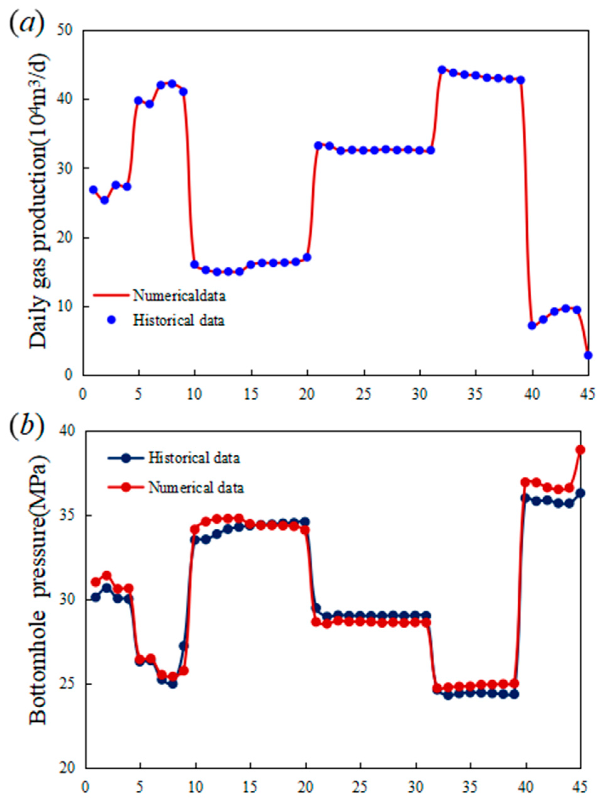
In the process of model construction, we made full use of on-site logging data and made precise corrections to the model, ensuring that the model output is highly consistent with the actual observation data. Through in-depth analysis of the model, we have revealed the impact mechanism of key factors such as the threshold pressure gradient, stress sensitivity coefficient, natural fracture density, and fracture length on reservoir productivity.

(3)

For the HZ 26-B buried hill reservoir, the main factors affecting productivity are the matrix permeability, geomechanical effects, and natural fracture length. The impact of the threshold pressure gradient and bottomhole flow pressure is relatively weak.

(4)

The research results indicate that these factors interact and together determine the development potential and production performance of oil and gas reservoirs. Especially, we found that the threshold pressure gradient has a significant impact on the initial production and pressure attenuation rate of oil and gas reservoirs, while the stress sensitivity coefficient is directly related to the degree of crack opening and expansion. In addition, the density and development characteristics of natural fractures also play a crucial role in the effective connectivity of oil and gas flow paths and reservoirs.

(5)

The results of this study are not applicable to all types of buried hill reservoirs and have certain limitations. However, the evaluation process for identifying primary controlling factors can be applied to any reservoir. This process allows for the accurate ranking of influencing factors with fewer simulation runs.

References

1. Su, Y.; Zhu, Z. Percolation characteristics and unstable water imiection strategy of fractured buried hill reservoirs: Taking the buried hill reservoir in Bohai JZ25-1S oilfield as an example. China Offshore Oil Gas 2019, 31, 78–85. [Google Scholar]
2. Tomassi, A.; Milli, S.; Tentori, D. Synthetic seismic forward modeling of a high-frequency depositional sequence: The example of the Tiber depositional sequence (Central Italy). Mar. Pet. Geol. 2024, 160, 106624. [Google Scholar] [CrossRef]
3. Deng, Y. Formation mechanism and exploration practice of large medium buried hill oil fields in Bohai Sea. Acta Pet. Sin. 2015, 36, 253–261. [Google Scholar]
4. Cheng, L.; Wang, D.; Cao, R.; Xia, R. The influence of hydraulic fractures on oil recovery by water flooding processes in tight oil reservoirs: An experimental and numerical approach. J. Pet. Sci. Eng. 2020, 185, 106572. [Google Scholar] [CrossRef]
5. Todd, H.B.; Evans, J.G. Improved Oil Recovery IOR Pilot Projects in the Bakken Formation. In Proceedings of the SPE Low Perm Symposium, SPE, Denver, CO, USA, 5–6 May 2016; p. SPE-180270-MS. [Google Scholar] [CrossRef]
6. Wu, Y.; Cheng, L.; Huang, S.; Bai, Y.; Jia, P.; Wang, S.; Xu, B.; Chen, L. An approximate semianalytical method for two-phase flow analysis of liquid-rich shale gas and tight light-oil wells. J. Pet. Sci. Eng. 2019, 176, 562–572. [Google Scholar] [CrossRef]
7. Deng, Y.; Wang, H.; Heng, L.; Yang, J.; Chen, S. Lithofacies-controlled fracture modeling and quality control methods for complex lithology igneous buried hill rrservior: Taking igneous buried hill rrservior of Huizhou 26-6 Oilfield as an example. Sci. Technol. Eng. 2023, 23, 7671–7677. [Google Scholar]
8. Taleghani, A.D.; Olson, J.E. How Natural Fractures Could Affect Hydraulic-Fracture Geometry. SPE J. 2014, 19, 161–171. [Google Scholar] [CrossRef]
9. Luo, H.; Li, H.; Zhang, J.; Wang, J.; Wang, K.; Xia, T.; Zhu, X. Production performance analysis of fractured horizontal well in tight oil reservoir. J. Pet. Explor. Prod. Technol. 2018, 8, 229–247. [Google Scholar] [CrossRef]
10. Qin, G.; Dai, X.; Sui, L.; Geng, M.; Sun, L.; Zheng, Y.; Bai, Y. Study of massive water huff-n-puff technique in tight oil field and its field application. J. Pet. Sci. Eng. 2021, 196, 107514. [Google Scholar] [CrossRef]
11. Xu, D.; Fan, J. On the metric dimension of HDN. J. Discret. Algorithms 2014, 26, 1–6. [Google Scholar] [CrossRef]
12. Barenblatt, G.; Zheltov, I.; Kochina, I. Basic concepts in the theory of seepage of homogeneous liquids in fissured rocks [strata]. J. Appl. Math. Mech. 1960, 24, 1286–1303. [Google Scholar] [CrossRef]
13. Warren, J.; Root, P. The Behavior of Naturally Fractured Reservoirs. Soc. Pet. Eng. J. 1963, 3, 245–255. [Google Scholar] [CrossRef]
14. Pruess, K.; Narasimhan, T.N. A Practical Method for Modeling Fluid and Heat Flow in Fractured Porous Media. Soc. Pet. Eng. J. 1985, 25, 14–26. [Google Scholar] [CrossRef]
15. Sarda, S.; Jeannin, L.; Basquet, R.; Bourbiaux, B. Hydraulic Characterization of Fractured Reservoirs: Simulation on Discrete Fracture Models. SPE Reserv. Eval. Eng. 2002, 5, 154–162. [Google Scholar] [CrossRef]
16. Kim, H.; Onishi, T.; Chen, H.; Datta-Gupta, A. Parameterization of embedded discrete fracture models (EDFM) for efficient history matching of fractured reservoirs. J. Pet. Sci. Eng. 2021, 204, 108681. [Google Scholar] [CrossRef]
17. Helnemann, Z.E.; Brand, C.W.; Munka, M.; Chen, Y.M. Modeling Reservoir Geometry with Irregular Grids. SPE Reserv. Eng. 1991, 6, 225–232. [Google Scholar] [CrossRef]
18. Denney, D. Modeling Well Performance in Shale-Gas Reservoirs. J. Pet. Technol. 2010, 62, 47–48. [Google Scholar] [CrossRef]
19. Li, L.; Lee, S.H. Efficient Field-Scale Simulation of Black Oil in a Naturally Fractured Reservoir Through Discrete Fracture Networks and Homogenized Media. SPE Reserv. Eval. Eng. 2008, 11, 750–758. [Google Scholar] [CrossRef]
20. Wang, K.; Liu, H.; Luo, J.; Wu, K.; Chen, Z. A Comprehensive Model Coupling Embedded Discrete Fractures, Multiple Interacting Continua, and Geomechanics in Shale Gas Reservoirs with Multiscale Fractures. Energy Fuels 2017, 31, 7758–7776. [Google Scholar] [CrossRef]
21. Lee, S.H.; Lough, M.F.; Jensen, C.L. Hierarchical modeling of flow in naturally fractured formations with multiple length scales. Water Resour. Res. 2001, 37, 443–455. [Google Scholar] [CrossRef]
22. Moinfar, A.; Varavei, A.; Sepehrnoori, K.; Johns, R.T. Development of an Efficient Embedded Discrete Fracture Model for 3D Compositional Reservoir Simulation in Fractured Reservoirs. SPE J. 2013, 19, 289–303. [Google Scholar] [CrossRef]
23. Yan, X.; Yu, H. Numerical simulation of hydraulic fracturing with consideration of the pore pressure distribution based on the unified pipe-interface element model. Eng. Fract. Mech. 2022, 275, 108836. [Google Scholar] [CrossRef]
24. Rao, X.; Cheng, L.; Cao, R.; Jia, P.; Wu, Y.; Liu, H.; Zhao, Y.; Chen, Y. A modified embedded discrete fracture model to study the water blockage effect on water huff-n-puff process of tight oil reservoirs. J. Pet. Sci. Eng. 2019, 181, 106232. [Google Scholar] [CrossRef]
25. Fiallos, M.X.; Yu, W.; Ganjdanesh, R.; Kerr, E.; Sepehrnoori, K.; Miao, J.; Ambrose, R. Modeling Interwell Interference Due to Complex Fracture Hits in Eagle Ford Using EDFM. In Proceedings of the International Petroleum Technology Conference, Beijing, China, 26–28 March 2019. [Google Scholar] [CrossRef]
26. Qin, J.; Xu, Y.; Tang, Y.; Liang, R.; Zhong, Q.; Yu, W.; Sepehrnoori, K. Impact of Complex Fracture Networks on Rate Transient Behavior of Wells in Unconventional Reservoirs Based on Embedded Discrete Fracture Model. J. Energy Resour. Technol. 2022, 144, 083007. [Google Scholar] [CrossRef]
27. Qin, J.-Z.; Zhong, Q.-H.; Tang, Y.; Yu, W.; Sepehrnoori, K. Well interference evaluation considering complex fracture networks through pressure and rate transient analysis in unconventional reservoirs. Pet. Sci. 2022, 20, 337–349. [Google Scholar] [CrossRef]
Figure 1. Manuscript Framework Flowchart.
Processes 12 01736 g001
Figure 2. (a) Rose diagram of fracture orientation in HZ 26-B reservoir. (b) Frequency distribution map of fracture inclination angle. (c) HZ26-6 internal minor fracture initiation analysis chart.
Processes 12 01736 g002
Figure 3. Histograms of core analysis data for (a) porosity and (b) permeability distribution.
Processes 12 01736 g003
Figure 4. Illustration of the intersection of a single fracture and the matrix within the same grid.
Processes 12 01736 g004
Figure 5. Schematic diagram of the intersection of two different fractures within the same porous medium.
Processes 12 01736 g005
Figure 6. Schematic diagram of different matrix grids being penetrated by the same fracture inside.
Processes 12 01736 g006
Figure 7. A three-dimensional numerical model of embedded discrete fractures in HZ 26-B reservoir: (a) EDFM model, (b) Permeability geological model, (c) Porosity geological model.
Processes 12 01736 g007
Figure 8. Stress sensitivity curve.
Processes 12 01736 g008
Figure 9. Diagram of the relationship between threshold pressure gradient and permeability.
Processes 12 01736 g009
Figure 10. HZ 26-B Condensate Gas Phase Diagram.
Processes 12 01736 g010
Figure 11. Relative Permeability Curve: (a) Matrix System, (b) Fracture System.
Processes 12 01736 g011
Figure 12. Historical match curve: (a) Daily gas production, (b) Bottom hole flow pressure.
Processes 12 01736 g012
Figure 13. Diagram of the degree of influence of different threshold pressure gradients on (a) cumulative oil production and (b) cumulative gas production.
Processes 12 01736 g013
Figure 14. Effect of different threshold pressure gradients on reservoir pressure distribution ((a) 1.5 MPa/m; (b) 1 MPa/m; (c) 0.5 MPa/m; (d) 0.1 MPa/m).
Processes 12 01736 g014
Figure 15. Stress sensitivity curves of (a) matrix and (b) natural fractures.
Processes 12 01736 g015
Figure 16. Gas production characteristic curves and degree of influence under different stress sensitivity coefficient conditions ((a) Daily gas production; (b) Cumulative gas production).
Processes 12 01736 g016
Figure 17. Comparison of the degree of influence of stress sensitivity on condensate oil/gas.
Processes 12 01736 g017
Figure 18. Oil production characteristic curves under different stress sensitivity conditions ((a) Daily oil production; (b) Cumulative oil production).
Processes 12 01736 g018
Figure 19. Pressure field distribution under different fracture densities ((a) 1000 pieces; (b) 2000 pieces; (c) 3000 pieces; (d) 4000 pieces; (e) 5000 pieces).
Processes 12 01736 g019
Figure 20. Impact curve of fracture length on production ((a) Daily gas production; (b) Accumulated gas production; (c) Daily oil production; (d) Accumulated oil production).
Processes 12 01736 g020
Figure 21. Pearson correlation coefficient chart ((a) WOPT-Well oil production total; (b) WGPT-Well gas production total).
Processes 12 01736 g021