Abstract
Operating in harsh environments, drilling pumps are highly susceptible to failure and challenging to diagnose. To enhance the fault diagnosis accuracy of the drilling pump fluid end and ensure the safety and stability of drilling operations, this paper proposes a fault diagnosis method based on time-frequency analysis and convolutional neural networks. Firstly, continuous wavelet transform (CWT) is used to convert the collected vibration signals into time-frequency diagrams, providing a comprehensive database for fault diagnosis. Next, a SqueezeNet-based fault diagnosis model is developed to identify faults. To validate the effectiveness of the proposed method, fault signals from the fluid end were collected, and fault diagnosis experiments were conducted. The experimental results demonstrated that the proposed method achieved an accuracy of 97.77% in diagnosing nine types of faults at the fluid end, effectively enabling precise fault diagnosis, which is higher than the accuracy of a 1D convolutional neural network by 14.55%. This study offers valuable insights into the fault diagnosis of drilling pumps and other complex equipment.
1. Introduction
Drilling pumps are essential equipment in oil and gas drilling, and they are responsible for delivering drilling fluid to the bottom of the well. This fluid serves to cool and lubricate the drill bit while also carrying rock cuttings generated during the drilling process to the surface. However, the fluid end of the drilling pump is exposed to a harsh environment characterized by high pressure, corrosiveness, and abrasiveness, which can lead to the failure of fluid end components. Such failures can cause drilling operations to come to a halt and may even result in accidents. Consequently, fault diagnosis of drilling pumps is critical. By continuously monitoring and troubleshooting, potential issues can be identified and addressed early, ensuring the uninterrupted operation of drilling equipment.
Currently, on-site fault diagnosis of the drilling pump fluid end relies heavily on manual expertise, which often results in low accuracy, frequent misjudgments, and poor real-time responsiveness. There is an urgent need for an improved fault diagnosis method for the fluid end of drilling pumps to enhance diagnostic accuracy. Such advancements are crucial for ensuring safe and stable drilling operations.
In recent years, data-driven fault diagnosis methods have seen rapid development. Chen et al. [1] introduced the KPCA-CLSSA-SVM diagnostic method to enhance the fault diagnosis capabilities of ultrasonic flowmeters by analyzing flow data and its characteristics. This method achieved high accuracy rates ranging from 94.12% to 100% across four types of flowmeters, representing an improvement of 4.18% to 2.28% over traditional methods. Wang et al. [2] developed a rolling bearing fault diagnosis technique based on Recursive Quantitative Analysis and Bayesian Optimization Support Vector Machine (RQA-Bayes-SVM). Tests demonstrated that this technique offers superior accuracy and stability in diagnosing failure modes and degrees, outperforming traditional KNN and Random Forest models. Liu et al. [3] proposed an improved method combining data reconstruction with the GD-AHBA-SVM model. Experimental results indicated that this network model significantly enhanced the accuracy of transformer DGA fault diagnosis and was successfully applied to mineral oil transformers. Wei et al. [4] presented an SVM fault diagnosis method for flexible DC networks, incorporating CEEMDAN decomposition, multi-scale entropy, and GA optimization. Simulation results revealed an average classification accuracy of 93.89% under various operating conditions, with an accuracy of 98.33% for low-resistance faults. Qiu et al. [5] combined Recursive Quantitative Analysis (RQA) with the Whale Optimization Algorithm Support Vector Machine (WOA-SVM), achieving bearing fault diagnosis accuracies of 100% and 95.00%, respectively, based on diagnostic signal characteristics. Taibi et al. [6] proposed a fault diagnosis approach for bearings using variational modal decomposition (VMD), discrete wavelet transform (DWT), and composite multi-scale weighted permutation entropy (CMWPE). Their experimental results showed that the VMD-DWT algorithm effectively reduced noise in the original vibration signals and successfully extracted distinct bearing fault features. Chang et al. [7] integrated the improved Dung Beetle Optimization algorithm, Variational Mode Decomposition (VMD), and Stacked Sparse Autoencoder (SSAE) to significantly enhance the accuracy of mode selection and fault feature extraction. Sun et al. [8] introduced a railroad point machine fault diagnosis method based on vibration signals using VMD and multiscale volatility dispersion entropy, achieving model diagnostic accuracies of 100% and 96.57%, respectively. Yuan et al. [9] proposed a fault diagnosis method for UHVDC transmission line faults in integrated community energy systems, utilizing wavelet analysis and support vector machines, with 100% identification accuracy.
Traditional data-driven fault diagnosis methods often require manual extraction of signal features, a process that is both complex and heavily reliant on expert experience. This dependence can lead to significant fluctuations in signal processing effectiveness, ultimately resulting in lower fault diagnosis accuracy. In contrast, deep learning methods do not require manual feature extraction, thereby simplifying operations and improving diagnostic accuracy.
Bouaissi et al. [10] proposed a fault diagnosis method combining wavelet transform and pencil matrix analysis techniques. The method demonstrated superior performance over FFT in motor bearing fault diagnosis. Wang et al. [11] proposed a novel fault diagnosis method called WT-IDRN to address the challenges of single and simultaneous fault diagnosis of gearboxes in the presence of data imbalance. In experiments on two gearbox datasets, the method demonstrated extremely high accuracy rates of 99.66% and 100%, respectively. Dao et al. [12] proposed a Bayesian optimization (BO)-based fault diagnosis model (BO-CNN-LSTM) for fluid turbines, which achieved accuracies of 92.7%, 98.4%, and 90.4%, respectively. Athisayam et al. [13] proposed a fault diagnosis method based on Complete Ensemble Empirical Mode Decomposition with Adaptive Noise (CEEMDAN), Bessel Transform, and Convolutional Neural Networks (CNNs) with the goal of fault diagnosis of composite gear bearings, which achieved an average classification accuracy of 97.5%. Zhang et al. [14] proposed a CNN-based hybrid model with higher accuracy than traditional models. The proposed automatic modeling method can be applied to fault diagnosis and can automatically build anomaly and fault prediction models. Kim et al. [15] accurately localized the fault areas based on vibration data of nuclear fuel channels and CNN (Convolutional Neural Network). The accuracy is more than 90% for fuel channel structural failure cases. Dash et al. [16] proposed a fault diagnosis method called BG-CNN. This method combines physical and data approaches to possess better results. The proposed method can isolate the faults at an early stage and can also address the rare but critical cases where multiple faults are occurring at the same time. Gao et al. [17] optimized 1D-CNN by ECWGEO algorithm for fault diagnosis of analog circuits with 98.93% fault classification accuracy. Rajendra et al. [18] proposed a novel signal denoising method that combines variational modal decomposition (VMD) and optimized Morlet filter with a convolutional neural network (CNN) for bearing fault diagnosis. This method shows superior efficiency and accuracy on a wide range of datasets, as well as good adaptability in high-noise environments. Patil et al. [19] combined improved variational modal decomposition (VMD) and convolutional neural network bidirectional long and short-term memory (CNN-BiLSTM), and experimental validation results show that the model significantly improves the speed and accuracy of rolling bearing fault identification. Liu et al. [20] proposed a cross-machine deep sub-domain adaptation network called CMDSAN for wind turbine fault diagnosis. The network demonstrated fault transfer diagnostic capabilities superior to other domain adaptation methods under constant speed rotation, acceleration, and deceleration conditions. Zhu et al. [21] proposed a wind turbine gearbox fault diagnosis method. The method combines temporal prediction and similarity comparison learning and introduces a self-attention mechanism. The approach significantly improves the diagnostic performance under limited labeled data and dynamic operating conditions.
CNNs have achieved satisfying results in fault diagnosis, and in particular, methods of transforming time series into images have been extensively utilized in fault diagnosis. Li et al. [22] proposed a multiscale deep recursive inverse residual neural network (MDRIRNN) for fault diagnosis of drilling pumps, which achieved a diagnostic accuracy of 99.88%. Tang and Zhao [23] proposed a drilling pump fluid end based on the generalized S transform (GST) and CNN, which achieved an average recognition rate of 99.21%. Wang et al. [24] proposed an innovative fault diagnosis method for rotating machinery equipment by combining Convolutional Self-Attention Residual Network (CBAM-ResNet) and Graph Convolutional Neural Network (GCN). The method achieved over 99% accuracy. Zeng et al. [25] proposed a fault detection method for flexible DC distribution networks based on Gramian Angular Field (GAF)and Improved Deep Residual Network (IDRN) with an accuracy of 97.12%. Li et al. [26] proposed a fault diagnosis method for marine power generation diesel engines based on GAF and Convolutional Neural Network (CNN). The method achieved an average diagnostic accuracy of 98.40% in abnormal valve lash detection. Shen et al. [27] proposed a method based on an attention mechanism and multi-scale convolutional neural network for early fault diagnosis of bearings and cables. This method uses an improved hybrid neural network, which successfully improves fault recognition accuracy and noise immunity. Liu et al. [28] proposed a CWT-CNN-SSA-ELM bearing fault diagnosis method and applied it to bearing fault diagnosis under multi-variable operating conditions and time-varying speeds. This method can better show the non-stationary fault characteristics of the signal. Qin et al. [29] proposed a dynamic wide kernel residual network called AS-DWResNet. The test results show that the method can achieve more than 99% diagnostic accuracy in various noise backgrounds. Wang et al. [30] proposed a novel feature extraction network for stratigraphic images, which successfully solves the problems of low efficiency and high error rate encountered in traditional stratigraphic image recognition methods. Shun et al. [31] proposed an Asymmetric Convolutional-CBAM (AC-CBAM) module based on the Convolutional Block Attention Module (CBAM), which showed excellent performance in remote sensing image segmentation task, with mloU of 97.34%, mAcc of 98.66% and aAcc of 98.67% exceeding the 95.9% of the traditional model DNLNet.
In early signal processing methods, such as time domain analysis and frequency domain analysis, it was difficult for sensors to directly extract and analyze fault characteristics from time domain signals. While spectrum analysis could extract fault characteristics contained in the signal’s frequency and intensity, it often failed to fully and accurately reflect the details of signal frequencies over time, especially under complex operating conditions where various types of interference were present. Time-frequency analysis, however, provided a more accurate and comprehensive description of fault signals by jointly reflecting both time domain and frequency domain characteristics. Li et al. [32] used continuous wavelet transform (CWT) for feature extraction to uncover hidden fault information in vibration signals and achieved fault diagnosis through an improved convolutional neural network (CNN) model. The proposed intelligent diagnosis method reached an overall accuracy of 99.95%, surpassing other similar machine-learning methods. Mian et al. [33] extracted time-frequency scans of bearing vibration signals for monitoring through continuous wavelet transform (CWT), achieving accuracy rates between 99.39% and 99.97% for two types of faults and multi-fault conditions. Mitra et al. [34] proposed a fusion method that considered the time-frequency content of vibration signals using the super-resolution property of wavelets and a two-dimensional convolutional neural network (2D-CNN). This method allowed for faster diagnosis and higher accuracy. Yang et al. [35] introduced a multiple-source adaptive fusion CNN method for continuous wavelet transform images, achieving a diagnostic accuracy of 99.15% in fault diagnosis of the high-voltage multilevel cascaded H-bridge inverter of a converter.
The literature review highlights the evolution and effectiveness of various fault diagnosis methods, particularly emphasizing the transition from traditional signal processing techniques to advanced deep learning approaches. Early methods like time domain and frequency domain analysis faced challenges in accurately extracting and analyzing fault characteristics, especially in complex operating environments. Spectrum analysis, while useful, often fails to fully capture the temporal details of signals. Time-frequency analysis emerged as a more comprehensive method, enabling a joint representation of time and frequency domains. Recent studies have leveraged advanced techniques such as continuous wavelet transform (CWT) and convolutional neural networks (CNNs) to significantly enhance fault diagnosis accuracy across various applications, including mechanical systems, bearings, and high-voltage inverters. These methods have demonstrated exceptional diagnostic performance, with accuracy rates often exceeding 99%. The integration of CWT with CNNs, as well as the development of fusion methods and adaptive CNN models, has led to faster, more reliable, and more precise fault diagnosis, even under challenging conditions such as multi-fault scenarios and noisy environments. This shift towards deep learning-based approaches marks a significant improvement over traditional methods, offering more robust solutions for fault detection in complex systems.
The study indicates that Convolutional Neural Networks (CNNs) are extensively used for fault diagnosis across various types of equipment. Vibration signals are commonly utilized to assess the health status of machinery. By converting one-dimensional time series signals into images, fault diagnosis using a 2D Convolutional Neural Network can significantly enhance diagnostic accuracy. Continuous Wavelet Transform (CWT) can transform time series signals into two-dimensional time-frequency maps, which reveal time-frequency features in the signals and provide additional information for neural networks. Consequently, this paper proposes a fault diagnosis method for the fluid end of a drilling pump based on 2D CNN and CWT. The methodology involves collecting the vibration signal from a faulty fluid end of the drilling pump. This signal is then converted into a time-frequency map using CWT. Finally, a 2D CNN, specifically SqueezeNet, is employed to perform fault diagnosis based on the time-frequency diagram.
The structure of this paper is as follows: Section 2 describes CWT and SqueezeNet. Section 3 introduces the proposed approach and data acquisition experiments. Section 4 presents experimental validations for the fault diagnosis of the drilling pump fluid end, demonstrating the effectiveness of the CWT-SqueezeNet method. Section 5 concludes the paper.
2. Theoretical Backgrounds
2.1. CWT
Time-frequency analysis is a method used to analyze the characteristics of a signal in terms of time and frequency. Traditional spectral analysis methods do not simultaneously provide comprehensive information about the signal in both the time and frequency domains. Time-frequency analysis decomposes the signal into time and frequency components, revealing instantaneous frequency, energy distribution, and dynamic signal characteristics. The results of time-frequency analysis are often represented as time-frequency plots, where time and frequency are used as axes, and signal energy or amplitude is indicated by color or brightness.
One of the common methods for time-frequency analysis is the continuous wavelet transform (CWT). Its corresponding CWT transform can be expressed as:
where a is the scale factor, which is used to control the scaling of the wavelet function; b is the translation factor, which is used to adjust the position of the wavelet function in the time domain; is the mother wavelet function, which is the basis function of the wavelet transform; is the conjugate complex of , which corresponds to the wavelet function in the complex domain and is used to deal with situations involving complex signals.
The wavelet basis function can be expressed as:
CWT transforms the signal using wavelet functions of different scales to obtain components in different frequency ranges. CWT can provide better resolution over different time windows and frequencies and can better capture the transient characteristics of signals.
CWT has several advantages:
- (1)
- Multi-scale analysis: CWT can analyze signals at different scales, which can capture the local features of signals at various frequencies, which makes CWT more advantageous than Fourier Transform in dealing with non-smooth signals.
- (2)
- Time-frequency localization: CWT can provide the signal with local information in both time and frequency dimensions, thus realizing the accurate signal analysis in the time-frequency domain, i.e., the time-frequency localization property. Time-frequency localization: CWT can provide the signal with local information in both time and frequency dimensions, thus realizing the accurate signal analysis in the time-frequency domain, i.e., the time-frequency localization property. This suggests that the CWT can determine a particular moment of the signal and the frequency components of that moment, differently from the Fourier transform, which shows the entire spectrum of the signal.
- (3)
- Adaptability: CWT exhibits a high degree of adaptability, enabling it to select the appropriate wavelet function according to the specific properties of the signal, thus realizing the adaptability of the accurate signal analysis. Different types of signals may not be sensitive to the different kinds of wavelet functions, so it is possible to enable the selection of a wavelet function that is suitable for a particular application scenario.
- (4)
- CWT enables signal analysis across multiple scales, allowing for the simultaneous extraction of coarse- and fine-grained information. This ability to analyze at multiple resolutions makes the CWT valuable in signal processing and feature extraction tasks.
- (5)
- Sparse representation: for some signals, CWT can produce a sparse representation where most of the wavelet coefficients are zero. This sparsity can be used for signal compression and denoising.
Overall, CWT has a wide range of applications in the domains of signal processing, feature extraction, compression, and denoising, and it has more advantages and flexibility than other frequency domain analysis methods.
2.2. SqueezeNet
Convolutional Neural Network (CNN) is a feed-forward network model based on an artificial neural network architecture, whose main feature is its ability to automatically learn and extract characteristics of the input data. The basic structure of a convolutional neural network contains multiple layers, each with different functions and features.
The input layer is designed to receive raw input data and convert the raw data into a tensor form acceptable to the neural network. For images, this is usually a three-dimensional tensor containing width, height, and number of channels. The input layer may size or crop the image to ensure that the dimensions of the input data match the desired input dimensions defined by the network structure. The input layer does not perform any computation; it just passes the data to the next layer.
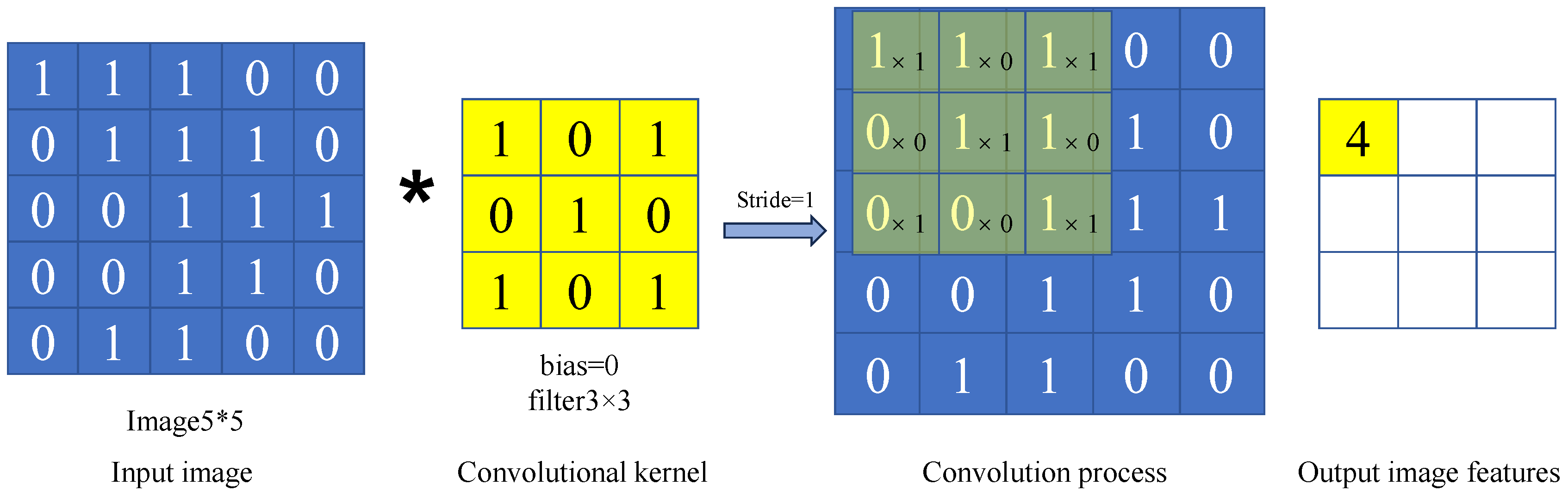
The convolutional layer serves as the cornerstone of a convolutional neural network, which consists of multiple well-designed convolutional kernels. Convolutional kernels are used for the extraction and recognition of significant features in an image, and each convolutional kernel is responsible for detecting specific features in the input data. The two-dimensional convolutional kernel operation process is shown in Figure 1.

Figure 1.
Convolutional kernel arithmetic process.
The convolution operation slides a convolution kernel over the input data to generate a series of Feature Maps, each representing the intensity distribution of a detected feature in the input data. These feature mappings can contain higher-level feature information such as edges, textures, or more abstract features. It helps the network to learn more complex and abstract representations, thus improving the performance and generalization of the network. The mathematical model is described as
where wil denotes the weight in the convolution kernel i in layer l. bil denotes the bias of the convolution kernel i in layer l. xl(j) denotes the input of neuron j in layer l. xil+1(j) denotes the output of neuron j in the layer.
Convolutional layers usually also include an activation function layer, such as ReLU, for introducing nonlinearities. Its function expression is given as
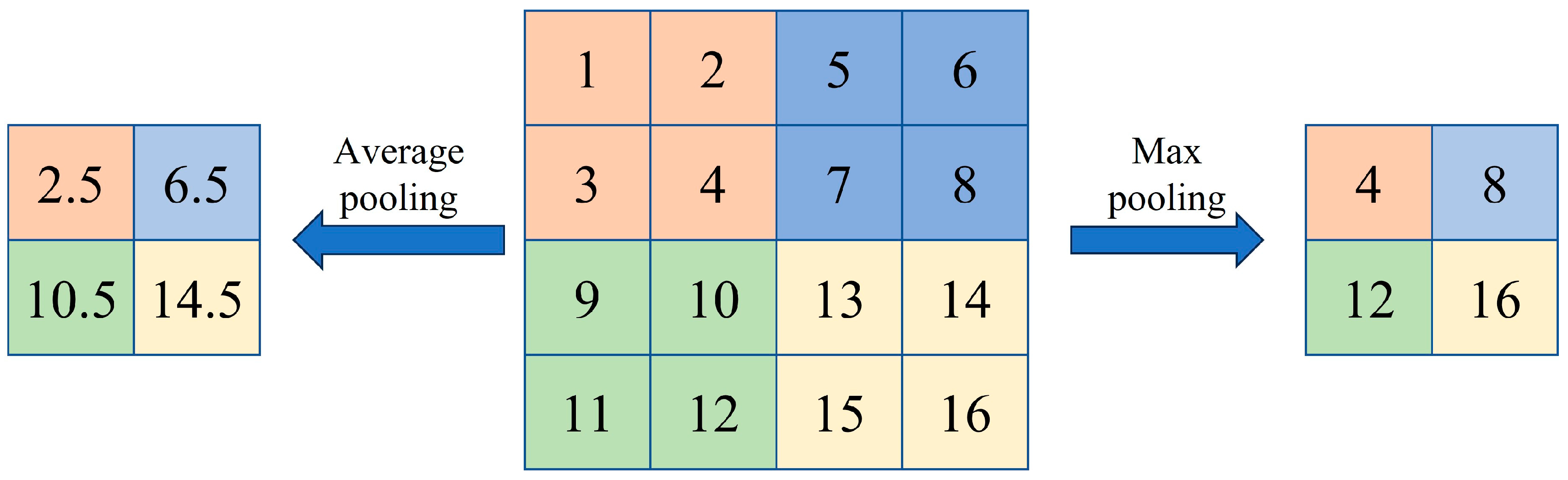
The pooling layer is used to reduce the size of the feature map and retain important information to reduce the dimensionality of the data. The pooling layer not only reduces the amount of computation but also has some translation invariance to better handle the spatial information of the input data, which helps the network to learn a more robust and generalized feature representation. The two main operations of the pooling layer are shown in Figure 2: average pooling and maximum pooling.
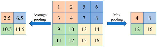
Figure 2.
Maximum and average pooling.
Average Pooling: Take the average of the features in the pooled kernel as output. The expression for average pooling is as
where qul(ij) is the output of channel u of neuron ij in layer l, the size of the pooling kernel is s, and pul+1 is the output of channel u in layer l+1 of the pooling layer.
Maximum pooling takes the maximum value in the sensory field as the output, with the formula
where qul(ij) is the output of channel u of neuron ij in layer l, the size of the pooling kernel is s, and the step size is v. pul+1 is the output of channel u at layer l+1 in the pooling layer.
The main function of the fully connected layer is to convert the feature map output from the pooling layer into a one-dimensional feature vector and pass the resulting feature vector to the subsequent neural network layer for further processing. In the structure of fully connected layers, each neuron plays the role of integrating information. The neuron takes the output data from all the neurons in the previous layer as input and receives them. Then, a weighting calculation is performed based on the preset weights of the neurons. Finally, the output is generated through an activation function.
Through this connection, the fully connected layer can efficiently integrate the information of fault features learned from the previous layer. At a higher level, the fully connected layer abstracts and recombines these features. Doing so enables a higher level of classification or identification of the input data. Finally, complex associations between the input features and the final output are established by learning and adjusting the weighting parameters. The fully connected layer is typically used for the final classification or regression task.
The output layer is responsible for generating the output of the model. Depending on the task requirements, Convolutional Neural Networks (CNNs) can be employed for binary classification problems (with Sigmoid activation functions), multi-class classification problems (with Softmax activation functions), or regression problems (without specific activation functions).
When constructing a CNN, its structure is usually designed as a hierarchical structure of multiple convolutional layers, pooling layers, and fully-connected layers stacked alternately to form a multi-layered complex architecture. This architecture enables CNNs to gradually extract more and more abstract feature representations from the original input data, which are ultimately used to realize various complex tasks, such as image recognition and target detection.
During the training process, the network is progressively tuned and optimized with backpropagation algorithms to maximize the network performance at each layer. Convolutional neural networks can also use techniques such as batch normalization and dropout to improve their stability and generalization. In conclusion, convolutional neural networks achieve automatic learning and extraction of features from input data with the help of components such as convolutional operations, pooling operations, and fully connected layers.
SqueezeNet for fault diagnosis at the fluid end of the drilling pump consists of a convolutional layer, a global average pooling layer, multiple Fire Modules (containing Squeeze and Expand layers), multiple maximal pooling layers, a fully-connected layer, an output layer, and the structural parameters of the SqueezeNet model are shown in Table 1. In this paper, a SqueezeNet is employed, with the structural parameters shown in Table 1.

Table 1.
Structure parameters of SqueezeNet model.
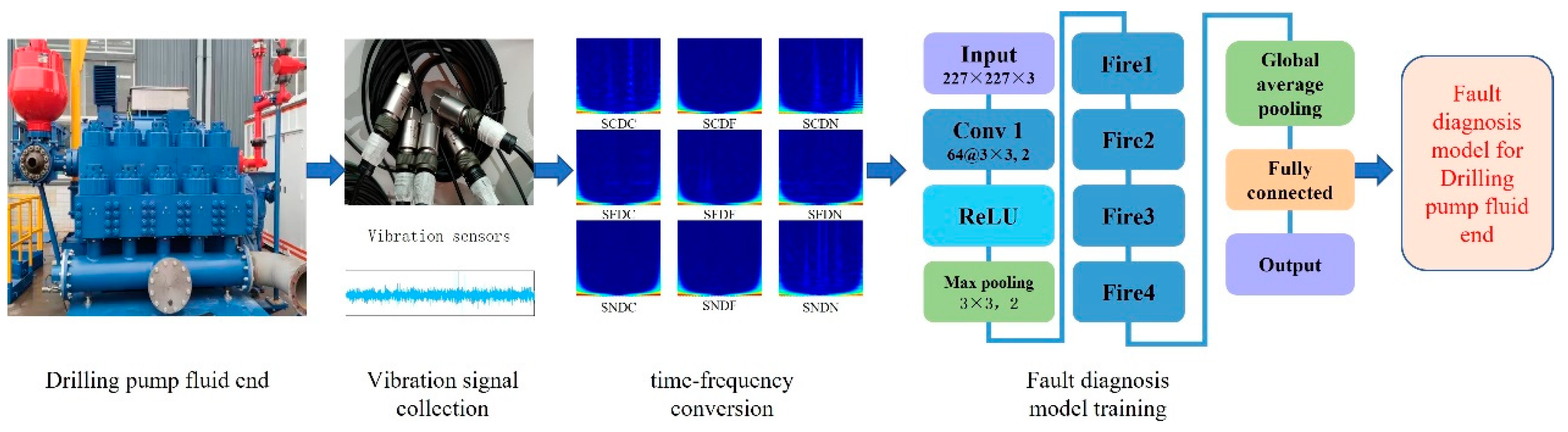
The structural type of the SqueezeNet model is shown in Figure 3. In the processing flow of the SqueezeNet model, the input image first passes through a convolutional layer for key feature extraction. This convolutional layer performs sliding operations on the input image through a set of well-designed convolutional kernels (also commonly known as filters), using convolutional operations to effectively capture and refine the core feature information in the image.
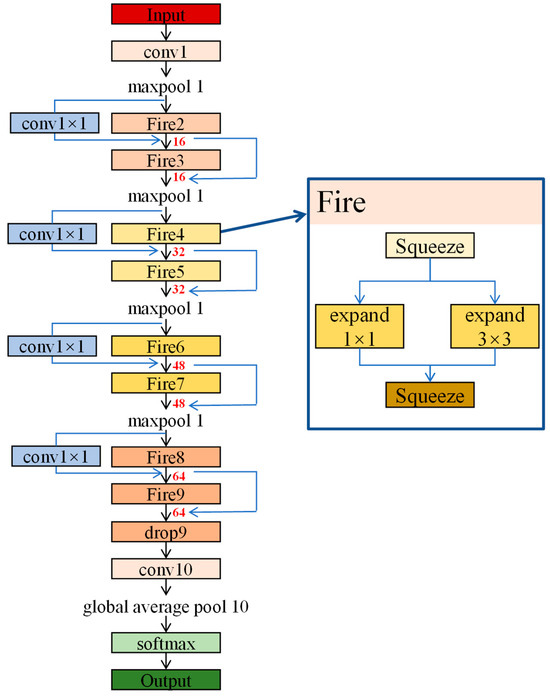
Figure 3.
Structure of SqueezeNet.
Feature compression is then performed in the Squeeze layer of Fire Modules, and the compressed feature maps are used in the Expand layer of Fire Modules using 1 × 1 and 3 × 3 convolution kernels to increase the number of channels (or called extensions), and a mix of convolution kernels of different sizes allows for the capture of features at different scales.
By stacking multiple Fire Modules, SqueezeNet can gradually extract higher-level features. Between Fire Modules, SqueezeNet uses a pooling layer to reduce the spatial size of the feature map.
The pooling operation reduces the resolution of the feature map by selecting the maximum value within each pooling window while retaining the most important information.
By combining and stacking these layers, SqueezeNet can extract rich features from the input image and ultimately convert these features into outputs in the form of category probabilities or other forms of outputs through fully connected layers.
3. The Proposed Approach and Experimental Design
3.1. The Process of the Fault Diagnosis Method of Drilling Pump Fluid End
The fault diagnosis method based on time-frequency analysis and convolutional neural network for the fluid end of the drilling pump mainly includes three processes: fault data acquisition of the drilling pump’s fluid end, data pre-processing, SqueezeNet model training and parameter optimization, and its fault diagnosis process is shown in Figure 4.
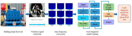
Figure 4.
The process of the fault diagnosis method.
- (1)
- Acquisition of fault data from the fluid end of the drilling pump: Vibration fault signals are collected by acceleration sensors installed at the fluid end of the drilling pump as raw status data.
- (2)
- Data preprocessing: the acquired one-dimensional time-domain signal is transformed into a two-dimensional time-frequency image by continuous wavelet transform method to get the distribution of the signal in time and frequency. Then, a library of time-frequency feature samples is constructed and divided into a train set and a test set according to the ratio of 2:8.
- (3)
- SqueezeNet model training and parameter optimization: The SqueezeNet model was constructed by changing the number of output channels of the model to 9 and initializing all other model parameters randomly. Subsequently, during model training, the data from the training set is provided as input to the model, and the corresponding fault labels are taken as the desired output of the model.
3.2. Data Acquisition for Experiments
Due to the role of alternating pressure load, the suction and discharge valves of the fluid end of the drilling pump are often damaged. In view of this phenomenon, this paper carries out troubleshooting experiments on the suction and discharge valves of the fluid end of the drilling pump. The experiment will be the failure of these two valves into three states, respectively: the normal state, as shown in Figure 5a; the slightly damaged state, as shown in Figure 5b; and the serious damage state, as shown in Figure 5c.
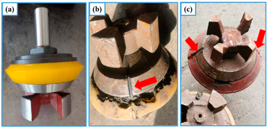
Figure 5.
The three states of the valves. (a) Normal state (b) Minor damage (c) Severe damage.
In the experiments, the pump was operated under different fault states, and 9 fault types at the fluid end of the drilling pump were obtained, as shown in Table 2.
Table 2.
Nine types of faults.
As shown in the figure, the five-cylinder drilling pump used in this experiment has a rated power of 2400 HP, a maximum pump stroke of 188 SPM, and external dimensions of 8076 × 3155 × 2910 mm. The vibration data of the mechanical equipment is an important piece of information for evaluating the operational status of the equipment, predicting failures, and performing maintenance.
Normally, through the observation of the vibration signal amplitude, frequency, phase, and waveform characteristics of the information, you can determine whether the mechanical equipment is in normal operation or there is a fault, and further judge the type of fault and determine the location of the fault and the cause of the occurrence of the fault.
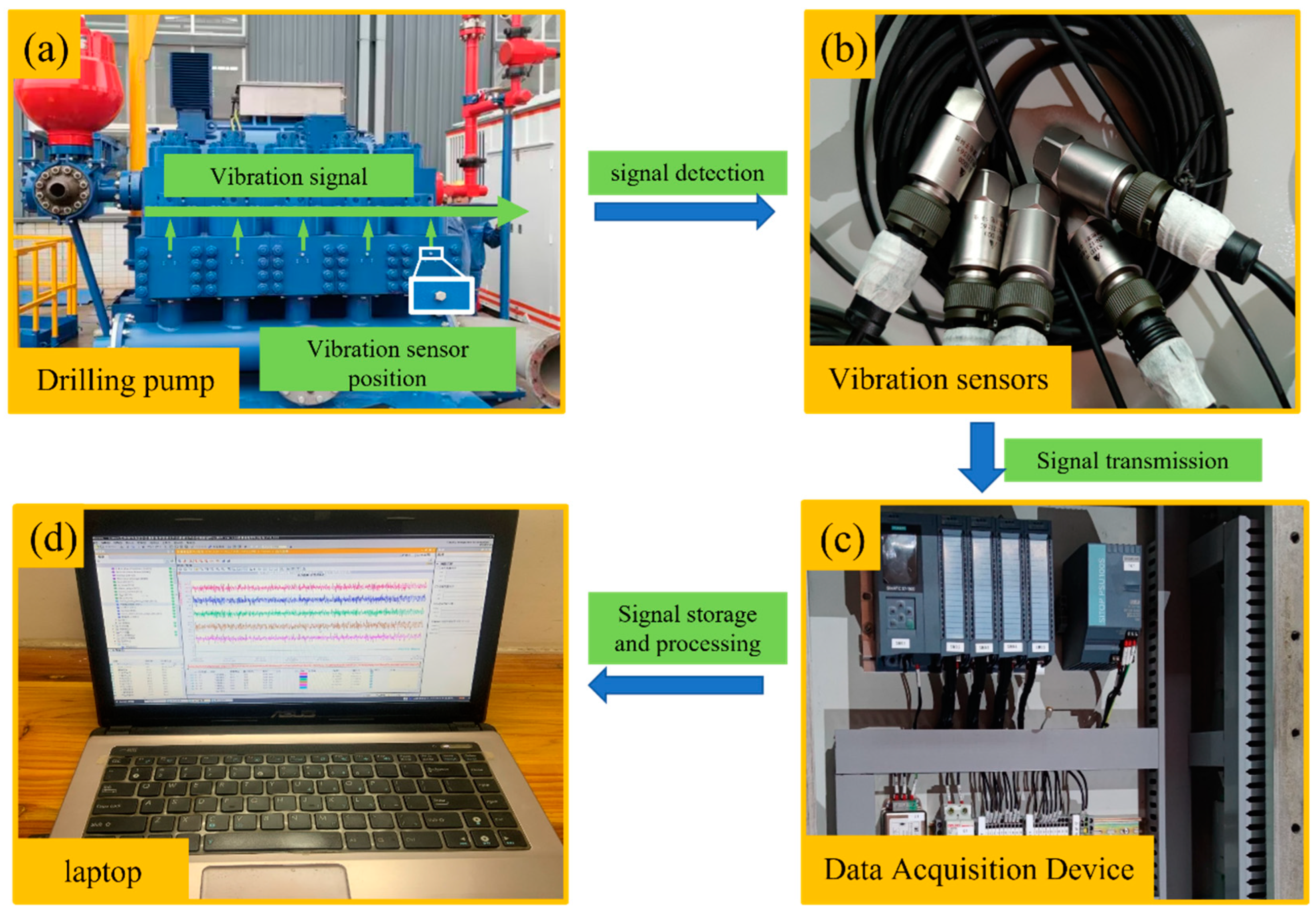
As shown in Figure 6a, this experiment installs acceleration sensors S31D20 for obtaining vibration fault signals on five suction valve boxes at the fluid end of the drilling pump, as shown in Figure 6b. Figure 6c shows that the device is acquired through a PLC. The data is stored and processed through a computer, as shown in Figure 6d.
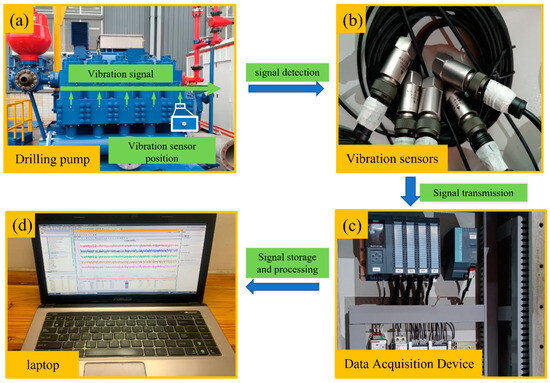
Figure 6.
Experimental equipment and data collection process.
PLC Signal Acquisition and Storage is the process of acquiring signals from various sensors and actuators from a Programmable Logic Controller (PLC) and storing them in an appropriate location. Firstly, acceleration sensors are deployed at the fluid end of the drilling pump to capture the vibration fault signals, followed by connecting the sensors to the controller to ensure that the data can be transmitted and captured properly.
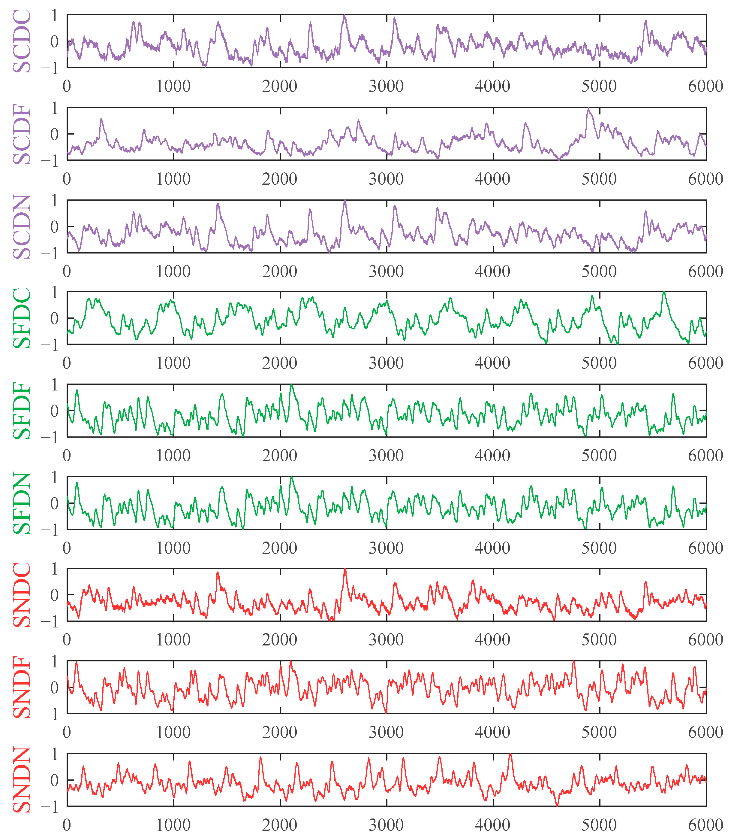
The acquired signals are then processed, for example, filtered, calibrated, or formatted to ensure their accuracy and usability. Finally, the processed fault signals or raw data are stored using the PLC’s internal memory, an external storage device (such as an SD card or USB memory), or a cloud database. As shown in Figure 7 or nine types of 1D fault vibration signals.
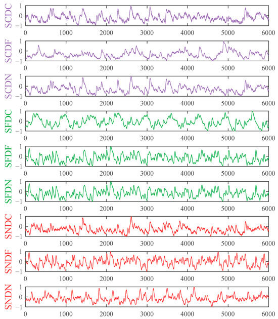
Figure 7.
Nine types of faults vibration signals.
3.3. Fault Data Pre-Processing on the Drilling Pump Fluid End
The experimental data were segmented into 1-s lengths. At the same time, to enlarge the sample size and to prevent the correlation between the fault diagnosis results and the phase of the experimental data, a randomly selected point within 10 percent of the endpoint of the previous data is used as the starting point of the next data. There are 2000 data items for each type of fault under multiple operating conditions, and each data item contains 1000 sample points of vibration signals. The whole dataset contains a total of 18,000 data.
After randomly assigning the data for each type of fault, 80% is selected as the training set with 1600 data for each type of fault, totaling 14,400. The remaining 20% is the test set with 400 pieces of data for each type of fault, totaling 3600 pieces.
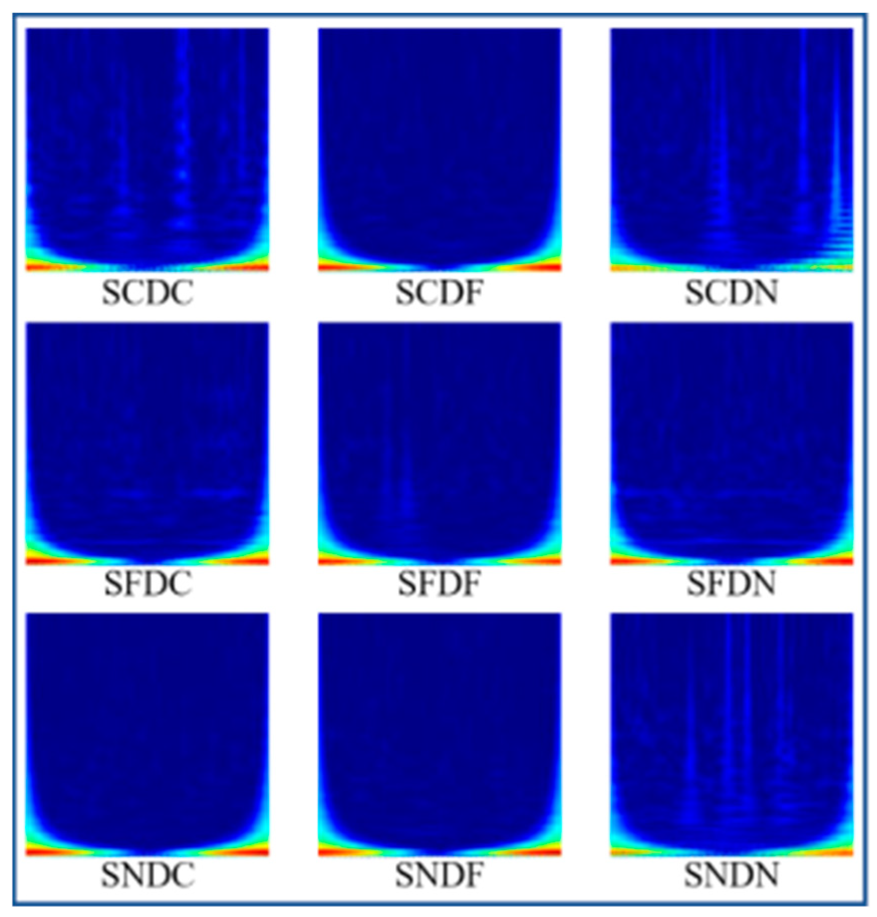
As shown in Figure 8 all the fault data are transformed into a two-dimensional time-frequency map with a size of 227 × 227 pixels by CWT. The horizontal axis of the time-frequency diagram represents time, the vertical axis represents frequency, and the color represents amplitude, obtaining the distribution of the signal in the two dimensions of time and frequency. It constitutes the fault diagnosis image dataset.
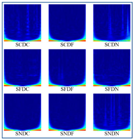
Figure 8.
Time-frequency diagrams for nine fault types.
4. Results and Discussions
4.1. Determination of Hyperparameters
Hyperparameters are one of the key factors affecting model performance. Optimizer and learning rate are the key hyperparameters affecting the model performance. Therefore, a study on the law of influence of optimizer and learning rate on model performance was carried out, and the best hyperparameters were identified. The optimizer is the key to deep neural networks. It ensures the model achieves the best fit on the training data by adjusting the model parameters to optimize the loss function.
During the training process, the selection of appropriate optimizers and their proper adjustment play a crucial role in improving the convergence efficiency of training and the model’s effectiveness. In this paper, we mainly investigate the effects of three optimizers on the model performance, respectively: root mean square backpropagation (RMSprop), Adaptive Moment Estimation (i.e., Adam), and Stochastic Gradient Descent with momentum (i.e., SGDM).
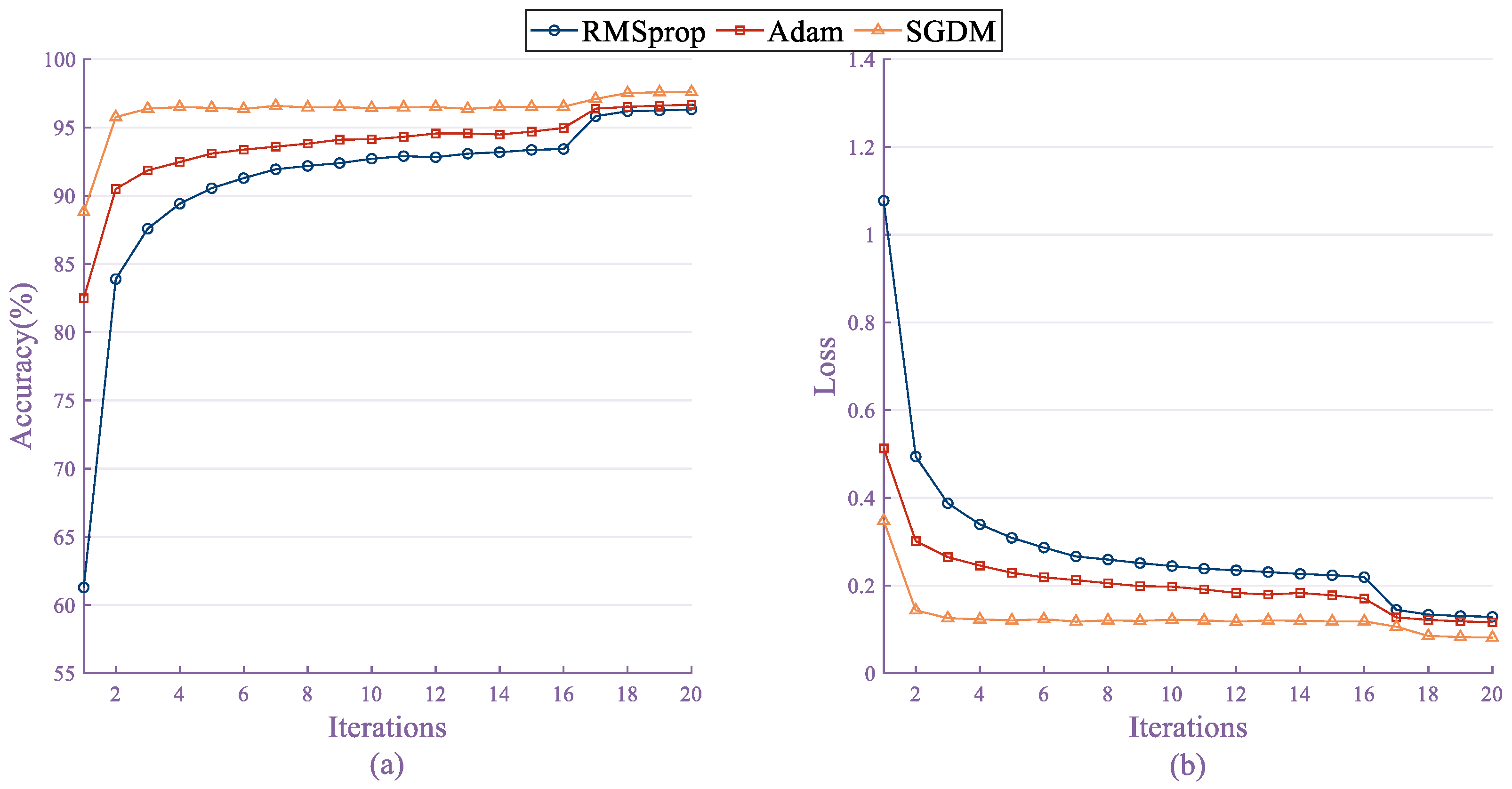
The above three optimizers are used to train the fluid end fault diagnosis model, respectively. The training accuracies of each iteration are shown in Figure 9a, and the training losses of each iteration are shown in Figure 9b. When keeping the rest of the hyperparameters consistent, they all have good training results: RMSprop: 96.12% accuracy with a loss rate of 0.15; Adam: 96.46% accuracy with a loss rate of 0.13; and SGDM: 97.17% accuracy with a loss rate of 0.1.
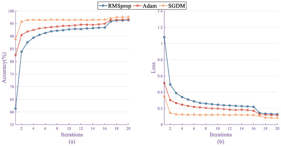
Figure 9.
Training history graph of three types of optimizers.
By analyzing the training history plots of these three types of optimizers, it is concluded that the SGDM optimizer has higher fault diagnosis accuracy and smoother transitions during model training. Compared to the other two optimizers, the SGDM shows superior stability and convergence at different stages of model training, demonstrating the applicability of the SGDM optimizer under the SqueezeNet model.
Experiments comparing the three optimizers, RMSprop, Adam, and SGDM, under the SqueezeNet model show that the SGDM optimizer performs the most superior in terms of fault diagnosis accuracy and is the preferred optimizer for the SqueezeNet model for the fault diagnosis task, keeping the rest of the hyper-parameters consistent.
Gradient descent is an optimization algorithm that updates the parameters by calculating the gradient to minimize the loss function. It uses an iterative mechanism to gradually adjust the parameter values in the inverse direction of the gradient of the loss function over the parameters to approximate the optimal solution.
In each iteration of the model update, the gradient descent method obtains the gradient information by calculating the partial derivatives of the loss function concerning the model parameters and, based on the gradient information, gradually adjusts the values of the parameters along the direction in which the loss function decreases the fastest (namely, the direction of the negative gradient) to achieve the minimization of the loss function. This iterative process continues until the loss function converges or a preset stopping condition is met.
The performance of the gradient descent method is highly dependent on the fine-tuning of the parameters, and the learning rate is one of the most critical hyperparameters. The learning rate is used to adjust the magnitude of the pace at each parameter update, which determines how much the parameter moves in the parameter space.
If the learning rate is set too low, the convergence speed of the model will be significantly reduced, resulting in the training process becoming slower and requiring more iterations to gradually approach the optimal solution; on the contrary, if the learning rate is set too high, the optimization process may fluctuate in the region close to the optimal solution, and may even miss the optimal solution, resulting in the model failing to converge stably.
Therefore, during model training, a reasonable selection and adjustment of the learning rate is crucial to ensure the effectiveness and efficiency of the gradient descent method. Usually, an appropriate learning rate needs to be selected based on the specific problem and data characteristics. The optimal learning rate can be determined through cross-validation or empirical-based adjustment.
A common practice is to use optimization algorithms with adaptive learning rates, such as SGD, RMSprop, and Adam, which are capable of dynamically adjusting the learning rate according to the gradient of the parameters to improve the efficiency and stability of optimization.
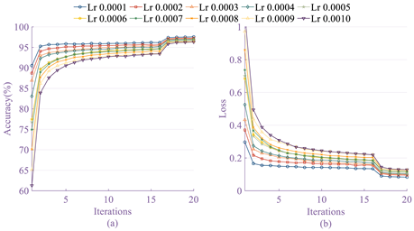
Therefore, choosing an appropriate learning rate is crucial for the successful application of gradient descent for model training. In this experiment, the learning rate is controlled at [0.0001, 0.0010], i.e., the learning rate is set to 0.0001, 0.0002, 0.0003, 0.0004, 0.0005, 0.0006, 0.0007, 0.0008, 0.0009, 0.0010, respectively; the optimal parameters of the model are searched for by sequentially increasing the learning rate and the learning rate increases by 0.0001 for each completion of the training rounds. Under the same number of rounds, the SGDM optimizer increases the learning rate by 0.0001 for each completed training.
From the data in Table 3, it can be observed that under the same model architecture, number of training rounds, and optimizer conditions, the change in learning rate has a direct impact on the accuracy of model fault diagnosis. As the learning rate gradually increases from 0.0001, the accuracy of the SGDM optimizer-based model on the fault diagnosis task is the first to decrease and then rebound.
Table 3.
Fault diagnosis accuracy of SGDM optimizer with different learning rates.
When the learning rate is set to 0.0001, the model has the highest fault diagnosis accuracy of 97.77%, verifying that a lower learning rate facilitates the model to learn and fit the laws in the data better. When the learning rate is increased to 0.0008, the model has the lowest fault diagnosis accuracy of 97.18%, indicating that a learning rate that is too large may lead to training oscillations and instability.
By comparing the fault diagnosis accuracies of ten groups of different learning rates under the SGDM optimizer, it is concluded that the learning rate that gives the highest fault diagnosis accuracy for the SqueezeNet model is 0.0001.
4.2. Model Performance Analysis
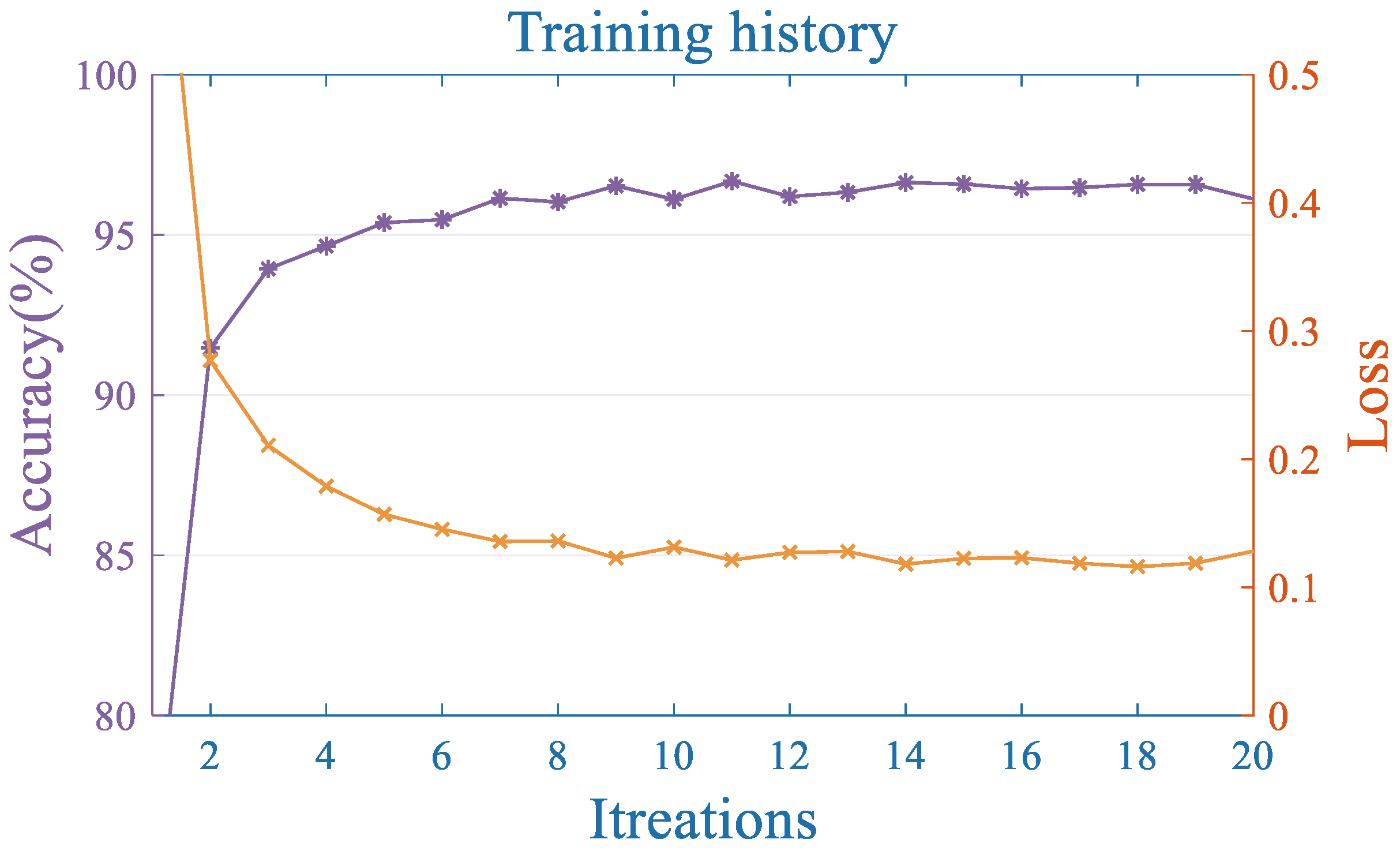
To verify the usefulness of the SqueezeNet model in the fault diagnosis of fluid end of drilling pumps, the fault image dataset generated by CWT is input to SqueezeNet fault diagnosis model and trained according to the best hyperparameters focused on in Section 4.1, and its training history is shown in Figure 10.
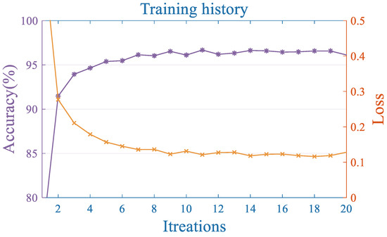
Figure 10.
Training history of fault diagnosis model.
The training accuracy increased steadily as the iterations progressed and was significantly improved to 95% at the 6th iteration, while the loss value converged to 0.1, and the test set accuracy reached 97.77%. The results show that the SqueezeNet fault diagnosis model based on CWT exhibits significant results in the fault diagnosis of the fluid end of the drilling pump.
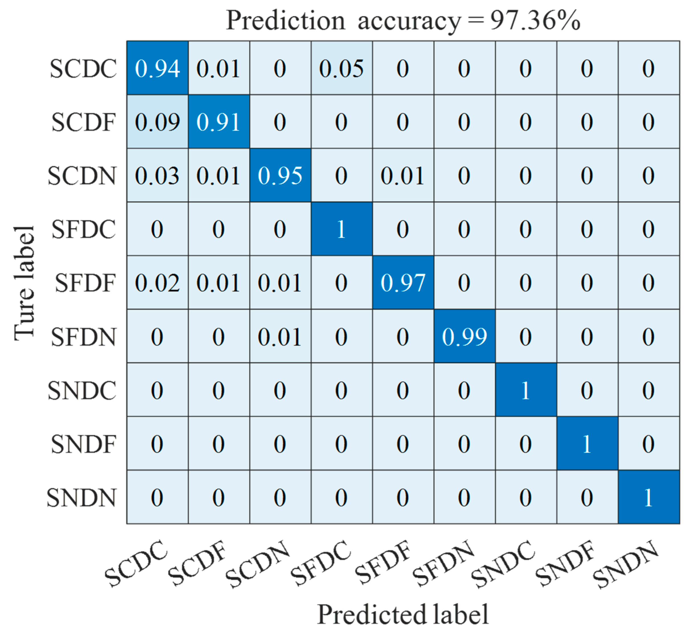
The confusion matrix of the test set is shown in Figure 11. The accuracy of the fault diagnosis model generated by the fault image based on CWT is 97.77%. The five categories of fault diagnosis, SFDC, SFDN, SNDC, SNDF, and SNDN, achieved 100% accuracy. SCDF fault diagnosis had the lowest accuracy of 93% and was severely misclassified as SCDC with a 7% misclassification rate.

Figure 11.
Confusion matrix of fault diagnosis model.
To further demonstrate the superiority of the SqueezeNet model, precision, recall, and F-score are used as metrics to evaluate the performance of the SqueezeNet model. Precision is used to measure the percentage of all instances predicted by the model to be positive samples that are truly positive, reflecting the accuracy of the model in predicting positive samples.
Recall evaluates the proportion of all true positive samples that are correctly identified by the model, reflecting the number of true positive samples that the model can identify. However, there is often a trade-off between precision and recall.
To evaluate the performance of the model in a more comprehensive and balanced way, it is necessary to introduce the F-score to consider both precision and recall dimensions together. The F-score is a reconciled average of precision and recall, which can find a balance between the two, considering both the model’s prediction accuracy and its ability to recognize real positive samples.
The model’s performance is comprehensively evaluated by considering these three metrics, and higher values of these three metrics indicate better model performance. When evaluating the output of the fault diagnosis model, TP (true positive) indicates the number of samples in which a fault actually occurs and is correctly recognized as a fault by the model, TN (True Negative) indicates the number of samples that did not have a fault and were also correctly judged by the model to be fault-free, FP (false positive) indicates the number of samples where the model mistakenly identifies nonfaulty samples as faulty samples, FN (false negative) indicates the number of samples that a fault actually occurs but was not correctly identified by the model as a fault. Based on these definitions, the three metrics can be expressed as,
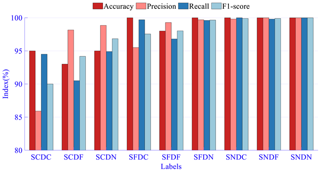
The coefficient β in the F-score is usually set to 1 and called the F1 score. Table 4 compares the accuracy, precision, recall, and F1 scores of nine types of faults at the fluid end based on the SGDM optimizer.
Table 4.
Model performance for each fault.
As can be seen from Table 4, the accuracy of the four-fault categories SFDN, SNDC, SNDF, and SNDN reaches 100%, and the model performance has been significantly improved. The precision and recall of SCDC and SCDF have a large deviation, and the SCDC has a higher recall and lower precision, indicating that the model is too loose, misclassifying many fault samples from non-SCDC categories as this category; SCDF has high precision and low recall, indicating that the model is too conservative and misses many authentic SCDF fault samples. However, after the reconciliation of F1 scores, all nine types of faults are recognized with high accuracy, all above 90%.
In particular, the SqueezeNet model has good recognition performance for the four types of faults: SFDN, SNDC, SNDF, and SNDN. In summary, the SqueezeNet-based fault diagnosis model is superior in identifying the types of faults at the fluid end of the drilling pump.
The receiver operating characteristic (ROC) curve represents the classification performance by balancing selectivity and sensitivity. The horizontal and vertical coordinates of the ROC curve are the false positive rate and the true positive rate, respectively. The closer the ROC curve is to the upper left corner, the higher the area under the curve (AUC) value is, and the better the diagnostic effect.
As shown in Figure 12, the ROC curve and AUC values for each fault of the proposed model are presented, and the effectiveness of the proposed method is proved further.
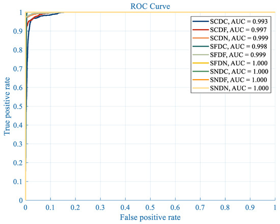
Figure 12.
ROC curves and AUC values of each fault.
T-SNE is a mechanical learning algorithm for the nonlinear dimensionality reduction of high-dimensional data and visualization of the data to facilitate the understanding of the relationships between the data. It maps points in a high-dimensional space to a low-dimensional space using dimensionality reduction techniques while preserving the positional relationships between the original data points as much as possible.
As shown in Figure 13, the Key layer outputs of the test dataset are downscaled to two dimensions by the t-SNE method. Each layer of features was visualized by plotting a clustered scatter plot.
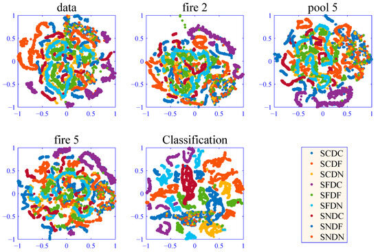
Figure 13.
Visualization of key layer features.
Each point represents fault data in the graph, the color of the point indicates the type of fault, and the distance between the points reflects the distinguishability of the data. The expectation is that faults of the same kind will cluster together. However, in the input layer of the neural network, the mixing of different fault signals makes direct recognition difficult.
With the deepening of the network structure, especially after several well-designed Fire layers, the neural network gradually grasps the core features of various fault signals. These fire layers act as filters to process the input signals in a fine-grained way so that the fault signals, which were difficult to distinguish from each other, are gradually separated.
In the final output layer, the various fault signals are almost totally separated, with only a few overlaps between the two faults, SCDC and SCDF, due to similarity, where a small number of signals are classified as wrong faults. Overall, the neural network demonstrates excellent fault recognition capability.
4.3. Comparative Analysis of Different Fault Diagnosis Methods
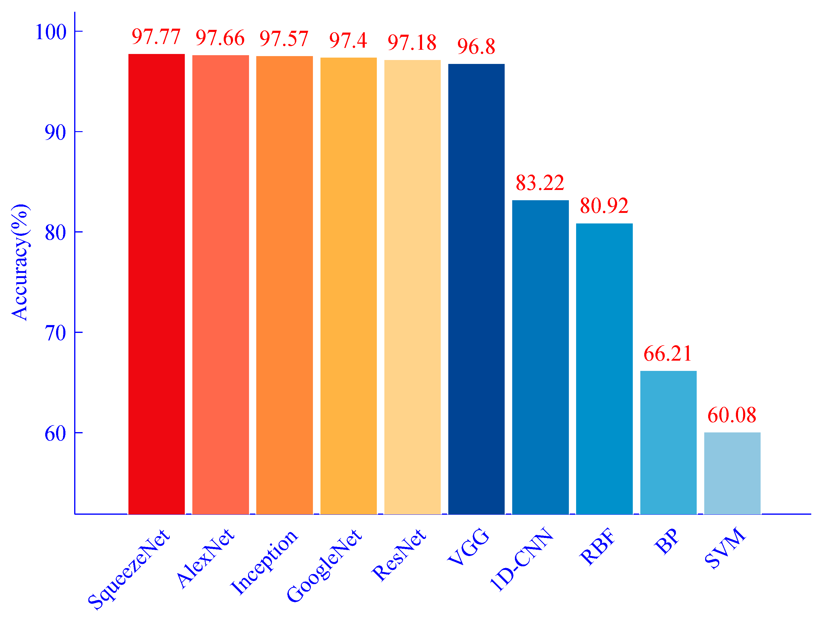
To deeply evaluate the performance of the SqueezeNet fault diagnosis model based on the CWT image dataset proposed in this paper, a comparative study is performed with a series of widely used fault diagnosis methods. These methods cover a variety of deep learning architectures that include Inception, AlexNet, ResNet, GoogleNet, VGG, Radial Basis Neural Networks (RBF), Support Vector Machines (SVMs), BP Neural Networks, and 1D-CNN, and the results of the comparison of these fault diagnosis methods are shown in Figure 14.
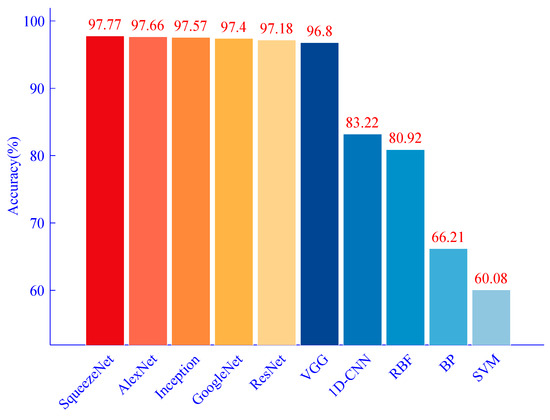
Figure 14.
Comparison of Accuracy of Ten Troubleshooting Methods.
The accuracies of SqueezeNet, AlexNet, Inception, ResNet, GoogleNet, and VGG based on the CWT image dataset are all higher than 90%, reaching 97.77%, 97.66%, 97.57%, 97.4%, 97.18%, and 96.8%, respectively. The accuracy of 1D-CNN and RBF based on time series dataset is 83.22% and 80.92%, respectively.
BP and SVM based on the time series dataset have the lowest diagnostic accuracy of 66.21% and 60.08% and slightly higher than 60%, respectively. The comparative results show that the CWT and SqueezeNet-based methods for diagnosing the faults at the fluid end of the drilling pump have higher accuracy than the other methods.
5. Conclusions
In this paper, a fluid end fault diagnosis method for drilling pumps based on continuous wavelet transform (CWT) and SqueezeNet is proposed. The proposed method can effectively capture the characteristics of fluid end faults to realize the accurate diagnosis of fluid end faults. The study collected fluid end fault data, conducted fault diagnosis experiments, and evaluated the performance of the SqueezeNet fault diagnosis model using four metrics: accuracy, F-score, precision, and recall. The model classification performance was assessed by the ROC curves and AUC values. The learning process of the model is studied through t-SNE. The results proved the effectiveness of the proposed method. At the same time, the study also compares different fault diagnosis methods. This paper’s method is better than other methods, and the comprehensive experimental results prove the effectiveness of the method proposed in this paper.
Author Contributions
Methodology, M.D.; Software, M.D.; Validation, M.D.; Formal analysis, M.D.; Investigation, M.D. and Z.H.; Resources, Z.H.; Data curation, Z.H.; Writing—original draft, M.D.; Writing—review & editing, Z.H. All authors have read and agreed to the published version of the manuscript.
Funding
This work was supported by Nanchong City & Southwest Petroleum University Science and Technology Strategic Cooperation Special Fund (Grant No. 23XNSYSX0130).
Data Availability Statement
The data presented in this study are available on request from the corresponding author.
Conflicts of Interest
The authors declare no conflict of interest.
References
- Chen, Z.; Zhao, W.; Shen, P.; Wang, C.; Jiang, Y. A Fault Diagnosis Method for Ultrasonic Flow Meters Based on KPCA-CLSSA-SVM. Processes 2024, 12, 809. [Google Scholar] [CrossRef]
- Wang, B.; Qiu, W.; Hu, X.; Wang, W. A rolling bearing fault diagnosis technique based on recurrence quantification analysis and Bayesian optimization SVM. Appl. Soft Comput. 2024, 156, 111506. [Google Scholar] [CrossRef]
- Liu, G.; Liu, Y.; Li, H.; Liu, K.; Gao, J.; Zhong, L. Enhancing DGA Transformer Fault Diagnosis Using Data Reconstruction and GD-AHBA-SVM Model. IEEE Trans. Dielectr. Electr. Insul. 2024; early access. [Google Scholar] [CrossRef]
- Wei, Y.; Zhao, J.; Yang, Z.; Wang, P.; Zeng, Z.; Wang, X. Fault detection method for flexible DC grid based on CEEMDAN multiscale entropy and GA-SVM. Electr. Eng. 2024, 1–13. [Google Scholar] [CrossRef]
- Qiu, W.; Wang, B.; Hu, X. Rolling bearing fault diagnosis based on RQA with STD and WOA-SVM. Heliyon 2024, 10, e26141. [Google Scholar] [CrossRef] [PubMed]
- Taibi, A.; Touati, S.; Aomar, L.; Ikhlef, N. Bearing fault diagnosis of induction machines using VMD-DWT and composite multiscale weighted permutation entropy. COMPEL-Int. J. Comput. Math. Electr. Electron. Eng. 2024, 43, 649–668. [Google Scholar] [CrossRef]
- Chang, B.; Zhao, X.; Guo, D.; Zhao, S.; Fei, J. Rolling Bearing Fault Diagnosis Based on Optimized VMD and SSAE. IEEE Access, 2024; early access. [Google Scholar] [CrossRef]
- Sun, Y.; Cao, Y.; Li, P.; Xie, G.; Wen, T.; Su, S. Vibration-Based Fault Diagnosis for Railway Point Machines Using VMD and Multiscale Fluctuation-Based Dispersion Entropy. Chin. J. Electron. 2024, 33, 803–813. [Google Scholar] [CrossRef]
- Yuan, T.; Liang, J.; Zhang, X.; Liang, K.; Feng, L.; Dong, Z. UHVDC transmission line diagnosis method for integrated community energy system based on wavelet analysis. Front. Energy Res. 2024, 12, 1401285. [Google Scholar] [CrossRef]
- Bouaissi, I.; Laib, A.; Rezig, A.; Mellit, M.; Touati, S.; Djerdir, A.; N’diaye, A. Frequency bearing fault detection in non-stationary state operation of induction motors using hybrid approach based on wavelet transforms and pencil matrix. Electr. Eng. 2024, 106, 4397–4413. [Google Scholar] [CrossRef]
- Wang, S.; Tian, J.; Liang, P.; Xu, X.; Yu, Z.; Liu, S.; Zhang, D. Single and simultaneous fault diagnosis of gearbox via wavelet transform and improved deep residual network under imbalanced data. Eng. Appl. Artif. Intell. 2024, 133, 108146. [Google Scholar] [CrossRef]
- Dao, F.; Zeng, Y.; Qian, J. Fault diagnosis of hydro-turbine via the incorporation of bayesian algorithm optimized CNN-LSTM neural network. Energy 2024, 290, 130326. [Google Scholar] [CrossRef]
- Athisayam, A.; Kondal, M. A Smart CEEMDAN, Bessel Transform and CNN-Based Scheme for Compound Gear-Bearing Fault Diagnosis. J. Vib. Eng. Technol. 2024. [Google Scholar] [CrossRef]
- Zhang, J.; Liang, J.; Liu, J. Fault diagnosis in reactor coolant pump with an automatic CNN-based mixed model. Prog. Nucl. Energy 2024, 175, 105294. [Google Scholar] [CrossRef]
- Kim, J.; Choi, M.; Rhee, H.; Park, J.-H.; Yoo, K.-T. Integrity monitoring and fault diagnosis of fuel channel mechanical support for heavy water reactor using CNN. J. Mech. Sci. Technol. 2024, 38, 2773–2779. [Google Scholar] [CrossRef]
- Dash, B.M.; Bouamama, B.O.; Boukerdja, M.; Pekpe, K.M. Bond Graph-CNN based hybrid fault diagnosis with minimum labeled data. Eng. Appl. Artif. Intell. 2024, 131, 107734. [Google Scholar] [CrossRef]
- Gao, J.; Guo, J.; Yuan, F.; Yi, T.; Zhang, F.; Shi, Y.; Meng, Y. An Exploration into the Fault Diagnosis of Analog Circuits Using Enhanced Golden Eagle Optimized 1D-Convolutional Neural Network (CNN) with a Time-Frequency Domain Input and Attention Mechanism. Sensors 2024, 24, 390. [Google Scholar] [CrossRef]
- Patil, A.R.; Buchaiah, S.; Shakya, P. Combined VMD-Morlet Wavelet Filter Based Signal De-noising Approach and Its Applications in Bearing Fault Diagnosis. J. Vib. Eng. Technol. 2024. [Google Scholar] [CrossRef]
- Chang, Y.; Bao, G. Enhancing Rolling Bearing Fault Diagnosis in Motors using the OCSSA-VMD-CNN-BiLSTM Model: A Novel Approach for Fast and Accurate Identification. IEEE Access 2024, 12, 78463–78479. [Google Scholar] [CrossRef]
- Liu, J.; Wan, L.; Xie, F.; Sun, Y.; Wang, X.; Li, D.; Wu, S. Cross-machine deep subdomain adaptation network for wind turbines fault diagnosis. Mech. Syst. Signal Process. 2024, 210, 111151. [Google Scholar] [CrossRef]
- Zhu, Y.; Xie, B.; Wang, A.; Qian, Z. Fault diagnosis of wind turbine gearbox under limited labeled data through temporal predictive and similarity contrast learning embedded with self-attention mechanism. Expert Syst. Appl. 2024, 245, 123080. [Google Scholar] [CrossRef]
- Li, G.; Hu, J.; Ding, Y.; Tang, A.; Ao, J.; Hu, D.; Liu, Y. A novel method for fault diagnosis of fluid end of drilling pump under complex working conditions. Reliab. Eng. Syst. Saf. 2024, 248, 110145. [Google Scholar] [CrossRef]
- Tang, A.; Zhao, W. A Fault Diagnosis Method for Drilling Pump Fluid Ends Based on Time–Frequency Transforms. Processes 2023, 11, 1996. [Google Scholar] [CrossRef]
- Wang, H.; Dai, X.; Shi, L.; Li, M.; Liu, Z.; Wang, R.; Xia, X. Data-Augmentation Based CBAM-ResNet-GCN Method for Unbalance Fault Diagnosis of Rotating Machinery. IEEE Access 2024, 12, 34785–34799. [Google Scholar] [CrossRef]
- Zeng, Z.; Yang, J.; Wei, Y.; Wang, X.; Wang, P. Fault Detection of Flexible DC Distribution Network Based on GAF and Improved Deep Residual Network. J. Electr. Eng. Technol. 2024, 12, 3935–3945. [Google Scholar] [CrossRef]
- Li, C.; Hu, Y.; Jiang, J.; Cui, D. Fault diagnosis of a marine power-generation diesel engine based on the Gramian angular field and a convolutional neural network. J. Zhejiang Univ. Sci. A 2024, 25, 470–482. [Google Scholar] [CrossRef]
- Shen, Q.; Zhang, Z. Fault diagnosis method for bearing based on attention mechanism and multi-scale convolutional neural network. IEEE Access 2024, 12, 12940–12952. [Google Scholar] [CrossRef]
- Liu, X.; Zhang, Z.; Meng, F.; Zhang, Y. Fault diagnosis of wind turbine bearings based on CNN and SSA–ELM. J. Vib. Eng. Technol. 2023, 11, 3929–3945. [Google Scholar] [CrossRef]
- Qin, G.; Zhang, K.; Lai, X.; Zheng, Q.; Ding, G.; Zhao, M.; Zhang, Y. An Adaptive Symmetric Loss in Dynamic Wide-Kernel ResNet for Rotating Machinery Fault Diagnosis Under Noisy Labels. IEEE Trans. Instrum. Meas. 2024, 73, 3517512. [Google Scholar] [CrossRef]
- Wang, T.; Yan, Y.; Yuan, L.; Dong, Y. Real-Time Recognition and Feature Extraction of Stratum Images Based on Deep Learning. Trait. Signal 2023, 40, 2251–2257. [Google Scholar] [CrossRef]
- Shun, Z.; Li, D.; Jiang, H.; Li, J.; Peng, R.; Lin, B.; Liu, Q.; Gong, X.; Zheng, X.; Liu, T. Research on remote sensing image extraction based on deep learning. PeerJ Comput. Sci. 2022, 8, e847. [Google Scholar] [CrossRef]
- Li, C.; Chen, J.; Yang, C.; Yang, J.; Liu, Z.; Davari, P. Convolutional neural network-based transformer fault diagnosis using vibration signals. Sensors 2023, 23, 4781. [Google Scholar] [CrossRef] [PubMed]
- Mian, T.; Choudhary, A.; Fatima, S. Vibration and infrared thermography based multiple fault diagnosis of bearing using deep learning. Nondestruct. Test. Eval. 2023, 38, 275–296. [Google Scholar] [CrossRef]
- Mitra, S.; Koley, C. Early and intelligent bearing fault detection using adaptive superlets. IEEE Sens. J. 2023, 23, 7992–8000. [Google Scholar] [CrossRef]
- Yang, W.; Wang, W.; Wang, X.; Gu, J.; Wang, Z. Fault diagnosis method of a cascaded H-bridge inverter based on a multisource adaptive fusion CNN-transformer. IET Power Electron. 2024; ahead of print. [Google Scholar] [CrossRef]


Disclaimer/Publisher’s Note: The statements, opinions and data contained in all publications are solely those of the individual author(s) and contributor(s) and not of MDPI and/or the editor(s). MDPI and/or the editor(s) disclaim responsibility for any injury to people or property resulting from any ideas, methods, instructions or products referred to in the content. |
© 2024 by the authors. Licensee MDPI, Basel, Switzerland. This article is an open access article distributed under the terms and conditions of the Creative Commons Attribution (CC BY) license (https://creativecommons.org/licenses/by/4.0/).