Investigation of Gas Diffusion Time Dynamics at the Bottom Hole Under Convection–Diffusion Coupling Mechanisms

Abstract

In the study of underground gas diffusion, traditional methods often emphasize diffusion while neglecting the potential impact of convection. This research constructs a coupled model of diffusion and convection to investigate gas transmission characteristics in complex underground environments. The model is validated and calibrated using field measurement data. The results indicate that the coupled model provides a more accurate representation of gas concentration distribution and diffusion time compared to models that consider only diffusion. Furthermore, this study examines the influence of horizontal well inclination angle on gas diffusion time within the framework of convection–diffusion coupling, revealing its underlying variation patterns. This analysis offers a theoretical foundation for enhancing efficiency and safety in oil and gas production as well as related operations. Under the convection–diffusion coupling mechanism, it is found that the inclination angle of horizontal wells significantly affects gas diffusion time; specifically, larger inclination angles result in shorter durations for gas to diffuse from the bottom to the wellhead. Understanding these variation patterns can facilitate optimization in horizontal well design, rational arrangement of production processes, precise prediction of diffusion times, enhancement of existing safety measures, and provision of forward-looking methodologies and technical support for addressing potential risk events within the oil and gas industry. This has substantial practical implications for engineering applications.

1. Introduction

In recent years, the increasing global demand for energy has positioned the extraction and utilization of natural gas as a critical component within the energy supply chain. However, this process is accompanied by potential safety concerns associated with natural gas exploitation. One significant safety hazard in oil field operations is the diffusion of hydrogen sulfide (H₂S) gas [1] within the oil jacket annulus. Hydrogen sulfide is an extremely toxic gas, and its leakage [2] poses serious risks to workers, the environment, and equipment. Although the oil and gas industry has implemented various measures to prevent and mitigate such incidents, achieving a precise understanding and accurate prediction of hydrogen sulfide diffusion processes remains a formidable challenge.

Horizontal well technology has been extensively adopted and plays a crucial role in contemporary oil and gas extraction. Horizontal wells enhance the contact area between the wellbore and the reservoir [3], thereby increasing oil and gas production. This technology has become one of the key methods for developing numerous oil and gas fields. However, during the extraction process, gas diffusion [4] at the bottom of the hole is a significant factor influencing both mining efficiency and safety. The timely and effective diffusion of gas is closely related to pressure distribution within the wellbore, fluid flow characteristics, and potential safety hazards such as gas penetration.

For an extended period, numerous studies have primarily concentrated on the diffusion effects of gas, operating under the assumption that the downhole environment is relatively static or subject to only minor disturbances. The diffusion models developed based on this premise provide a foundational framework for understanding gas transport to a certain extent. However, the actual underground environment is intricate and dynamic; natural convection resulting from pressure and temperature differentials, along with airflow induced by mining activities, collaboratively establish a convective field that cannot be overlooked. This interplay between convection and diffusion significantly alters both the trajectory of gas diffusion and its concentration distribution underground. Hongguang Sun et al. reviewed previous gas transport experiments in laboratory columns and real oil and gas reservoirs, conducted numerical tests and field applications of the convection–diffusion equation (FCDE), and conducted sensitivity analysis and model comparison. The gas dynamics exhibit typical sub-diffusion behavior, which cannot be effectively captured by conventional transport models, while the FCDE model captures the observed gas breakthrough curve, including its obvious positive skew. By establishing and verifying the convection–diffusion equation, it provides a new theoretical model and method for studying gas transport in heterogeneous soil and gas reservoirs, and helps to understand and predict the coupling behavior of gas in complex geological environments more accurately. Relying exclusively on traditional diffusion [5] models can no longer accurately represent the real-world conditions of underground gas dispersion. Consequently, it becomes imperative to investigate the principles governing gas diffusion within a coupled convection–diffusion mechanism. The convection–diffusion coupling process of gas is a complex physical phenomenon, involving the macroscopic flow of gas (convection) and the microscopic molecular movement (diffusion). In practice, the convection and diffusion of gas often exist at the same time and affect each other to form a coupling process. Convection will allow the gas to be transported rapidly over a large area, but also affect the rate and direction of diffusion. A comprehensive examination of the coupling mechanisms between convection and diffusion addresses urgent practical needs while holding substantial scientific significance for enhancing our theoretical understanding of underground gas diffusion as well as improving safety management practices. This study aims to bridge existing research gaps and elucidate a complete physical representation of underground gas diffusion.

2. Basic Theory of Gas Diffusion

Gas diffusion refers to the spontaneous migration of gas molecules from a high-concentration area to a low-concentration area, and its basic theory is mainly based on the following three aspects:

(1) Molecular thermal motion [6]: Gas consists of a large number of molecules, which are constantly in irregular thermal motion. The thermal motion of molecules is the microscopic basis of gas diffusion. The average kinetic energy of molecules is proportional to temperature. The higher the temperature, the more intense the thermal motion of molecules, and the faster the diffusion speed.

(2) Concentration gradient: The driving force of gas diffusion is the concentration gradient. According to Fick’s law, the mass of a gas passing through a unit area in unit time (diffusion flux) is proportional to the concentration gradient. That is, the greater the concentration difference, the faster the diffusion rate. The gas molecules will spread from the place of high concentration to the place of low concentration until the gas concentration is evenly distributed throughout the space.

(3) Diffusion coefficient: The diffusion coefficient [7] is a physical quantity that describes the diffusion capacity of a gas, which is related to factors such as the type of gas, temperature, pressure, and medium. Generally speaking, the diffusion coefficient of small molecule gas is larger and the diffusion speed is faster. With the increase in temperature, the diffusion coefficient increases and diffusion accelerates. As the pressure increases, the diffusion coefficient decreases and diffusion slows down.

2.1. Fick’s First Law

$$J=-D{\displaystyle \frac{\mathit{\partial }C}{\mathit{\partial }x}}$$

(1)

where $\mathrm{J}$ represents the diffusion flux (mol/m²·s), $\mathrm{D}$ denotes the diffusion coefficient (m²/s), $C$ indicates the volume concentration of the diffused substance, and ${\displaystyle \frac{\mathit{\partial }\mathrm{C}}{\mathit{\partial }\mathrm{x}}}$ signifies the concentration gradient (mol/m³).

2.2. Fick’s Second Law

$${\displaystyle \frac{\mathit{\partial }C}{\mathit{\partial }t}}=D{\displaystyle \frac{{\mathit{\partial }}^{2}C}{\mathit{\partial }{x}^2}}$$

(2)

where $C$ represents the volume concentration of the diffused substance (mol/m³), t denotes time (s), $x$ indicates distance (m), and $D$ signifies the diffusion coefficient (m²/s).

2.3. Influencing Factors of Gas Diffusion Coefficient

Under specific conditions, the type of gas (molar mass), along with temperature and pressure, are the primary factors influencing the gas diffusion coefficient.

(1) The Influence of Gas Type

According to Graham’s Law, at a constant temperature, the diffusivity of various gases is inversely proportional to the square root of their molar masses.

$${\displaystyle \frac{D_A}{D_B}}=\sqrt{{\displaystyle \frac{M_B}{M_A}}}$$

(3)

where $D_A$ and $D_B$ represent the diffusivity coefficients of two distinct gases; $M_A$ and $M_B$ denote the molar masses of these two different gases.

(2) The Influence of Temperature

According to the Arrhenius equation, the diffusion coefficient of a gas is:

$$D=D_0\mathit{exp}\left({\displaystyle \frac{-E}{RT}}\right)$$

(4)

where $D$ represents the diffusion coefficient of a gas; $D_0$ denotes the reference diffusion coefficient of the gas; $E$ signifies the diffusion activation energy of the gas; $R$ is the ideal gas constant; and $T$ indicates the absolute temperature. According to Formula (4), when all other factors remain constant, an increase in temperature leads to more vigorous movement of gas molecules. This results in an accelerated diffusion rate and, consequently, a higher diffusion coefficient.

(3) The Influence of Pressure

According to Fuller’s formula, the pressure is inversely related to the diffusion coefficient.

$$D={\displaystyle \frac{1.013\times {10}^{-5}{T}^{1.75}{\left(\frac{1}{M_A}+\frac{1}{M_B}\right)}^{\frac{1}{2}}}{P{\left[{\left(\sum v_A\right)}^{\frac{1}{3}}+{\left(\Sigma v_B\right)}^{\frac{1}{3}}\right]}^2}}$$

(5)

where $D$ represents the diffusion coefficient of binary gases A and B (m²/s), P denotes the total pressure of the gas (KPa), T indicates the temperature of the gas (K), and M_A and M_B are the molar masses of components A and B, respectively (g/mol). Additionally, $\sum v_A$ and $\sum v_B$ refer to the molecular diffusion volumes of components A and B (cm³/mol).

2.4. Chapman–Enskog Theory

The Chapman–Enskog theory posits that the gas diffusion coefficient [8] is directly proportional to the 1.5th power of temperature and inversely proportional to pressure.

$$D_2=D_1\left({\displaystyle \frac{P_1}{P_2}}\right){\left({\displaystyle \frac{T_2}{T_1}}\right)}^{1.5}$$

(6)

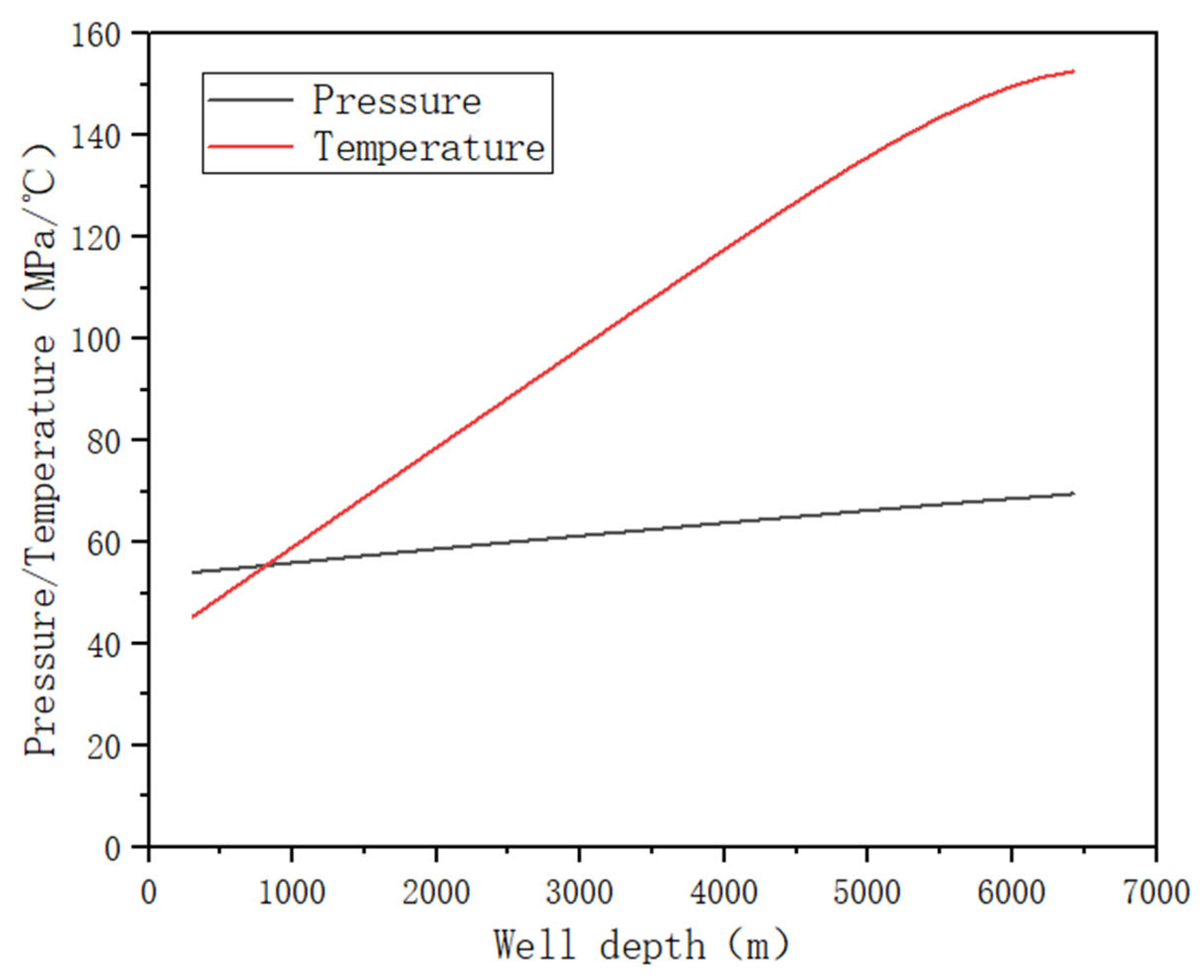
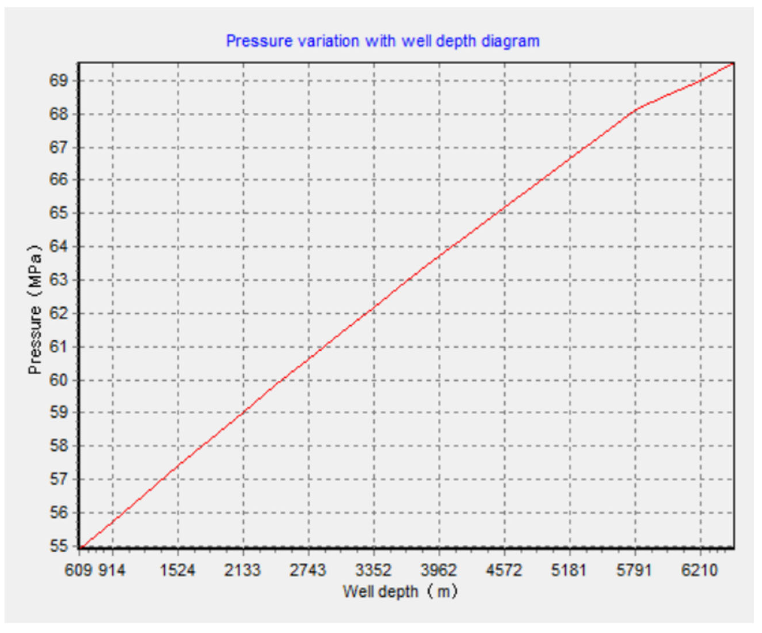
3. Calculation of Pressure and Temperature in the Annular Diffusion Process of Raw Gas Oil Jacket

The research subject of this study is the Yuanba-XX well located in southwest China. The total depth of the well reaches 7000 m. The inner diameter of the casing measures 168.3 mm, while the outer diameter of the tubing is 88.9 mm. A stable supply of raw gas within a 100 m radius from the bottom hole ensures continuity in gas supply. The interval extending from 100 m to 7000 m represents an area where nitrogen (N₂) is distributed, with the oil jacket annulus serving as the diffusion channel for this segment of gas. As the well depth increases to 7000 m, the pressure and temperature at different locations in the wellbore vary greatly, and the gas diffusion velocity is closely related to the temperature and pressure in the oil jacket annulus. Elevated pressure results in gas volume compression and subsequently reduces diffusion speed; conversely, high temperatures enhance molecular movement and facilitate gas diffusion. To accurately predict the time required for gas to diffuse to the wellhead, it is essential to establish a comprehensive gas diffusion model that incorporates fluctuations in wellbore pressure and temperature distribution [9], as shown in Figure 1. Utilizing actual data pertaining to well conditions at this site allows for precise calculations regarding pressure and temperature distributions within the oil jacket annulus region, as shown in Figure 2.

4. Establishment and Solution of Mathematical Model

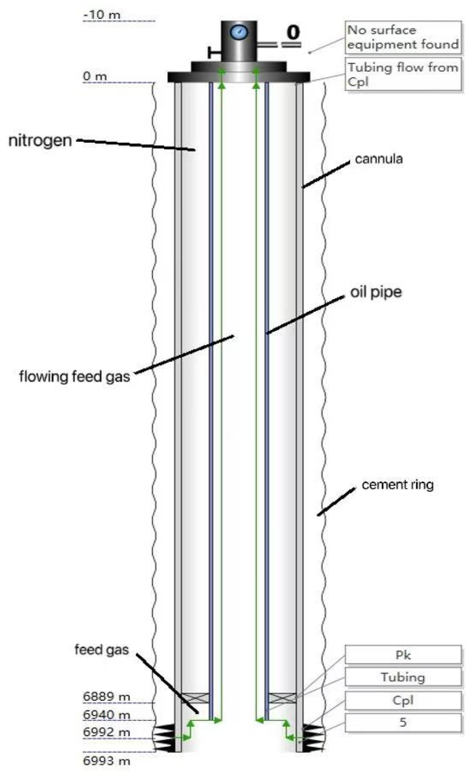
4.1. Well Body Structure

We designed a geometric diagram of a gas well. Initially, the well extends vertically from the ground to a depth of 6000 m. The geometric shape of the well is cylindrical, with a diameter at the wellhead of D = 660 mm. Upon reaching this depth, the gas well begins to tilt at an angle φ = 45 degrees and continues to slope downward for an additional distance of 1000 m. The well structure is shown in Figure 3.

4.2. Pressure and Temperature Processing in Stages

Because pressure and temperature exhibit significant variations at different locations, it is essential to differentiate the pressure and temperature throughout the entire well section in order to obtain accurate pressure and temperature gradients. According to the actual measured data in each section of wellbore, Visual Basic (v6.0) software is used to fit through the least square method, and the relationship expression between temperature and pressure and well depth is obtained. Following the differential analysis of each segment, the results are integrated to provide a comprehensive description of how gas pressure, temperature, and other parameters change with well depth. This allows for further calculations of the diffusion coefficient [10] under varying environmental conditions [11]. The function relation between pressure, temperature, and well depth is fitted by least square method. The relation between pressure and well depth is y = 0.002528x + 53.54451, and the relation between temperature and well depth is y = 0.018221x + 315.3636. By comparing the fitting curve results with the actual measured values, the error is small, the fitting effect is good, and the pressure, temperature, and well depth are linear. The pressure variation curve with well depth is shown in Figure 4. The temperature variation curve with well depth is shown in Figure 5.

4.3. The Convection–Diffusion Coupling Equation Is Established

(1) Definition of Physical Quantities and Directions

In our study of the gas diffusion problem, it is very important to clarify the definition of each physical quantity and direction. We set the gas diffusion direction as the positive direction of the Z-axis, where the inclination Angle θ refers to the angle with the diffusion direction (Z-axis). The acceleration of gravity, g, is going straight down. Since the gravitational component is opposite to the direction of diffusion, the component of gravitational acceleration in the direction of diffusion (Z-axis) g_z = −gcosθ. This clear definition of direction and physical quantity lays the foundation for subsequent analysis.

(2) Consider the sedimentation rate influenced by gravitational forces.

According to Stokes’ law, for spherical gas molecules, the sedimentation velocity in the vertical direction is V_g

$$V_g={\displaystyle \frac{2}{9}}{\displaystyle \frac{r^{2}g\left(\rho -{\rho }_0\right)}{\eta }}$$

(7)

When the wellbore has an inclination Angle θ to the vertical direction, gz = −gcosθ is substituted into (7) to obtain the gravity-induced sedimentation velocity [12] in the Z-axis direction as V_gz

$$V_{gz}=-{\displaystyle \frac{2}{9}}{\displaystyle \frac{r^{2}gcos\theta \left(\rho -{\rho }_0\right)}{\eta }}$$

(8)

where r represents the effective radius of the gas molecule, ρ denotes the density of the gas, ρ₀ signifies the density of the surrounding medium, and η indicates the viscosity of that medium.

(3) Calculate the Flux

a. Diffusion flux

By Fick’s first law, diffusion flux $J_D=-D{\displaystyle \frac{\mathit{\partial }C}{\mathit{\partial }z}}$ where D is the diffusion coefficient and c is the gas concentration.

b. Flux due to gravity

Flux due to gravity $J_g$ = c$V_{gz}$. Substituting (8) gives $J_g$ = c$V_{gz}$ = $-c{\displaystyle \frac{2}{9}}{\displaystyle \frac{r^{2}gcos\theta \left(\rho -{\rho }_0\right)}{\eta }}$.

c. The flux caused by convection

The convection velocity [13] in the z-axis direction is $v_z$. Then, the flux caused by convection $J_{conv}=c{v}_z$.

d. Total flux

The total flux J is the sum of the diffusion flux, the flux due to gravity, and the flux due to convection, namely, $J=J_D+J_g+J_{conv}$.

(4) Derivation of Differential Equations

Conservation of matter according to Fick’s second law ${\displaystyle \frac{\mathit{\partial }c}{\mathit{\partial }t}}=-{\displaystyle \frac{\mathit{\partial }J}{\mathit{\partial }z}}$. That is, the rate of change in the gas concentration per unit time at a certain point is equal to the negative gradient of the flux at that point. By substituting the previous expression for the total flux J into this formula, we obtain

$${\displaystyle \frac{\mathit{\partial }c}{\mathit{\partial }t}}=D{\displaystyle \frac{{\mathit{\partial }}^{2}C}{\mathit{\partial }{z}^2}}+{\displaystyle \frac{\mathit{\partial }}{\mathit{\partial }z}}\left(c{\displaystyle \frac{2}{9}}{\displaystyle \frac{r^{2}gcos\theta \left(\rho -{\rho }_0\right)}{\eta }}\right)-v_z{\displaystyle \frac{\mathit{\partial }C}{\mathit{\partial }z}}$$

(9)

4.4. Solution of Convection–Diffusion Coupling Equation

Let $c\left(z,t\right)=Z\left(z\right)T\left(t\right)$, and bring it into the original equation to obtain:

$$Z\left(z\right)T^{\prime }\left(t\right)=D{Z}^{″}\left(z\right)T\left(t\right)+{\displaystyle \frac{\mathit{\partial }}{\mathit{\partial }z}}\left(Z\left(z\right)T\left(t\right){\displaystyle \frac{2}{9}}{\displaystyle \frac{r^{2}gcos\theta \left(\rho -{\rho }_0\right)}{\eta }}\right)-v_z{Z}^{\prime }\left(z\right)T\left(t\right)$$

Divide both sides by Z(z)T(t) to obtain: ${\displaystyle \frac{T^{\mathrm{\prime }}\left(t\right)}{T\left(t\right)}}=D{\displaystyle \frac{Z^{\mathrm{\prime }\mathrm{\prime }}\left(z\right)}{Z\left(z\right)}}+{\displaystyle \frac{1}{Z\left(z\right)}}{\displaystyle \frac{\mathit{\partial }}{\mathit{\partial }z}}\left(Z\left(z\right){\displaystyle \frac{2}{9}}{\displaystyle \frac{r^{2}gcos\theta \left(\rho -{\rho }_0\right)}{\eta }}\right)-v_z{\displaystyle \frac{Z^{\mathrm{\prime }}\left(z\right)}{Z\left(z\right)}}$.

Let ${\displaystyle \frac{T^{\mathrm{\prime }}\left(t\right)}{T\left(t\right)}}$ = λ (λ is constant); therefore, $T^{\mathrm{\prime }}\left(t\right)$−λ$T\left(t\right)$ = 0 is a first-order ordinary differential equation. The equation of the z part is a second-order linear ordinary differential equation with constant coefficients. The RK45 method, also known as the Runge–Kutta–Fehlberg method, is employed to solve these ordinary differential equations. This adaptive step numerical method estimates and controls error by comparing results from Runge–Kutta methods of different orders at each calculation step, allowing for dynamic adjustment of the step size. After 5000 h (approximately 208 days) of exposure to CH₄ and H₂S the concentration of H₂S gas at the wellhead measures 0.000507 mol/m³, and the change in concentration at the wellhead location over time is shown in Figure 6.

After the diffusion of horizontal wells with varying inclination angles over a period of 5000 h (approximately 208 days), the concentration comparison results of gas at the wellhead are shown in Figure 7.

Because H₂S gas will cause harm to the human body, its safety threshold is 0.0004 mol/m³, so we set the target concentration of H₂S as this threshold in the algorithm, and calculate the time required for H₂S gas to reach the target concentration value at the wellhead. Through Visual Basic software, the results obtained by writing code to solve the equation are shown in Figure 8.

5. Numerical Simulation of Diffusion Process Based on COMSOL

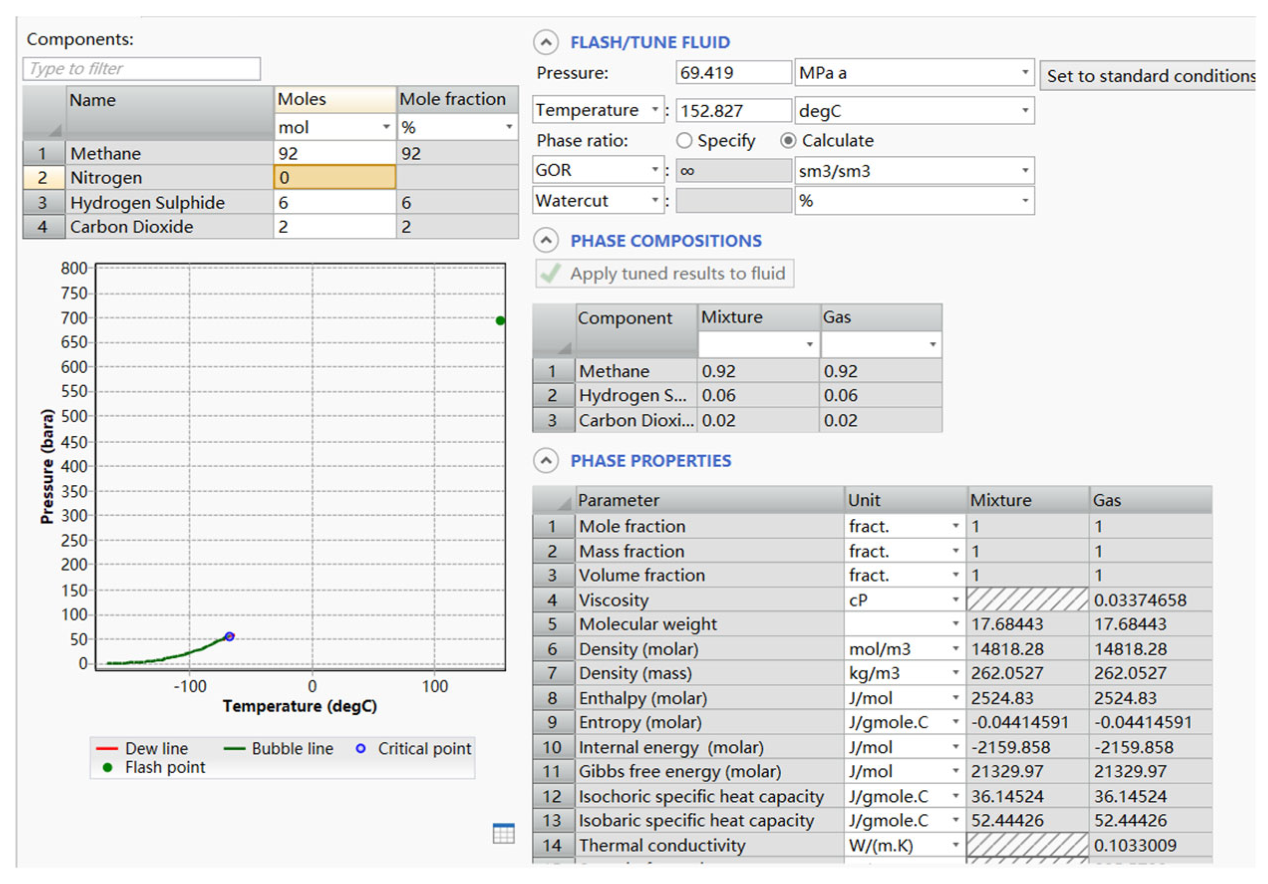
5.1. Phase State Prediction of Annular Diffusion Process of Raw Gas Oil Jacket

In the high-temperature and high-pressure environment [12] we studied, to avoid the possibility of gas liquefaction in the wellbore, we need to analyze and judge the phase state [13] of the gas in the wellbore through pipesim (v2017) software to ensure that the entire process is gaseous. According to the predictions of well fluid dynamics, the preliminary simulation indicated that raw gas composition consisted of 92% CH₄, 6% H₂S, and 2% CO₂. The bottom hole pressure was measured at 69.419 MPa, while the bottom hole temperature reached 152.817 °C. The generated envelope phase diagram is presented in Figure 9. During the process of raw gas diffusion towards the wellhead [14], both pressure and temperature decrease, resulting in a partial mixing with N₂. Consequently, this alters the envelope phase diagram, as illustrated in Figure 10.

As illustrated in Figure 8, at the bottom of the hole, the high concentration of CH₄ (exceeding 90%) results in an envelope phase represented as a curve. The critical point [15] is identified as (5.2 MPa, −75 °C), while the gas state occurs at (69.419 MPa, 152.817 °C). Furthermore, as depicted in Figure 9, both pressure and temperature measurements at the wellhead [16] are lower than those recorded at the bottom of the well. However, upon mixing with some N₂ (an inert gas), the critical point shifts to (5.3 MPa, −101 °C), which remains within a gaseous state.

5.2. Calculation of Diffusion Coefficient

According to Formula (5), the diffusion coefficient of methane (CH₄) and hydrogen sulfide (H₂S) in the binary mixed system [17] under standard conditions is 1.847 × 10^−5 m²/s [18]. At a temperature of 425.76 K and a pressure of 69.549 MPa, the diffusion coefficient for methane (CH₄) and hydrogen sulfide (H₂S) in this binary mixed system remains at 1.847 × 10^−5 m²/s. The diffusion coefficient specifically for methane (CH₄) is measured at 5.541 × 10^−8 m²/s. Given that pressure and temperature within the wellbore can vary significantly, it is essential to calculate the diffusion coefficient in sections to enable a more accurate simulation of the diffusion process.

5.3. Local Diffusion Model

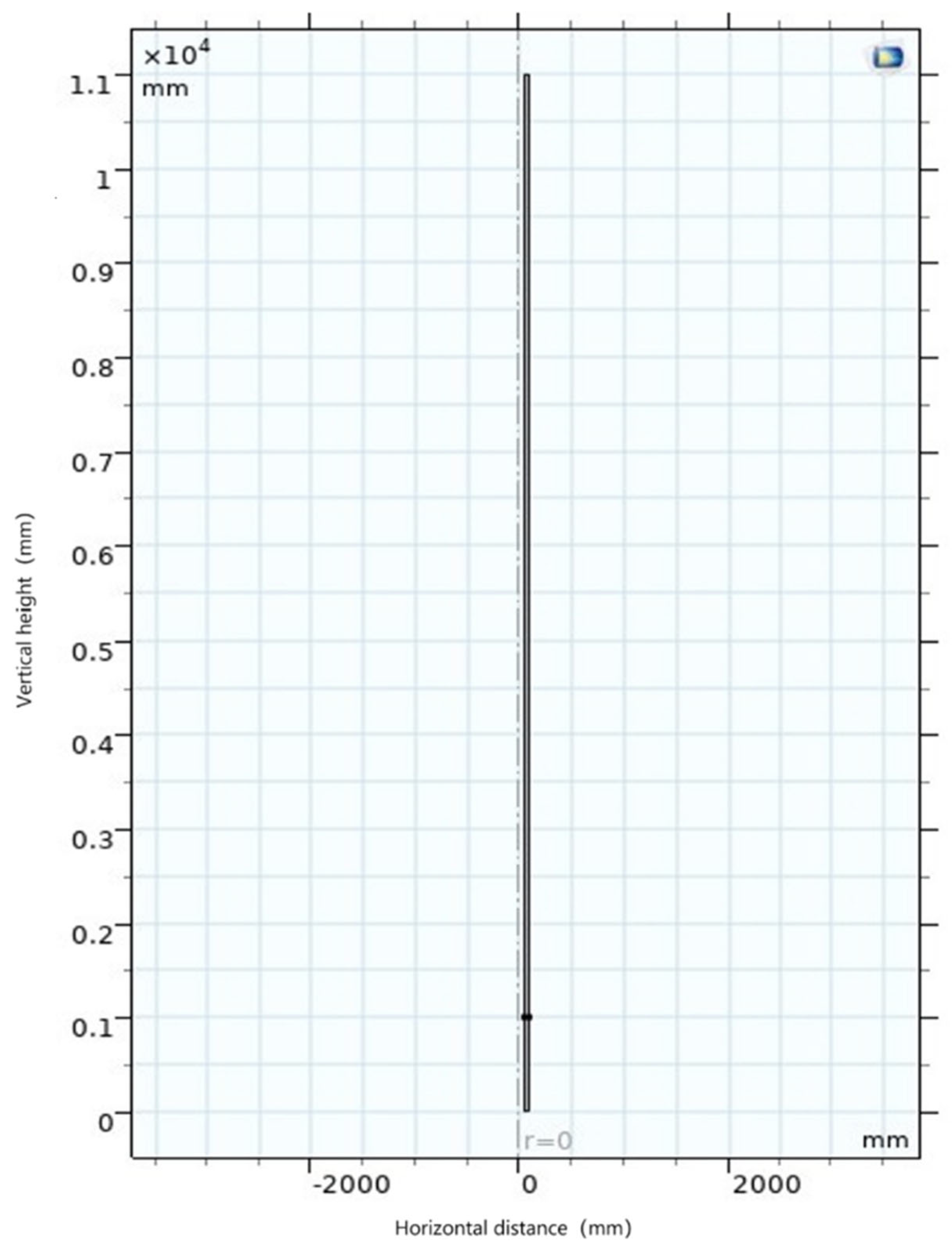
5.3.1. Establishment of Geometric Model

A geometric model measuring 11 m in length was established. To prevent the accumulation of molecules within the boundary layer during the diffusion process, which could impact data selection, the value point for model data was set at 10 m. The 11-meter-long model represents the annular region between the casing and tubing. For computational convenience, this three-dimensional cylindrical model can be simplified into a two-dimensional axisymmetric model for simulation purposes. Additionally, a partial diffusion model can be developed [19], with a total length of 11 m and a designated raw gas section extending from 0 to 1 m at the bottom of the model. This study primarily focuses on hydrogen sulfide (H₂S), setting its concentration at 8%. The methane (CH₄) content is established at 92%, while nitrogen (N₂) constitutes the remainder. The local geometric model is shown in Figure 11.

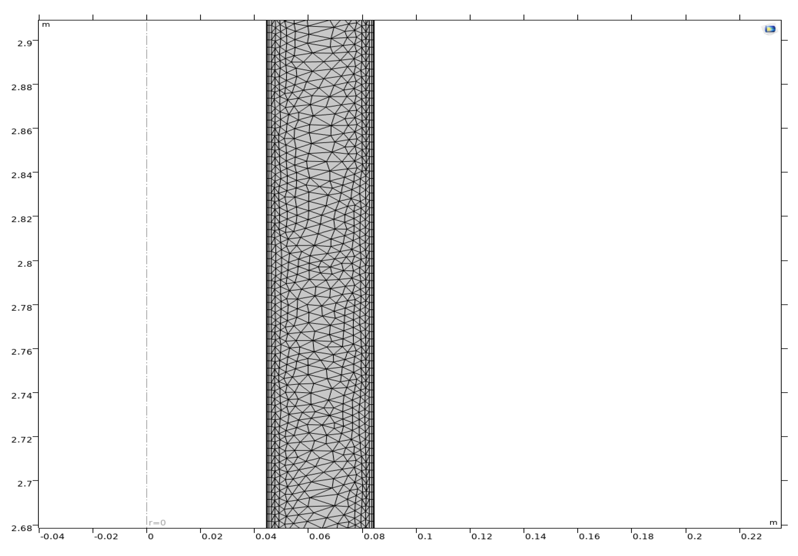
5.3.2. Grid Division

To more effectively capture the changes in geometric details and physical characteristics within the model, enhance the accuracy of simulation results, and accurately simulate the boundary layer, an extremely refined mesh has been employed to better represent these high-gradient regions [20]. This approach is particularly important given the sharp variations in temperature or concentration that occur during the diffusion process. The model grid comprises 373,454 cells, as shown in Figure 12.

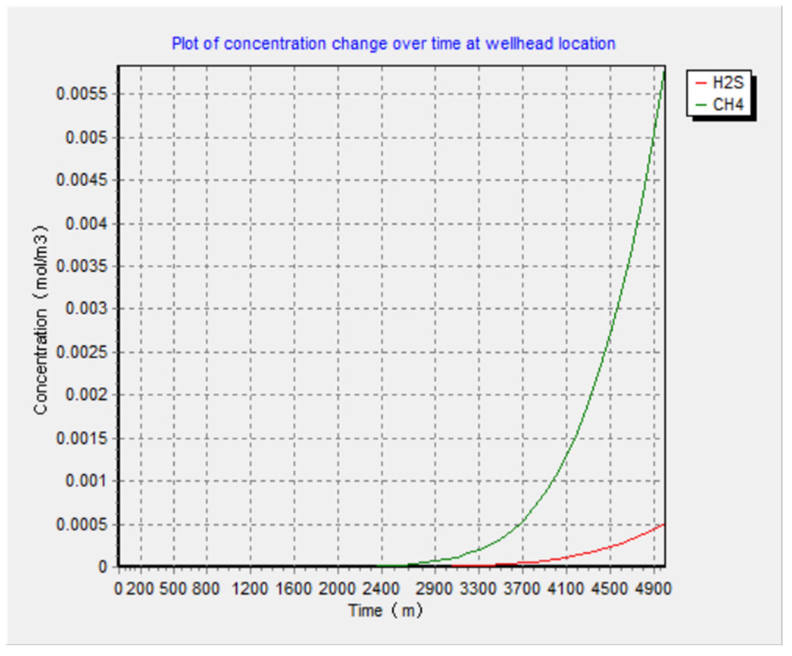
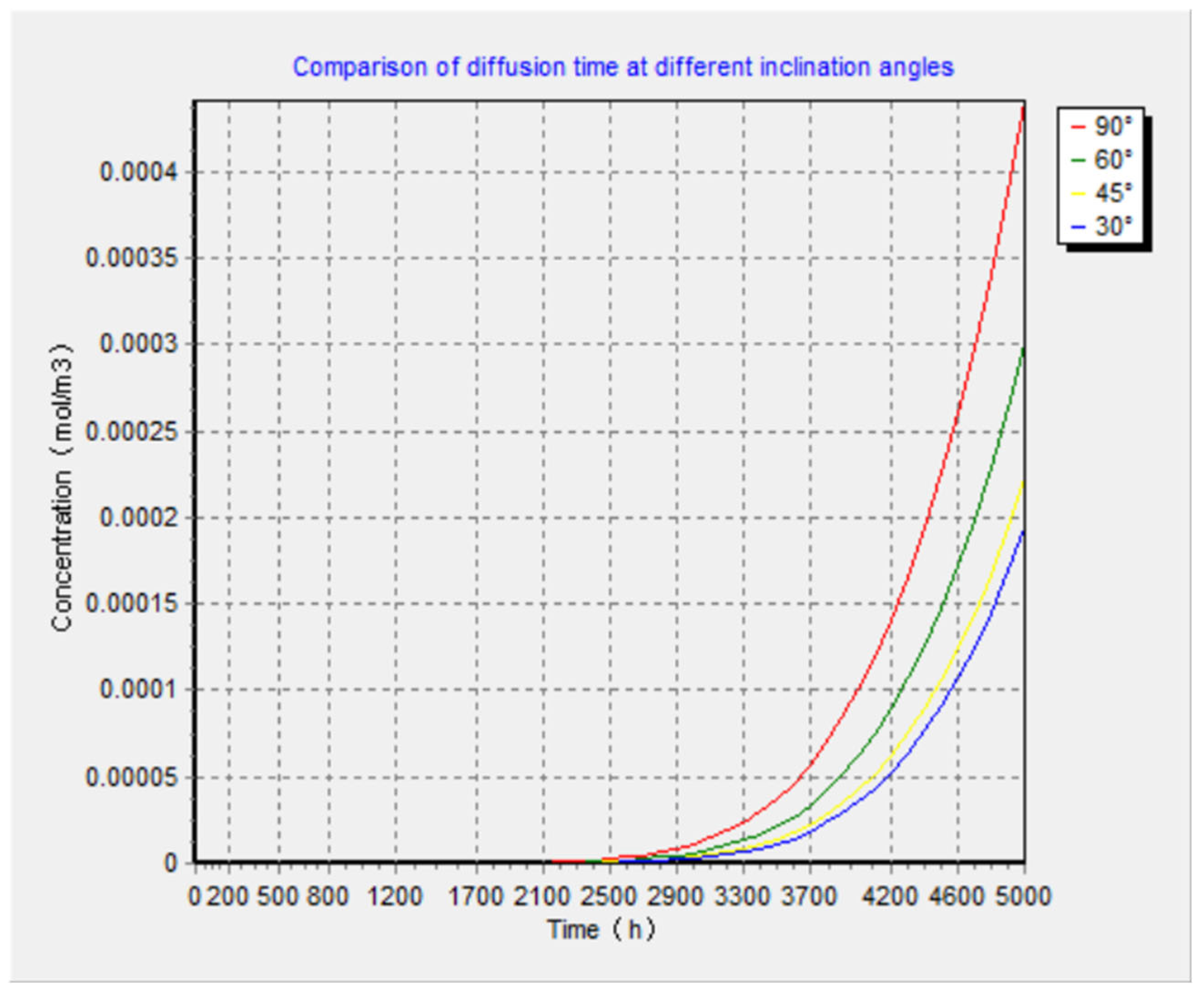
5.3.3. Local Diffusion Model Simulation Results

To enhance the demonstration of the gas diffusion process, a localized model was developed; the initial distribution of H₂S concentration is illustrated in Figure 13a. The model’s diffusion time was established at 3 h (10,800 s), and subsequent calculations were performed; the results are presented in Figure 13b. The CH₄ concentration distribution of the whole section length at 1 h, 30 h, and 100 h after diffusion is shown in Figure 14a–c, respectively.

As illustrated in Figure 13, the stable concentration supply boundary is established at the bottom of the model. Diffusion initiates from a depth of 1 m, while the color remains unchanged at 0 m throughout the entire diffusion process.

5.4. Results of the Complete Diffusion Model

The threshold for harm caused by hydrogen sulfide (H₂S) to the human body is typically expressed in terms of mass concentration [21]. The established threshold value is 10 ppm, equivalent to 0.00044 mol/m³. The safe critical concentration is set at 20 ppm, or 0.00088 mol/m³. To prevent irreversible damage to workers, it is imperative that when the H₂S gas concentration exceeds this safe critical level, nitrogen (N₂) must be re-injected into the wellbore as a precautionary measure [22]. Following analysis and calculations, after approximately 5000 h (or about 208 days) of diffusion, the concentration of H₂S at the wellhead reaches 0.0004513 mol/m³, which surpasses the established threshold value. Therefore, N₂ should be re-injected into the wellbore to ensure effective sealing [23]. The time–concentration changes in H₂S and CH₄ gas diffusion to the wellhead are shown in Figure 15.

6. Conclusions

By solving the mathematical model and physical simulation [24], it can be concluded that under the convection–diffusion coupling mechanism, the inclination angle of horizontal wells (the angle relative to the horizontal direction) significantly influences gas diffusion time at the bottom of the well. Analyses were conducted for inclination angles of 30°, 45°, 60°, and 90°. When the inclination angle of a gas well is small, the time required for gas to diffuse to the wellhead tends to be relatively longer. In this scenario, upward diffusion primarily relies on pressure differences as its driving force [25]. Although gravitational obstruction is minimal (as indicated by a smaller component along the well axis), there are no additional forces aiding in accelerating upward movement. Conversely, when the inclination angle increases—particularly approaching vertical orientation—a notable difference arises between bottom hole pressure and wellhead pressure [26], which becomes a primary driving force facilitating upward gas diffusion. In cases where a gas well’s inclination approaches verticality, pressure difference remains predominant; however, buoyancy forces become more pronounced alongside an increased gravitational component acting along the well axis (in an upward direction). This combination aids in promoting upward spread and accelerates gas diffusion [27]. From an energy perspective, within nearly vertical gas wells, there exists greater potential for converting gravitational potential energy into kinetic energy. As gas ascends toward the wellhead, its gravitational potential energy diminishes; this reduction can partially transform into kinetic energy associated with its upward motion, thereby enhancing diffusion speed [28].

According to the mathematical model convection–diffusion coupling equation established by Visual Basic, it takes 207.7 days for H₂S gas to diffuse to the wellhead, while the diffusion time obtained by COMSOL (v6.3) simulation software is 5000 h (about 208.3 days). The two calculation results are basically consistent, which is also consistent with the information measured in the actual production of the oilfield. Given that H₂S is a highly toxic gas, it poses significant risks to human health, particularly affecting the respiratory and nervous systems. Additionally, H₂S is corrosive [29] and can cause damage to downhole and wellhead metal equipment such as tubing, casing, and trees. In light of these concerns, we recommend implementing a nitrogen re-injection strategy on a 200-day cycle. This approach not only aims to mitigate casualties resulting from H₂S leakage [30], but also effectively reduces the risk of equipment damage. Furthermore, it extends the service life of critical infrastructure while minimizing production interruptions and maintenance costs associated with equipment failures. Ultimately, this strategy contributes to safeguarding the ecological environment surrounding oil and gas fields.

References

1. Zhi, S.J.; Xu, H.F.; Liu, L.Q.; Xue, S.L.; Peng, S.Y.; Zhang, X.B. Characteristics of small hole leakage and diffusion in hydrogen-doped natural gas High Pressure pipeline. J. Petrochem. Univ. 2024, 37, 25–32. [Google Scholar]
2. Chen, Y.; Zhao, J.H.; Zhang, Z.D. Study on leakage and diffusion characteristics of natural gas pipelines. Pet. Chem. Equip. 2022, 25, 8–10. [Google Scholar]
3. Shedid, S.A.; Zekri, A.Y. Sensitivity analysis of horizontal well productivity under steady-state conditions. In Proceedings of the SPE International Improved Oil Recovery Conference in Asia Pacific, Kuala Lumpur, Malaysia, 8–9 October 2001; SPE: Houston, TX, USA, 2001. SPE-72121-MS. [Google Scholar]
4. Yang, D.D. Offshore Platform Sulfurous Gas Leakage Accident Consequence Chain Prediction and Protection Optimization. Ph.D. Thesis, China University of Petroleum (East China), Dongying, China, 2021. [Google Scholar]
5. Chang, A.; Sun, H.G.; Zheng, C.; Lu, B.; Lu, C.; Ma, R.; Zhang, Y. A time fractional convection–diffusion equation to model gas transport through heterogeneous soil and gas reservoirs. Phys. A Stat. Mech. Appl. 2018, 502, 356–369. [Google Scholar] [CrossRef]
6. Luan, Y.; Huo, F.; Lu, M.; Li, W.; Wu, T. Molecular thermal motion harvester for electricity conversion. APL Mater. 2023, 11, 101118. [Google Scholar] [CrossRef]
7. Liu, A.; Liu, P.; Liu, S. Gas diffusion coefficient estimation of coal: A dimensionless numerical method and its experimental validation. Int. J. Heat Mass Transf. 2020, 162, 120336. [Google Scholar] [CrossRef]
8. Lou, H.; Luo, P.; Xue, P.; Yang, W. Quantitative simulation of influencing factors of natural gas diffusion coefficient. Inn. Mong. Petrochem. Ind. 2012, 38, 5–6. [Google Scholar]
9. Li, L.; Huang, W.; Ji, Y.; Zhou, N.; Wang, Y.; Wang, Z. Gas diffusion coefficient of test equipment development and application. J. Exp. Technol. Manag. 2016, 2, 77–80+86. [Google Scholar]
10. Zhang, L.; Guo, J.Y.; Xie, Z.Y.; Liu, A.G.; Yang, C.L. Analysis on technical details of hydrocarbon gas diffusion coefficient determination in rocks. Pet. Chem. Equip. 2019, 22, 28–31. (In Chinese) [Google Scholar]
11. Liu, Y.H. Research on Leakage Model of Natural Gas Pipeline Containing H2S. Master’s Thesis, Southwest Petroleum University, Chengdu, China, 2018. [Google Scholar]
12. Birch, A.D.; Brown, D.R.; Dodson, M.G.; Swaffield, F. The structure and concentration decay of high pressure jets of natural gas. Combust. Sci. Technol. 1984, 36, 249–261. [Google Scholar] [CrossRef]
13. Su, Y.; Li, J.; Yu, B.; Zhao, Y. Numerical investigation on the leakage and diffusion characteristics of hydrogen-blended natural gas in a domestic kitchen. Renew. Energy 2022, 189, 899–916. [Google Scholar] [CrossRef]
14. Liu, G.D.; Zhao, Z.Y.; Sun, M.L.; Li, J.; Hu, G.Y.; Wang, X.B. A new understanding of the diffusion coefficient of natural gas in rocks. Pet. Explor. Dev. 2012, 39, 559–565. [Google Scholar] [CrossRef]
15. Mi, L.-D.; Jiang, H.Q.; Li, J.J.; Tian, Y. Gas diffusion mechanism of shale reservoir. Daqing Pet. Geol. Dev. 2014, 33, 154–159. [Google Scholar]
16. Etiope, G. Natural Gas Seepage: The Earth’s Hydrocarbon Degassing; Springer International Publishing: Cham, Switzerland, 2015; p. 17. [Google Scholar]
17. Yin, Z.H.; Zhao, X.C.; Liu, Z.D. Development of a measuring device for diffusion coefficient of natural gas. Pet. Instrum. 2014, 28, 19–21+16. [Google Scholar]
18. Wang, C. Laser Measurement System and Simulation of Binary Gas Diffusion Coefficient at High Temperature and Pressure. Master’s Thesis, Huazhong University of Science and Technology, Wuhan, China, 2012. (In Chinese). [Google Scholar]
19. Xu, H.F.; Wang, G.X.; Shi, J.; Lu, L. Binary gas diffusion coefficient of a measuring method. J. Dalian Jiaotong Univ. 2012, 5, 90–92. [Google Scholar]
20. Yang, M.; Huang, S.; Zhao, F.; Sun, H.; Chen, X.; Yang, C. Estimation of gas diffusion coefficient for gas/oil-saturated porous media systems by use of early-time pressure-decay data: An experimental/numerical approach. Phys. Fluids 2024, 36, 107134. [Google Scholar] [CrossRef]
21. Ratnakar, R.R.; Dindoruk, B. The Role of diffusivity in oil and gas industries: Fundamentals, measurement, and correlative techniques. Processes 2022, 10, 1194. [Google Scholar] [CrossRef]
22. Phan, B.K.; Shen, K.H.; Gurnani, R.; Tran, H.; Lively, R.; Ramprasad, R. Gas permeability, diffusivity, and solubility in polymers: Simulation-experiment data fusion and multi-task machine learning. npj Comput. Mater. 2024, 10, 186. [Google Scholar] [CrossRef]
23. Yuan, M.; Jing, Y.; Lanetc, Z.; Zhuravljov, A.; Soleimani, F.; Si, G.; Armstrong, R.T.; Mostaghimi, P. Modelling multicomponent gas diffusion and predicting the concentration-dependent effective diffusion coefficient of coal with application to carbon geo-sequestration. Fuel 2023, 339, 127255. [Google Scholar] [CrossRef]
24. Mao, H.Z. Marine Oil and Gas Production Platform Gas Leakage Diffusion Numerical Simulation and Control Study. Master’s Thesis, Hebei University of Engineering, Handan, China, 2022. [Google Scholar]
25. Shi, Y.X.; Liu, F. Effect analysis of offshore oil platform reconstruction on gas diffusion. China Pet. Chem. Stand. Qual. 2019, 39, 151–152. [Google Scholar]
26. Bird, R.B.; Klingenberg, D.J. Multicomponent diffusion—A brief review. Adv. Water Resour. 2013, 62, 238–242. [Google Scholar] [CrossRef]
27. Qian, X.L.; Yan, X.Y.; Zhao, J.P. Simulation of gas pipeline leakage and diffusion in underground integrated pipeline corridor. China Prod. Saf. Sci. Technol. 2017, 13, 85–89. [Google Scholar]
28. Zhang, B.Y.; Ma, G.Y.; Wang, K.; Huang, M.J.; Chen, S.J. Numerical Analysis of leakage diffusion in Buried Natural Gas Pipeline based on CFD. J. Liaoning Shihua Univ. 2019, 39, 39–43. [Google Scholar]
29. Qian, X.L.; Yan, X.Y.; Zhao, J.P. Study on simulation of leakage and diffusion for natural gas pipeline in underground utility tunne. J. Saf. Sci. Technol. 2017, 13, 85–89. [Google Scholar]
30. Wang, Y.; Li, X.Q.; Sun, J.Y.; Zhao, Z.C.; Zhou, R. Simulation of slope natural gas pipeline rupture leakage and diffusion based on Fluent. China Prod. Saf. Sci. Technol. 2014, 10, 89–93. [Google Scholar]
Figure 1. Calculation model of well pressure and temperature.
Processes 13 01153 g001
Figure 2. Distribution of pressure and temperature in the oil jacket annulus.
Processes 13 01153 g002
Figure 3. Well structure diagram.
Processes 13 01153 g003
Figure 4. Pressure variation with borehole depth.
Processes 13 01153 g004
Figure 5. Temperature variation with borehole depth.
Processes 13 01153 g005
Figure 6. Variation in two gas concentrations over time at the wellhead location.
Processes 13 01153 g006
Figure 7. Comparison of diffusion time at different inclination angles.
Processes 13 01153 g007
Figure 8. Mathematical model to solve the concentration distribution.
Processes 13 01153 g008
Figure 9. Envelope phase diagram of mixed gas in bottom hole condition.
Processes 13 01153 g009
Figure 10. Envelope phase diagram of mixed gas under wellhead condition.
Processes 13 01153 g010
Figure 11. Partial segment length geometry model.
Processes 13 01153 g011
Figure 12. Partial segment length 3D mesh division model.
Processes 13 01153 g012
Figure 13. Distribution of H2S concentration in local section length. (a) Initial distribution of H2S concentration; (b) Distribution of H2S concentration after 3 h diffusion.
Processes 13 01153 g013
Figure 14. CH4 concentration distribution at different time points in the whole segment.
Processes 13 01153 g014
Figure 15. CH4 and H2S concentration curves at the wellhead location (7000 m from the bottom of the well).
Processes 13 01153 g015
Disclaimer/Publisher’s Note: The statements, opinions and data contained in all publications are solely those of the individual author(s) and contributor(s) and not of MDPI and/or the editor(s). MDPI and/or the editor(s) disclaim responsibility for any injury to people or property resulting from any ideas, methods, instructions or products referred to in the content.