Machine Learning and Industrial Data for Veneer Quality Optimization in Plywood Manufacturing

Abstract

The plywood industry is one of the most significant sub-sectors of the forestry industry and serves as a cornerstone of sustainable construction within a bioeconomy framework. Plywood is a panel composed of multiple layers of wood sheets bonded together. While automation and process monitoring have played a crucial role in improving efficiency, data-driven decision-making remains underutilized in the industrial sector. Many industrial processes continue to rely heavily on the expertise of operators rather than on data analytics. However, advancements in data storage capabilities and the availability of high-speed computing have paved the way for data-driven algorithms that can support real-time decision-making. Due to the biological nature of wood and the numerous variables involved, managing manufacturing operations is inherently complex. The multitude of process variables, and the presence of non-linear physical phenomena make it challenging to develop accurate and robust analytical predictive models. As a result, data-driven approaches—particularly Artificial Intelligence (AI)—have emerged as highly promising modeling techniques. Leveraging industrial data and exploring the application of AI algorithms, particularly Machine Learning (ML), to predict key performance indicators (KPIs) in process plants represent a novel and expansive field of study. The processing of industrial data and the evaluation of AI algorithms best suited for plywood manufacturing remain key areas of research. This study explores the application of supervised Machine Learning (ML) algorithms in monitoring key process variables to enhance quality control in veneers and plywood production. The analysis included Random Forest, XGBoost, K-Nearest Neighbors (KNN), Support Vector Machine (SVM), Lasso, and Logistic Regression. An initial dataset comprising 49 variables related to the maceration, peeling, and drying processes was refined to 30 variables using correlation analysis and Lasso variable selection. The final dataset, encompassing 13,690 records, categorized into 9520 low-quality labels and 4170 high-quality labels. The evaluation of classification algorithms revealed significant performance differences; Random Forest reached the highest accuracy of 0.76, closely followed by XGBoost. K-Nearest Neighbors (KNN) demonstrated notable precision, while Support Vector Machine (SVM) exhibited high precision but low recall. Lasso and Logistic Regression showed comparatively lower performance metrics. These results highlight the importance of selecting algorithms tailored to the specific characteristics of the dataset to optimize model effectiveness. The study highlights the critical role of AI-driven insights in improving operational efficiency and product quality in veneer and plywood manufacturing, paving the way for enhanced industrial competitiveness.

1. Introduction

The process industry, spanning petrochemicals, pharmaceuticals, food production, and materials manufacturing, relies on precise control of parameters like temperature, pressure, and chemical composition for quality and efficiency [1]. Increasing complexity challenges traditional methods, which lack real-time, high-resolution data essential for Machine Learning (ML) optimization [2]. While the Industrial Internet of Things (IoT) expands data generation, it also raises concerns about integrity and noise filtering [3]. Solutions include advanced sensors, ML for predictive maintenance, and standardized calibration protocols [4,5].

The plywood industry is one of the most significant industrial process sub-sectors of the forestry industry. Plywood is a panel composed of multiple layers of wood sheets bonded together, primarily produced for the furniture and construction industries (Figure 1). While automation and process monitoring have played a crucial role in improving efficiency, data-driven decision-making remains underutilized in the industrial sector. However, advancements in data storage capabilities and the availability of high-speed computing have paved the way for data-driven algorithms that can support real-time decision-making. The inherent variability of wood, the multitude of process variables, and the presence of non-linear physical phenomena make it challenging to develop accurate and robust analytical predictive models. As a result, data-driven approaches—particularly AI—have emerged as highly promising modeling techniques, leveraging industrial data and exploring the application of AI algorithms, particularly ML.

Plywood panels are valued for their esthetic appeal, lightweight structure, strength, dimensional stability, acoustic insulation, and low thermal conductivity [6]. However, wood’s heterogeneous composition, including cellulose, hemicellulose, lignin, and extractives, is unevenly distributed, especially in softwoods like pine [7]. Additionally, wood’s anisotropy and hygroscopic nature lead to dimensional changes, complicating manufacturing and quality control [8].

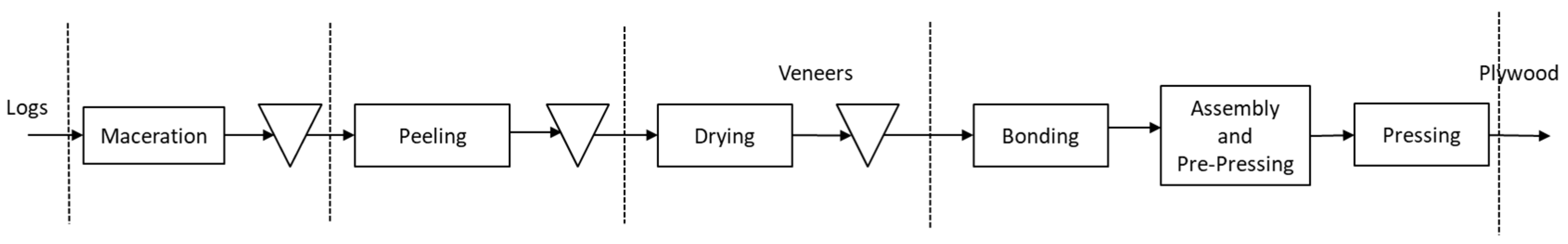
1.1. Description of the Plywood Production Process

Plywood production consists of several key stages—maceration, peeling, drying, bonding, assembly, and pressing—which will be detailed in the next sections (Figure 2 and Figure 3).

1.1.1. Maceration

The production of Pinus radiata plywood begins with debarking freshly harvested logs to ensure a clean surface [9]. The logs are then soaked in water or exposed to steam to soften the wood fibers, reduce hardness, and minimize cracking during peeling or laminating [10]. This process enhances veneer elasticity and surface quality [9,10]. It is carried out in tunnels with a capacity of approximately 180 m³, receiving logs from an irrigation area. Key variables are outlined in

Table 1. Critical factors influencing maceration quality in wood processing [11].

Variable	Impact on Quality
Temperature	Elevated temperatures during the maceration improve wood fiber softening and adhesion, but excessive heat may degrade fibers, weakening structural integrity and visual quality.
Time	Longer maceration enhances fiber softening and adhesion, but excessive durations can lead to fiber breakdown, compromising structure and esthetics.
Intrinsic variable of wood	Uniform, defect-free wood improves maceration results, while defects like knots or cracks increase veneer flaws and reduce structural integrity.

Reproduction with permission from Thays Duarte, Thesis: Use of Machine Learning Techniques to Predict the Quality of Plywood Boards, Professional Qualification, published by Universidad del Bío-Bío, Chile, in 2023.

.

1.1.2. Peeling

The peeling process uses a lathe to rotate logs against a cutting blade, producing continuous veneers of specified dimensions [9]. These veneers are cut, inspected, and trimmed to remove defects such as knots or cracks, ensuring quality. Optimized for softwoods, the process employs stepped transport systems and sensors to enhance material utilization [11,12]. Rotary cutters shape veneers to precise specifications while minimizing flaws. Key variables are shown in

Table 2. Key factors and peeling variables affecting veneer quality, according to [11].

Variable	Impact on Quality
Rotation speed	Ensures uniform cuts and minimizes defects. Excessive speeds cause tear-out; low speeds lead to poor peeling and adhesion.
Knife angle	Optimal angles create clean cuts and uniform thickness. Incorrect angles result in tearing and uneven surfaces.
Feed rate	Consistent feed rates prevent defects. High feed rates cause roughness; low rates lead to overheating and degradation.
Knife position	Proper positioning ensures uniform thickness. Too deep positioning damages fibers; too shallow causes poor peeling.
Density	High-density woods improve strength and cut quality, while low-density woods increase defects and reduce integrity.
Initial temperature	Preheating softens fibers for smoother cuts and better bonding. Low temperatures cause rigidity and defects.

Reproduction with permission from Thays Duarte, Thesis: Use of Machine Learning Techniques to Predict the Quality of Plywood Boards, Professional Qualification, published by Universidad del Bío-Bío, Chile, in 2023.

.

1.1.3. Drying

Freshly cut veneers are dried in rotary dryers or kilns to reduce moisture content, ensuring proper bonding during lamination and preventing defects like warping or cracking from over-drying [13]. This process improves adhesive compatibility and ensures strength and dimensional stability, with an optimal moisture content below 7% [9,13,14]. Drying is energy-intensive, accounting for 70% of thermal energy and 60% of total energy in plywood production [6]. Key variables are outlined in

Table 3. Influence of drying parameters on plywood quality, according to [11,15,16].

Variable	Impact on Quality
Temperature	Optimal drying temperatures remove moisture effectively, preventing defects like warping and splitting. Excessive heat causes fiber degradation, while low temperatures may leave residual moisture.
Initial humidity	High moisture levels cause uneven drying, while low moisture content leads to rapid drying, damaging fibers and weakening adhesion. Optimal moisture content ensures uniform drying and reduces defects.
Vent layout	Proper veneer arrangement ensures uniform airflow and heat distribution, reducing defects. Improper layout causes uneven drying, leading to compromised structural integrity and visual quality.
Feed rate	An optimal feed rate ensures consistent airflow and temperature, preventing defects. Too high a rate leads to insufficient drying, while too slow a rate causes over-drying and fiber degradation.
Air speed	Proper air speed ensures efficient moisture removal and uniform drying, reducing defects. Excessive air speed causes fiber damage, while insufficient air speed leads to uneven drying and structural issues.

.

1.1.4. Bonding

After drying, veneers are coated with adhesives like urea-formaldehyde or phenol-formaldehyde using roller gluing machines for precise dosage control [9]. The veneers, sourced from dry storage in varying sizes (203 cm × 97.6 or 97.6 × 203 cm), are arranged in an interleaved pattern to meet quality and thickness standards [10]. Proper alignment and adhesion during assembly ensure high-quality plywood panels [11]. Key process variables are summarized in

Table 4. Critical parameters for optimizing adhesive performance.

Variable	Impact on Quality
Adhesive flow	Ensures proper penetration into wood fibers, improving mechanical strength. Insufficient flow weakens bonds and risks delamination; excessive flow causes uneven glue distribution and reduced panel strength [9].
Sheet metal temperature	Low temperatures hinder adhesive flow and penetration, weakening bonds. High temperatures cause premature curing, leading to uneven distribution and reduced adhesion strength [10].
Assembly time	Short times prevent proper adhesive wetting, weakening bonds, while long times cause premature drying, reducing effectiveness. Optimal timing ensures strong bonds and structural integrity [9].
Open timeout	Short open times limit adhesive spread, while long times cause premature drying, weakening bonds. Proper timing ensures effective adhesion [11].
Relative humidity	High humidity weakens bonds and risks delamination, while low humidity causes rapid adhesive drying, reducing fiber penetration. Optimal control improves durability [10].
Room temperature	Low temperatures hinder curing, weakening bonds, while high temperatures accelerate curing, reducing working time and causing uneven distribution. Optimal temperature ensures quality adhesion [11].

.

1.1.5. Assembly, Pre-Pressing and Pressing

After adhesive application, veneers are arranged in a “lay-up” sequence, alternating grain direction to enhance strength and stability [17]. The arrangement undergoes pre-pressing, where cold pressure consolidates the layers, ensuring uniform adhesive distribution for the main pressing stage [11]. Pressing is critical for final bonding, with temperature, pressure, and time as key variables. Typical conditions include high pressure (~12.5 bar) and temperature (~138 °C), optimizing the adhesive setting. Curing, traditionally at 100 °C for 2 min, is now conducted often at 120 °C for 7 min to improve efficiency [9,10,11]. Key process variables are detailed in

Table 5. Assembly, pre-pressing and pressing variables.

Variable	Impact on Quality
Pre-pressing time	Adequate pre-pressing time ensures even adhesive distribution. Too little or too much time can weaken bonds [9].
Open wait time	A short open wait time prevents tack development, while long wait causes premature drying, increasing delamination risk [10].
Closed wait time	A short-closed wait time leads to uneven adhesive distribution; long wait causes premature setting, reducing effectiveness [9].
Press cycle time	Insufficient press time can result in incomplete adhesive curing, leading to weak bonds. Excessive press time can cause over-compression, reducing panel thickness and affecting mechanical properties [11].
Press cycle by pressure	Adequate pressure ensures proper adhesive flow and bonding between layers. Insufficient pressure may lead to weak adhesion, while excessive pressure can damage the veneers, compromising structural integrity [10].
Dish position	Proper dish positioning ensures even pressure distribution across the assembly. Misalignment can lead to uneven pressure application, resulting in defects such as warping, delamination, or reduced structural integrity [10].
Plate temperature	Optimal temperature activates adhesive. Low temperatures hinder viscosity; high temperatures degrade adhesive [11].
Pressing pressure	Adequate pressure ensures uniform contact and optimal adhesive distribution; excessive pressure damages veneers [11].
Actual thickness of board in press	Proper thickness ensures even pressure distribution for optimal adhesion. If the board is too thick, it may not receive enough pressure, causing weak bonding. If too thin, excessive pressure can damage veneers or result in uneven adhesive curing [10].
Nominal thickness	Maintaining the specified nominal thickness ensures uniform pressure distribution during pressing, while variations can lead to weak joints and uneven adhesive curing, affecting visual quality [11].
Post-pressing thickness	Post-pressing thickness must meet specified standards to ensure dimensional stability. Inadequate thickness can lead to warping or weak joints, compromising durability and bond strength [11].

.

1.1.6. Quality in Veneer and Plywood

Veneer quality is assessed using key performance indicators (KPIs) like moisture content and visual quality. Moisture content, typically between 8 and 12%, is critical for effective adhesive bonding and durability [18]. Visual quality, which includes color uniformity, grain pattern, and defects such as knots or discoloration, impacts marketability [19]. It is a primary KPI in plywood evaluation, covering surface defects, knot size, and grain alignment, all of which influence esthetics and structural integrity [20]. Ongoing monitoring is essential for maintaining product quality and industry compliance.

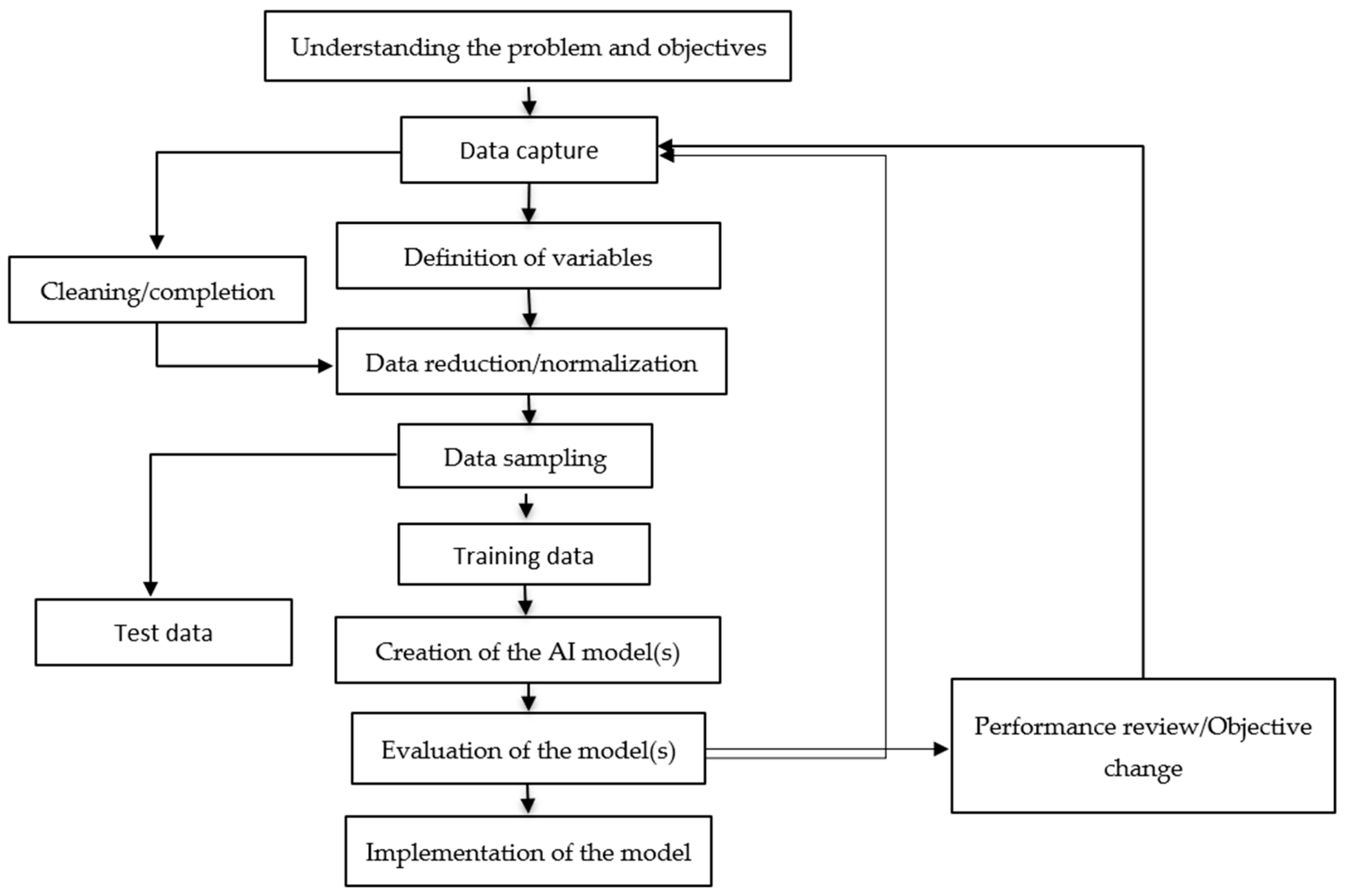
1.2. Machine Learning Approach

ML techniques, a subset of AI, enable capture, deployment, and intelligent analysis of data through sensors in various applications, such as predictive maintenance of industrial plants [21]. ML is utilized for the discovery of “hidden” knowledge from large volumes of data, whether in the form of patterns, correlations, or anomalies, and it has the capability to learn and adapt to new situations [4]. In an ML approach, the quality of the outcome depends, among other factors, on the number of training examples and is restricted by the type and behavior of the parameters or the interaction between response and control factors [3]. Moreover, the ML approach offers greater precision in predicting future actions and allows systems to learn from historical data, including both positive experiences and false positives (erroneous conclusions) [21]. This approach involves modeling the generic behavior of physical processes based on examples, thereby automatically concluding for other situations. In Machine Learning, the choice of algorithm is highly dependent on the nature of the problem, making multiple evaluations necessary. Figure 4 illustrates the general framework for data processing using ML.

ML approaches can be classified into two main categories: unsupervised learning [22] and supervised learning [23]. Unsupervised learning methods are employed to uncover hidden structures within datasets, utilizing set analysis or clustering techniques to reveal subgroups of subjects or objects based on their similarities [24]. By recognizing and identifying these subgroups, data can be organized to achieve a better understanding, improve efficiency, or both [25]. Supervised learning is a fundamental approach in ML, where a model learns from a labeled dataset, where each training example is paired with an output label [26]. The process involves feeding the algorithm with input–output pairs, allowing it to iteratively adjust its internal parameters to minimize the difference between its predicted outputs and the actual labels. This method proves especially effective when the connections between inputs and outputs are clearly established, and the data are abundant and accurately labeled [27]. Among the supervised learning algorithms are the following:

1.3. Least Absolute Shrinkage and Selection Operator (LASSO)

LASSO is a robust regression analysis technique that simultaneously performs variable selection and regularization to enhance both the predictive accuracy and interpretability of the resulting statistical model [28]. By incorporating a penalty equal to the absolute values of the coefficients, LASSO effectively reduces some coefficients to exactly zero. This process simplifies the model by retaining only the most significant predictors [29]. Through this shrinkage, LASSO automatically identifies the most important features, which is particularly advantageous for datasets with many predictors. The inherent feature selection capability of LASSO facilitates clearer model interpretation by establishing a more direct relationship between input variables and predicted outcomes [30]. Additionally, LASSO effectively addresses multicollinearity among predictor variables by selecting one variable from a set of correlated variables while shrinking the others to zero. Consequently, LASSO models tend to generalize better to new data, as the regularization technique mitigates the risk of overfitting, especially in high-dimensional datasets [31]. The key mathematical feature of LASSO is its ability to shrink coefficients and perform variable selection simultaneously by applying an L1 regularization term to the loss function [32]. The LASSO optimization problem can be expressed as Formula (1):

$$\underset{\beta }{\min }\left({\displaystyle \frac{1}{2n}}\sum _{i=1}^n{\left(y_i-X_i^T\beta \right)}^2+\lambda \sum _{j=1}^p\left|{\beta }_j\right|\right)$$

(1)

where $y_i$ represents the response variable, $X_i$ and β are the predictors, λ is the regularization parameter, and p is the number of predictors. The L1 penalty $\sum _{j=1}^p\left|{\beta }_j\right|$ forces some of the coefficients β_j to be exactly zero when λ is large enough, leading to sparse solutions.

1.4. K-Nearest Neighbors (kNN)

It is a non-parametric, instance-based learning approach that functions by locating the ‘k’ nearest neighbors in the feature space and determining the output based on majority voting for classification or averaging for regression [33]. An advantage of kNN is its ease of implementation and ability to handle multi-class classification without requiring prior assumptions. Common applications include pattern recognition, recommendation systems, and image classification [34].

1.5. Support Vector Machines (SVMs)

It is an effective supervised learning algorithm that determines the optimal hyperplane to maximize separation of data points into distinct classes [35]. In cases when data cannot be separated linearly, SVM applies kernel functions to map into higher-dimensional spaces, enabling more complex decision boundaries [36]. A key advantage of SVM is its effectiveness in managing high-dimensional data efficiently and its resilience to overfitting, particularly when working with small datasets [37].

1.6. Random Forest

Random Forest operates by generating an ensemble of decision trees during training, where each tree represents a random subset of features and samples. The ultimate prediction made by aggregating the results of these individual trees, either through voting (for classification) or averaging (for regression) [38]. This method reduces overfitting and improves generalization due to the diversity among the trees. Key advantages of Random Forest include its ability to handle large datasets with high dimensionality, its robustness against noise, and its effectiveness in managing missing data [39]. Additionally, Random Forest provides an internal measure of feature importance, which is valuable for feature selection [40].

1.7. XGBoost

This is a powerful and adaptable approach to gradient-boosted decision trees designed and optimized for computational efficiency [41]. XGBoost implements the gradient boosting framework by sequentially building a series of decision trees, where each new tree aims to reduce the errors of the previous trees. XGBoost can handle missing values by learning the best direction when a value is missing, which is especially useful in real-world datasets where missing values are common. XGBoost allows for custom objective functions, making it highly flexible for various tasks beyond classification and regression, such as ranking and user-defined metrics [42].

1.8. Logistic Regression

It is a commonly applied statistical approach for handling binary classification tasks, in which the outcome is categorical, typically coded as 0 or 1 [43]. Unlike linear regression, which models a continuous output, Logistic Regression predicts the probability of a binary response using the logistic function. The function maps predicted values to probabilities between 0 and 1, making it ideal for classification tasks. Its advantages include simplicity and interpretability, offering a detailed understanding of the connections between predictor variables and the outcome. Additionally, it is computationally efficient and performs well on small to moderately sized datasets [44].

1.9. Machine Learning in Plywood Industry

The application of AI and ML tools in the plywood panel manufacturing industry remains in its nascent stages. Urra and Ramos [45] utilized ML to predict adhesion under industrial operating conditions during the gluing and pre-pressing stages of wooden boards. They optimized cutting patterns for Pinus radiata D. Don trunks with defective cylindrical cores using 3D technology. Gradov et al. [6] developed a continuous drying model for wood veneers based on mass and energy balances to maximize process efficiency, optimizing energy requirements through an ANOVA analysis. Lastly, Demir [46] employed Artificial Neural Networks (ANNs) to assess the impact of urea-formaldehyde resin filler on the bond strength of plywood panels. Finally, in a recently published study, Ramos et al. [8] evaluated the performance of various ML algorithms for predicting the quality of the veneer drying process, concluding that eXtreme Gradient Boosting achieved an accuracy of 76% in forecasting quality outcomes.

In this study, supervised algorithms were employed to predict the quality of industrially processed Pinus radiata veneers.

The novelty of this article lies in the use of large-scale online industrial data combined with AI to predict veneer quality. To date, no research has been conducted on predicting quality in the panel and plywood manufacturing process. Leveraging industrial data and exploring the application of AI algorithms—particularly ML—to forecast key performance indicators (KPIs) in process plants represents an innovative approach.

2. Resources and Data Processing

2.1. Computational and ML Resources

An Asus computer equipped with an Intel Core i9-13900 KF processor with 32 cores, a processing speed of 3.0 GHz, and 65 GB of RAM was utilized. Python (Version 3.12.6) (2024) was employed for developing the algorithms used in data analysis [47]. The libraries employed were Numpy (version 1.24.0), Scikit-Learn (version 1.1.3), Pandas (version 1.5.3), and Matplotlib (version 3.6.3). The programming functions were train_test_split, cross_val_score, MinMaxScaler, classification_report, confusion_matrix, ConfusionMatrixDisplay, accuracy_score, precision_score, recall_score, f1_score, and LabelEncoder.

Models were tuned with GridSearchCV of Scikit-Learn Library. GridSearchCV optimizes a model’s hyperparameters using cross-validation, and it helps find the best combination of parameters without manual testing.

Data Model, Data Flow and Collection

The data were obtained from an industrial process for manufacturing Pinus radiata plywood. The plant produces approximately 350,000 m³ of plywood annually. The species (Pinus radiata) sourced from the central–southern region of Chile [48]. The data from the OPC server were collected and stored in a PI System© (from AVEVA, Cambridge, UK) server using the PI DataLink Excel add-in. Data captured from various sensors were transmitted via PI System© to a SQL database. The methodology follows the classical steps of the ML framework (Figure 5).

2.2. Collected Variables

The industrial data of Pinus radiata veneers originate from three subprocesses: maceration, peeling, and drying. It is important to emphasize that the measurement of the variables listed in

Table 6. Variables effectively measured to assess the quality of Pinus radiata veneers.

Variable	Abbreviation	Units	Subprocess
Maceration temperature	MT	°C	Maceration
Maceration time	Mt	h	Maceration
Rotation speed	Rs1 and Rs2	rpm	Peeling
Knife angle	Ka1 and Ka2	°	Peeling
Feed rate	Fr1 and Fr2	m/min	Peeling
Mantle temperature	MT1 and MT2	°C	Peeling
Horizontal opening of the lathe	Ho1 and Ho2	mm	Peeling
Linear meters veneer produced	Lm1 and Lm2	m	Peeling
Log diameter	Lg1 and Lg2	cm	Peeling
Nominal thickness of veneer	Nt1 and Nt2	mm	Peeling
Drying temperature	DT151, DT152, DT153, DT181, DT182, DT183, DT241, DT242 and DT243	°C	Drying
Moisture veneer	MV151, MV152, MV153, MV181, MV182, MV183, MV241, MV242 and MV243	%	Drying
Vapor pressure	VP151, VP152, VP153, VP181, VP182, VP183, VP241, VP242 and VP243	bar	Drying
Dryer speed	Ds24	m/s	Drying
Steam inlet temperature	SiT24	°C	Drying
Steam inlet pressure	Sip24	°C	Drying
Vent opening	VO24	%	Drying

is conducted in-line. The industrial data are collected through sensors conveniently installed in each subprocess. The variables measured in this process are presented below.

A part of the database is shown in

Table 7. Example of dataset (some variables).

TS	Maceration Time, h	Maceration Temperature °C	Rotation Speed Rs1, rpm	Knife Angle Ka1, °	Feed Rate Fr1	Mantle TemperatureMT1, °C	Horizontal Opening of the Lathe Ho1, mm	Log Diameter Lg1 cm	Nominal Thickness Nt1, mm
2024-04-09 17:10:00	17.9	79.2	320	0.39	250	49	−0.45	51.8	2.55
2024-04-09 17:15:00	17.9	78.9	320	−0.5	250	49	−0.45	51.8	2.55
2024-04-09 17:20:00	17.9	78.8	320	−0.49	250	47	−0.45	55.2	2.55

. Each data line corresponds to a single record.

Each row is collected at one specific time stamp (TS). Rows are identified by a quality index of the veneer like 1: “high quality” or 0: “low quality”. The complete collected data of 13,690 records are converted to a dataset. Table 7 presents an extract.

2.3. Data Preprocessing

First, data cleaning was carried out to remove outliers and missing values. Empty (null) cells were filled with the values of the previous existing cells. The objective was to replace null values with the nearest valid values of the same variable.

Subsequently, data normalization was applied to ensure uniform scaling and weighting throughout the analysis. Normalization was applied on the whole dataset. The normalization process was carried out using Equation (2) [8]:

$$X_{norm}={\displaystyle \frac{X-X_{min}}{X_{max}-X_{min}}}$$

(2)

where X_norm is the data normalized between 0 and 1, X is the data to be normalized, X_min is the minimum value of the data, and X_max is the maximum value of the data.

The dataset, which includes maceration, peeling, and drying variables, originally contained 49 variables. To reduce dimensionality, a correlation matrix was employed. Correlation analysis is a fundamental statistical tool used to assess the relationship between two quantitative variables. It plays a crucial role in identifying and quantifying the strength and direction of associations between variables [49].

Correlation measures the extent and direction of a linear relationship between two variables. A positive correlation indicates that as one variable increases, the other tends to increase as well. Conversely, a negative correlation suggests that as one variable increases, the other tends to decrease. If no correlation is present, the variables do not exhibit a clear linear trend [26].

The Pearson correlation coefficient (r) is the most widely used metric for quantifying the linear correlation between two variables. It is calculated using Equation (3) [49]:

$$r={\displaystyle \frac{{\sum }_{i=1}^n\left(x_i-\dot{x}\right)-\left(y_i-\dot{y}\right)}{\sqrt{{\sum }_{i=1}^n{\left(x_i-\dot{x}\right)}^2{\sum }_{i=1}^n{\left(y_i-\dot{y}\right)}^2}}}$$

(3)

where x_i and y_i are the individual values of the variables x and y, respectively, and ẋ and ẏ are the means of x and y.

The coefficient r takes values between −1 and 1. A value of r=1 indicates a perfect positive correlation, r = −1 a perfect negative correlation, and r = 0 suggests no linear correlation. The magnitude of the correlation coefficient indicates the strength of the relationship between variables. Values close to 1 or −1 indicate strong relationships, while values close to 0 indicate weak or nonexistent relationships. It is important to note that r only measures linear relationships and does not imply causality between variables.

The variable reduction process was applied to a dataset constructed from data collected online at one-second intervals over a two-month operational period of the plant. Correlation analysis was performed on the 49 available variables from the three analyzed processes: maceration, peeling, and drying. Subsequently, for training and testing ML algorithms, a new dataset was created using data collected at five-minute intervals. A correlation threshold of 0.85 was established as the selection criterion. It was verified that reducing variables up to this correlation value (0.85) does not impact process variability in terms of key performance indicators (accuracy, precision, and recall). After applying the correlation matrix, the Least Absolute Shrinkage and Selection Operator (LASSO) algorithm was utilized to further refine the variable selection process.

The dataset, which includes maceration, peeling, and drying variables, originally comprised 49 variables (Table 6). Data were collected at 10-minute intervals, ensuring real-time synchronization for all 49 variables across the subprocesses (maceration, peeling, and drying). Subsequently, veneer quality labels—moisture content and visual quality—were incorporated into the dataset. The data were then split into two categories: training data (70%) and validation and test data (30%) [12].

The following supervised algorithms are used to obtain the metrics: kNN, SVM, RF, XGBoost and Logistic Regression.

To assess the performance of the models, a confusion matrix was used [50], which compares the model’s predictions with the actual class label values: true positive (TP): cases where the model correctly predicts the positive class; true negative (TN): cases where the model correctly predicts the negative class; false positive (FP): cases where the model incorrectly predicts the positive class, when the actual value is negative (Type I error); and false negative (FN): cases where the model incorrectly predicts the negative class, when the actual value is positive (Type II error) [51] (Figure 6).

Once the values in Figure 6 were obtained, the evaluation metrics were calculated [53]. Accuracy, defined as the proportion of correctly classified predictions by the model, was determined (Equation (4)). Additionally, precision, which measures how close the predicted values are to the true values, was calculated (Equation (5)). Recall, representing the true positive rate or the proportion of correctly classified positive cases relative to the total number of positives, was also evaluated (Equation (6)).

Finally, the F1-score (Equation (7)) was computed as a performance metric for the classification model, particularly in cases of imbalanced datasets. The F1-score is the harmonic mean of precision and recall, providing a single measure that balances both metrics. This metric is particularly useful when there is an uneven class distribution, as it accounts equally for false positives and false negatives. A high F1-score indicates that the model achieves both high precision and high recall, offering a more balanced measure of performance compared to using either precision or recall alone [54,55].

$$Accuracy={\displaystyle \frac{TP+TN}{TP+TN+FP+FN}}$$

(4)

$$Precision={\displaystyle \frac{TP}{TP+FN}}$$

(5)

$$Recall={\displaystyle \frac{TP}{TP+FP}}$$

(6)

$$Accuracy={\displaystyle \frac{TP+TN}{TP+TN+FP+FN}}$$

(7)

2.4. Experimental Design

For the evaluation of the process up to obtaining sheets, 13,690 records were collected. The experimental design for supervised algorithms considers the following:

• Data Collection Interval: (1) every 5 min;
• Data Split: 70% training data, 30% test data;
• Algorithms Used: Random Forest, XGBoost, K-Nearest Neighbors (KNN), Support Vector Machine (SVM), Lasso, and Logistic Regression;
• KPI: Sheet Quality;
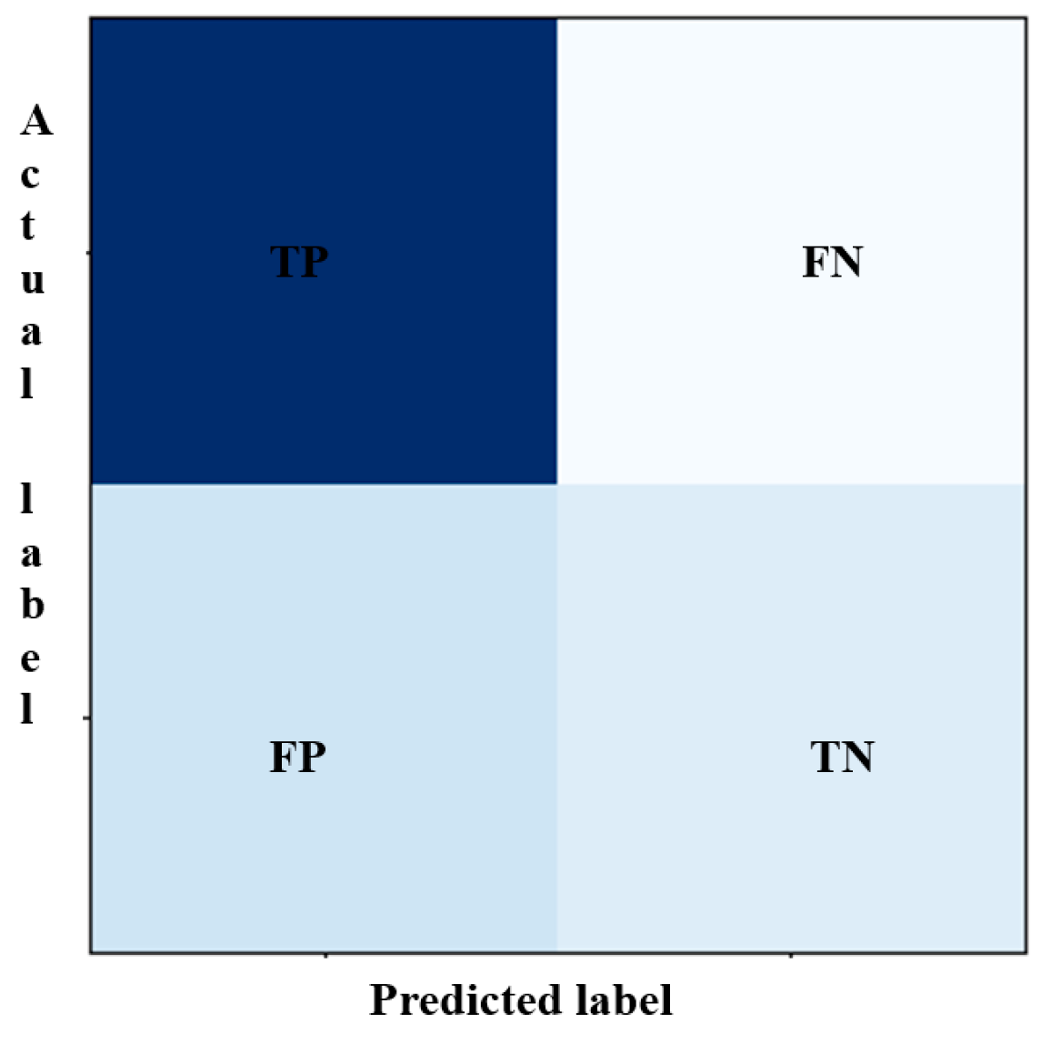
• Performance Metrics: Accuracy, Precision, Recall, F1-score.

3. Results and Discussion

3.1. Data Reduction

The correlation matrix (Supplementary Figure S1) was used to identify variable relationships greater than 0.85, allowing the reduction in the initial 49 variables. From the initial 49 variables, 12 were reduced, all originating from the drying process. This is consistent, as three measurements were taken for each dryer (at the inlet, in the middle, and at the outlet). The variables from the middle of the dryer were retained in the analysis, as this is where most of the moisture from the veneer is effectively removed. Therefore, variables with high correlation at the inlet and outlet of the dryer were eliminated. After applying the correlation matrix, the following 12 variables were eliminated: DT151, DT153, DT181, DT183, DT241, DT243, VP151, VP153, VP181, VP183, MV153 and MV183.

3.2. LASSO

The LASSO algorithm is widely utilized for variable reduction in datasets due to its ability to enhance model interpretability and prevent overfitting [29]. By imposing an L1 penalty on the coefficients, LASSO effectively drives some coefficients to zero, thereby selecting only the most significant predictors.

A comprehensible pseudocode is shown as Algorithm 1 [29]:

Algorithm 1. LASSO Regression

Input:    - X: Feature matrix (n x p) where n is the number of samples and p is the number of features  - y: Target variable (n x 1)  - λ (lambda): Regularization parameter controlling sparsity  - Max_iterations: Maximum number of optimization steps  - Tolerance: Convergence threshold  Output:   - β: Estimated coefficient vector (p x 1)  Steps:  1. Initialize β (coefficients) to zeros or small random values.  2. Standardize the feature matrix X (zero mean and unit variance for each feature).  3. Repeat until convergence or Max_iterations is reached:    a. For each feature j in X:      i. Compute the partial residual:        r_j = y − (X * β) + (X_j * β_j)      ii. Compute the ordinary least squares estimate:        β_j = (1/n) * Σ (X_j * r_j)      iii. Apply the soft-thresholding function:        β_j = sign(β_j) * max(|β_j| − λ, 0)    b. Check for convergence:        - If the maximum absolute change in β between iterations is smaller than Tolerance, stop.  4. Return the final β values.  End Algorithm

This feature selection capability is particularly beneficial in high-dimensional datasets, where multicollinearity may obscure the relationships between variables. Consequently, LASSO not only simplifies models but also improves predictive accuracy, making it a valuable tool in statistical modeling and ML. After applying the LASSO algorithm, the following six variables were eliminated: Mt, FR1, Nt2, MV181, MV243 and SiT24.

3.3. Data Processing

The confusion matrix (

Table 8. Confusion matrix.

Algorithm	Actual Label	Predicted Label
		0	1
kNN	0	2493	362
	1	647	605
SVM	0	2791	64
	1	993	259
RF	0	2601	254
	1	724	528
XGB	0	2558	297
	1	702	550
Logic	0	2734	121
	1	975	277
LASSO	0	2757	98
	1	1.009	243

) is a valuable tool for evaluating the performance of classification algorithms, providing insights into accuracy, precision, recall, and F1-score metrics. In this study, several algorithms were assessed, including K-Nearest Neighbors (KNN), Support Vector Machine (SVM), Random Forest (RF), XGBoost (XGB), Logistic Regression, and LASSO.

The results indicate that the Random Forest algorithm achieved the highest accuracy of 0.76, followed closely by XGBoost. KNN exhibited a notable precision of 0.63, while SVM demonstrated a precision of 0.80, albeit with a lower recall of 0.21. LASSO and Logistic Regression showed lower performance across metrics, with accuracies of 0.73 and similar precision and recall values. These findings underscore the varying strengths of each algorithm, highlighting the importance of selecting appropriate models based on the specific characteristics of the dataset.

3.4. Metrics

The following results, presented in

Table 9. Metrics.

Algorithm	Accuracy	Precision	Recall	F1-Score
KNN	0.75	0.63	0.48	0.55
SVM	0.74	0.80	0.21	0.33
RF	0.76	0.68	0.42	0.52
XGB	0.76	0.65	0.44	0.52
Logic	0.73	0.22	0.34	0.34
Lasso	0.73	0.19	0.31	0.31

, are derived from the evaluation of various classification algorithms using the confusion matrix. Key performance metrics, including accuracy, precision, recall, and F1-score, are provided to highlight the effectiveness of each algorithm, offering insights into model performance for optimal algorithm selection. The results indicate that the Random Forest algorithm achieved the highest accuracy of 0.76, followed closely by XGBoost. KNN exhibited a precision of 0.63, while SVM demonstrated a precision of 0.80, albeit with a lower recall of 0.21. LASSO and Logistic Regression showed lower performance across metrics, with accuracies of 0.73 and similar precision and recall values. These findings underscore the varying strengths of each algorithm. Emphasizing the necessity of choosing suitable models according to the dataset’s specific characteristics.

4. Conclusions

In the collected data, the challenge of establishing connections between the industrial data source and the data processing center was successfully addressed. A dataset containing 13,690 records was compiled, with periodic entries collected every 5 min.

Industrial data and ML were successfully applied to a prediction model to assess veneer quality in plywood manufacturing. This approach involved analyzing the maceration, peeling, and drying processes, utilizing a dataset with 49 original variables. After removing correlated variables, the dataset was reduced to 37 variables. Finally, following LASSO-based feature selection, each algorithm used 30 variables. The dataset contained a total of 13,690 records, with 9520 labeled as low in quality and 4170 as high in quality.

This study highlights the varying performance of classification algorithms by analyzing accuracy, precision, recall, and F1-score metrics, as detailed in the confusion matrix. Among the models evaluated, Random Forest demonstrated the highest effectiveness, achieving an accuracy of 0.76, making it particularly suitable for applications where overall correctness is critical. XGBoost also performed well, positioning itself as a strong alternative for scenarios requiring a balance between accuracy and recall. SVM, with its high precision (0.80) but lower recall (0.21), may be preferable in cases where precision is more important than recall. Meanwhile, K-Nearest Neighbors (KNN) achieved respectable precision but did not surpass Random Forest or XGBoost in accuracy. LASSO and Logistic Regression showed moderate effectiveness, suggesting that these models may be less suitable for datasets with high complexity or nuanced class boundaries.

This comparison underscores the importance of selecting algorithms based on dataset characteristics, providing a framework for optimizing model selection in future applications.

The main limitation of this study was the availability of a larger dataset. The 13,000 records collected at 10 min intervals represent approximately 90 days of continuous 24/7 operation. A longer data collection period is necessary to ensure greater robustness and improve the performance of the algorithms. Additionally, extending the timeframe would capture a wider range of working conditions, allowing the models to learn from a broader spectrum of operational scenarios.

Future research should explore unsupervised learning techniques to identify patterns in plant operations, such as through clustering algorithms. This could lead to the discovery of process operation modes and varying quality levels. While this study considered only two quality categories, in industrial practice, quality assessment is often more nuanced. Pattern detection could be enhanced using deep learning algorithms.

Finally, modeling the entire plant process up to the final product remains an ongoing research focus for our team.

References

1. Ramos-Maldonado, M.; Aguilera-Carrasco, C. Trends and Opportunities of Industry 4.0 in Wood Manufacturing Processes; Intechopen: London, UK, 2021. [Google Scholar] [CrossRef]
2. Orejuela-Escobar, L.; Venegas-Vásconez, D.; Méndez, M.A. Opportunities of Artificial Intelligence in Valorisation of Biodiversity, Biomass and Bioresidues—Towards Advanced Bio-Economy, Circular Engineering, and Sustainability. Int. J. Sustain. Energy Environ. Res. 2024, 13, 105–113. [Google Scholar] [CrossRef]
3. Lu, Z.; Lin, F.; Ying, H. Design of Decision Tree via Kernelized Hierarchical Clustering for Multiclass Support Vector Machines. Cybern. Syst. 2007, 38, 187–202. [Google Scholar] [CrossRef]
4. Shalev-Shwartz, S.; Ben-David, S. Understanding Machine Learning: From Theory to Algorithms; Cambridge University Press: Cambridge, UK, 2014; ISBN 978-1-107-05713-5. [Google Scholar]
5. Frey, U.J.; Klein, M.; Deissenroth, M. Modelling Complex Investment Decisions in Germany for Renewables with Different Machine Learning Algorithms. Environ. Model. Softw. 2019, 118, 61–75. [Google Scholar] [CrossRef]
6. Gradov, D.V.; Yusuf, Y.O.; Ohjainen, J.; Suuronen, J.; Eskola, R.; Roininen, L.; Koiranen, T. Modelling of a Continuous Veneer Drying Unit of Industrial Scale and Model-Based ANOVA of the Energy Efficiency. Energy 2022, 244, 122673. [Google Scholar] [CrossRef]
7. Venegas-Vásconez, D.; Orejuela-Escobar, L.; Valarezo-Garcés, A.; Guerrero, V.H.; Tipanluisa-Sarchi, L.; Alejandro-Martín, S. Biomass Valorization through Catalytic Pyrolysis Using Metal-Impregnated Natural Zeolites: From Waste to Resources. Polymers 2024, 16, 1912. [Google Scholar] [CrossRef]
8. Ramos Maldonado, M.; Duarte Sepúlveda, T.; Gatica Neira, F.; Venegas Vásconez, D. Machine Learning Para Predecir La Calidad Del Secado de Chapas En La Industria de Tableros Contrachapados de Pinus Radiata. Maderas Cienc. Tecnol. 2024, 26, 1–18. [Google Scholar] [CrossRef]
9. Teihuel, J. Propuesta de Alternativas de Solución Para El Transporte de residuos de Madera Sólida En La Industria de Tableros. Bachelor’s Thesis, Universidad Austral de Chile, Los Rios Region, Chile, 2007. [Google Scholar]
10. Moisan, R. Modelo de Determinación de Rendimiento Para El Proceso de Elaboración de Paneles En Planta Nueva Aldea. Bachelor’s Thesis, Universidad del Bío-Bío, Concepción City, Chile, 2007. [Google Scholar]
11. Duarte, T. Uso de Técnicas de Machine Learning Para Predecir La Calidad de Tableros Contrachapados. Habilitación Profesional. Bachelor’s Thesis, Universidad del Bío-Bío, Concepción City, Chile, 2023. [Google Scholar]
12. Navarrete, C. Evaluación de Método Predictivo Para Variables de Secado de Chapas En Planta de Paneles Arauco Nueva Aldea. Habilitación Profesional. Bachelor’s Thesis, Universidad del Bío-Bío, Concepción City, Chile, 2020. [Google Scholar]
13. Kehr, R. Evaluación de Programas de Secado Continuo En Chapas de Pinus Radiata D. Don. Bachelor’s Thesis, Universidad Austral de Chile, Los Rios Region, Chile, 2007. [Google Scholar]
14. Aydin, I. Effects of veneer drying at high temperature and chemical treatments on equilibrium moisture content of plywood. Maderas Cienc. Tecnol. 2014, 16, 445–452. [Google Scholar] [CrossRef]
15. Demirkir, C.; Özsahin, Ş.; Aydin, I.; Colakoglu, G. Optimization of Some Panel Manufacturing Parameters for the Best Bonding Strength of Plywood. Int. J. Adhes. Adhes. 2013, 46, 14–20. [Google Scholar] [CrossRef]
16. Lutz, J. Wood and Log Characteristics Affecting Veneer Production. In USDA Forest Service Research Paper; Forest Products Laboratory: Madison, WI, USA, 1971. [Google Scholar]
17. Shi, S.; Walker, J. Wood-based composites: Plywood and veneer-based products. In Primary Wood Processing; Springer: Berlin/Heidelberg, Germany, 2006. [Google Scholar] [CrossRef]
18. Yuan, Y.; Zhang, S.; Li, X. Moisture Content Distribution and Its Effect on Veneer Properties. J. Wood Sci. 2017, 63, 49–55. [Google Scholar]
19. Kollmann, F.F.P.; Côté, W.A. Solid Wood. In Principles of Wood Science and Technology; Springer: Berlin/Heidelberg, Germany, 1984. [Google Scholar]
20. Lai, W.; Zhao, H.; Zhang, Y. Influence of Wood Surface Characteristics on Plywood Quality. Wood Sci. Technol. 2019, 53, 47–64. [Google Scholar]
21. Wu, S.J.; Gebraeel, N.; Lawley, M.A.; Yih, Y. A Neural Network Integrated Decision Support System for Condition-Based Optimal Predictive Maintenance Policy. IEEE Trans. Syst. Man Cybern. Part A Syst. Hum. 2007, 37, 226–236. [Google Scholar] [CrossRef]
22. Minaei-Bidgoli, B.; Parvin, H.; Alinejad-Rokny, H.; Alizadeh, H.; Punch, W.F. Effects of Resampling Method and Adaptation on Clustering Ensemble Efficacy. Artif. Intell. Rev. 2014, 41, 27–48. [Google Scholar] [CrossRef]
23. Parvin, H.; Alinejad-Rokny, H.; Minaei-Bidgoli, B.; Parvin, S. A New Classifier Ensemble Methodology Based on Subspace Learning. J. Exp. Theor. Artif. Intell. 2013, 25, 227–250. [Google Scholar] [CrossRef]
24. Pillay, T.; Cawthra, H.C.; Lombard, A.T. Integration of Machine Learning Using Hydroacoustic Techniques and Sediment Sampling to Refine Substrate Description in the Western Cape, South Africa. Mar. Geol. 2021, 440, 106599. [Google Scholar] [CrossRef]
25. Burghardt, E.; Sewell, D.; Cavanaugh, J. Agglomerative and Divisive Hierarchical Bayesian Clustering. Comput. Stat. Data Anal. 2022, 176, 107566. [Google Scholar] [CrossRef]
26. Lecun, Y.; Bengio, Y.; Hinton, G. Deep Learning. Nature 2015, 521, 436–444. [Google Scholar] [CrossRef]
27. Esteva, A.; Kuprel, B.; Novoa, R.A.; Ko, J.; Swetter, S.M.; Blau, H.M.; Thrun, S. Dermatologist-Level Classification of Skin Cancer with Deep Neural Networks. Nature 2017, 542, 115–118. [Google Scholar] [CrossRef]
28. Coleman, K.D.; Schmidt, K.; Smith, R.C. Frequentist and Bayesian Lasso Techniques for Parameter Selection in Nonlinearly Parameterized Models. IFAC-PapersOnLine 2016, 49, 416–421. [Google Scholar] [CrossRef]
29. Tibshirani, R. Regression Shrinkage and Selection via the Lasso. J. R. Stat. Soc. Ser. B (Methodol.) 1996, 58, 267–288. [Google Scholar] [CrossRef]
30. Lindström, E.; Höök, J. Unbiased Adaptive LASSO Parameter Estimation for Diffusion Processes; Elsevier B.V.: Amsterdam, The Netherlands, 2018; Volume 51, pp. 257–262. [Google Scholar]
31. Zhang, Y.; Haghani, A. A Gradient Boosting Method to Improve Travel Time Prediction. Transp. Res. Part C Emerg. Technol. 2015, 58, 308–324. [Google Scholar] [CrossRef]
32. Zou, H.; Hastie, T. Regularization and Variable Selection via the Elastic Net. J. R. Stat. Soc. Ser. B (Stat. Methodol.) 2005, 67, 301–320. [Google Scholar] [CrossRef]
33. Ali, A.; Hamraz, M.; Khan, D.; Debani, W.; Khan, Z. A Random Projection k Nearest Neighbours Ensemble for Classification via Extended Neighbourhood Rule. arXiv 2023, arXiv:2303.12210. [Google Scholar] [CrossRef]
34. Jodas, D.S.; Passos, L.A.; Adeel, A.; Papa, J.P. PL-KNN: A parameterless nearest neighbors classifier. In Proceedings of the 2022 29th International Conference on Systems, Signals and Image Processing (IWSSIP), Sofia, Bulgaria, 1–3 June 2022. [Google Scholar] [CrossRef]
35. Liu, Z.; Kou, J.; Yan, Z.; Wang, P.; Liu, C.; Sun, C.; Shao, A.; Klein, B. Enhancing XRF Sensor-Based Sorting of Porphyritic Copper Ore Using Particle Swarm Optimization-Support Vector Machine (PSO-SVM) Algorithm. Int. J. Min. Sci. Technol. 2024, 34, 545–556. [Google Scholar] [CrossRef]
36. Onyelowe, K.C.; Mahesh, C.B.; Srikanth, B.; Nwa-David, C.; Obimba-Wogu, J.; Shakeri, J. Support Vector Machine (SVM) Prediction of Coefficients of Curvature and Uniformity of Hybrid Cement Modified Unsaturated Soil with NQF Inclusion. Clean Eng. Technol. 2021, 5, 100290. [Google Scholar] [CrossRef]
37. Zheng, M.; Luo, X. Joint Estimation of State of Charge (SOC) and State of Health (SOH) for Lithium Ion Batteries Using Support Vector Machine (SVM), Convolutional Neural Network (CNN) and Long Sort Term Memory Network (LSTM) Models. Int. J. Electrochem. Sci. 2024, 19, 100747. [Google Scholar] [CrossRef]
38. Breiman, L. Random Forests. Mach. Learn. 2001, 45, 5–32. [Google Scholar] [CrossRef]
39. Díaz-Uriarte, R.; Alvarez de Andrés, S. Gene Selection and Classification of Microarray Data Using Random Forest. BMC Bioinform. 2006, 7, 3. [Google Scholar] [CrossRef]
40. Cutler, D.R.; Edwards, T.C.; Beard, K.H.; Cutler, A.; Hess, K.T.; Gibson, J.; Lawler, J.J. Random Forests for Classification in Ecology. Ecology 2007, 88, 2783–2792. [Google Scholar] [CrossRef]
41. Wang, Q.; Zou, X.; Chen, Y.; Zhu, Z.; Yan, C.; Shan, P.; Wang, S.; Fu, Y. XGBoost Algorithm Assisted Multi-Component Quantitative Analysis with Raman Spectroscopy. Spectrochim. Acta Part A Mol. Biomol. Spectrosc. 2024, 323, 124917. [Google Scholar] [CrossRef]
42. Wang, Z.H.; Liu, Y.F.; Wang, T.; Wang, J.G.; Liu, Y.M.; Huang, Q.X. Intelligent Prediction Model of Mechanical Properties of Ultrathin Niobium Strips Based on XGBoost Ensemble Learning Algorithm. Comput Mater Sci 2024, 231, 112579. [Google Scholar] [CrossRef]
43. Hosmer, D.W., Jr.; Lemeshow, S.; Sturdivant, R.X. Applied Logistic Regression; John WiIley: Hoboken, NJ, USA, 2000. [Google Scholar]
44. Joanne Peng, C.-Y.; Lee, K.L.; Ingersoll, G. An Introduction to Logistic Regression Analysis and Reporting. J. Educ. Res. 2002, 96, 3–14. [Google Scholar] [CrossRef]
45. Urra-González, C.; Ramos-Maldonado, M. A Machine Learning Approach for Plywood Quality Prediction. Maderas Cienc. Tecnol. 2023, 25, 36. [Google Scholar] [CrossRef]
46. Demir, A. Determination of the Effect of Valonia Tannin When Used as a Filler on the Formaldehyde Emission and Adhesion Properties of Plywood with Artificial Neural Network Analysis. Int. J. Adhes. Adhes. 2023, 123, 103346. [Google Scholar] [CrossRef]
47. Manrique Rojas, E. Machine Learning: Análisis de Lenguajes de Programación y Herramientas Para Desarrollo. Rev. Ibérica Sist. Tecnol. Informação 2019, 28, 586–599. [Google Scholar]
48. Venegas-Vásconez, D.; Arteaga-Pérez, L.E.; Aguayo, M.G.; Romero-Carrillo, R.; Guerrero, V.H.; Tipanluisa-Sarchi, L.; Alejandro-Martín, S. Analytical Pyrolysis of Pinus Radiata and Eucalyptus Globulus: Effects of Microwave Pretreatment on Pyrolytic Vapours Composition. Polymers 2023, 15, 3790. [Google Scholar] [CrossRef]
49. Russell, S.J.; Norvig, P. Artificial Intelligence: A Modern Approach, 4th ed.; Pearson Educational Inc.: London, UK, 2021; ISBN 9780134610993. [Google Scholar]
50. Luque, A.; Carrasco, A.; Martín, A.; de las Heras, A. The Impact of Class Imbalance in Classification Performance Metrics Based on the Binary Confusion Matrix. Pattern Recognit. 2019, 91, 216–231. [Google Scholar] [CrossRef]
51. Nakamura, K. A Practical Approach for Discriminating Tectonic Settings of Basaltic Rocks Using Machine Learning. Appl. Comput. Geosci. 2023, 19, 100132. [Google Scholar] [CrossRef]
52. Düntsch, I.; Gediga, G. Confusion Matrices and Rough Set Data Analysis. J. Phys. Conf. Ser. 2019, 1229, 012055. [Google Scholar] [CrossRef]
53. Lu, G.; Zeng, L.; Dong, S.; Huang, L.; Liu, G.; Ostadhassan, M.; He, W.; Du, X.; Bao, C. Lithology Identification Using Graph Neural Network in Continental Shale Oil Reservoirs: A Case Study in Mahu Sag, Junggar Basin, Western China. Mar. Pet. Geol. 2023, 150, 106168. [Google Scholar] [CrossRef]
54. Bressan, T.S.; Kehl de Souza, M.; Pirelli, T.J.; Junior, F.C. Evaluation of Machine Learning Methods for Lithology Classification Using Geophysical Data. Comput. Geosci. 2020, 139, 104475. [Google Scholar] [CrossRef]
55. Lundberg, S.M.; Allen, P.G.; Lee, S.-I. A Unified Approach to Interpreting Model Predictions. In Proceedings of the Conference on Neural Information Processing Systems (NIPS), Long Beach, CA, USA, 4–9 December 2017. [Google Scholar] [CrossRef]
Figure 1. Plywood panels (https://mx.arauco.com/c/products/ct-triplay/br-arply, accessed on 1 March 2025).
Processes 13 01229 g001
Figure 2. Plywood process.
Processes 13 01229 g002
Figure 3. An industrial drying and transfer line (www.raute.com/lines-and-machines/lines/veneer-drying/veneer-drying-line-r7/, accessed on 1 March 2025).
Processes 13 01229 g003
Figure 4. IA and data approach framework.
Processes 13 01229 g004
Figure 5. Data model and data flow diagram for industrial data collection.
Processes 13 01229 g005
Figure 6. Confusion matrix for binary classification. Adapted from [52].
Processes 13 01229 g006