Theory-Driven Multi-Output Prognostics for Complex Systems Using Sparse Bayesian Learning

Abstract

Complex systems often face significant challenges in both efficiency and performance when making long-term degradation predictions. To address these issues, this paper proposes a predictive architecture based on multi-output sparse probabilistic model regression. An adaptive health index (HI) extraction method was also introduced, which leverages unsupervised deep learning and variational mode decomposition to effectively extract health indicators from multiple measurements of complex systems. The effectiveness of the proposed method was validated using both the C-MAPSS and FLEA datasets. The case study results demonstrate that the proposed prognostic method delivered an outstanding performance. Specifically, the feature extraction method effectively reduced the measurement noise and produced robust HIs, while the multi-output sparse probabilistic model achieved lower prediction errors and a higher accuracy. Compared to traditional single-step forward-prediction methods, the proposed approach significantly reduced the time required for long-term predictions in complex systems, thus improving support for online status monitoring.

1. Introduction

In the modern aircraft industry, the safety of aircraft equipment is crucial, as it is directly related to passenger safety. Among all equipment, the aeroengine is the most important. In this context, prognostics and health management (PHM) and condition-based maintenance (CBM) are prominent research areas. Prognostics, the main task and ultimate goal of PHM, aims to provide accurate early predictions of when a system will fail [1].

Various prognostic approaches have been developed, and they are categorized into three types: model-based, data-driven, and experience-based approaches [2]. Due to the lack of prior physical information essential for model-based and hybrid approaches, this paper focused on data-driven approaches. In many applications, the measured input–output data is the primary source for understanding system degradation. Consequently, data-driven approaches, particularly those utilizing artificial intelligence techniques, are being increasingly applied to machine prognostics [3].

However, the variability in sensor outputs makes it difficult to select a suitable threshold to evaluate the health status, making direct measurement indices impractical. Therefore, a health index (HI) or health reliability degree (HRD) is used for evaluations. This paper adopted unsupervised feature extraction methods, specifically variational mode decomposition (VMD) and a stacked sparse auto-encoder (SSAE), for HI extraction. A statistical model predicted the occurrence and evolution of HIs based on historical results from similar equipment. Common methods, such as the auto-regressive (AR) [4], auto-regressive moving average (ARMA), neural network (NN), support vector machine (SVM) [5], and long short-term memory (LSTM) [6] methods, are widely used in time series modeling and predictions. However, these fault prediction methods have drawbacks, including single-step estimation and a lack of uncertainty in the prediction results [7,8].

Uncertainty presents significant challenges for obtaining reliable prognostic results. Consequently, many prognostic methods with uncertainty assessment capabilities have been proposed for degraded systems. With the development of advanced machine learning techniques, Bayesian inference-based prognostic methods have garnered increased attention for their capability of handling uncertainty effectively [9,10,11]. For example, models that incorporate physical constraints to refine predictions, such as those demonstrated by Park et al., utilize Bayesian methods to enforce known physical limits on system performance while updating prognostic estimates [12]. These Bayesian-based methods include frameworks such as the Gaussian process regression (GPR) and particle filter (PF) approaches, and relevance vector machine (RVM) [13,14,15,16]. This study advocates the use of relevance vector regression, a well-established method for regression analyses, which builds on probabilistic assumptions and better reflects the uncertainties associated with the problem.

Given the computational demands, single-step estimation can be time-consuming, especially for long-term predictions, as it requires multiple iterations with a high computational cost. In contrast, a multi-output formulation is better suited for problems requiring the simultaneous predictions of multiple outputs. This approach allows for modeling correlations between several output variables, achieved through potentially non-diagonal covariance matrices in the model [17]. Additionally, the multi-output relevance vector regression employed in this work offers better computational complexity properties compared to other multi-output regression techniques. [18,19,20].

This study introduced a multi-output learning-based prognostic model for the simultaneous estimation of aeroengine state degradation for the first time in the literature. Moreover, it was applied through multi-step forward forecasting to reduce the forecast calculation time.

2. Problem Statement

The degradation phenomenon in mechanical systems can, in general, be identified from the changes it causes on the health indicator (HI) or health reliability degree (HRD) of the system, where the HI or HRD is designated as the state that can be analytically obtained from the measurements of the system. To achieve a performance degradation prediction, the following issues need to be addressed:

• The state x in the mechanical system cannot be directly observed and can only be derived from the output measurement y. Then, to estimate the degradation process and predict the performance degradation, extracting the HI $h\in R$ from y is an important step.
• When performing a state degradation prediction, an iterative process can be used to achieve a long-term prediction through a continuous single-step forward prediction. This means that at least k iterations are required to predict from time t + 1 to time t + k. If k is large, the cost of computation will increase significantly, which is not conducive to online and real-time computations.

3. Fast Multi-Output Regression with Sparse Bayesian Learning

On the basis of the support vector machine (SVM) method [21], Tipping proposed the relevance vector machine (RVM) theory by combining Bayesian inference with kernel function theory based on Gaussian processes. Unlike the SVM, the kernel functions of the RVM are not constrained by the Mercer condition. The RVM uses fewer weights, thus reducing the computational costs (i.e., the model is sparse); provides more precise regression for highly nonlinear data; and produces probabilistic results [22]. However, the basic RVM algorithm has two major limitations: first, the long-term prediction error can be excessively large; second, the regression operation is too computationally intensive. The multi-output RVM method addresses these shortcomings, improving the efficiency and accuracy of long-term predictions.

Given a dataset of input–target pairs ${\{d_i\in {ℝ}^{U\times 1},t_i\in {ℝ}^{1\times V}\}}_{i=1}^N$, where N is the number of training samples, it is assumed that the targets t_i are samples from the model $\mathsf{{\rm Y}}(d_i;W)$ with additive noise:

$$t_i=\mathsf{{\rm Y}}(d_i;W)+{\mathrm{\epsilon }}_i$$

(1)

where $W\in {ℝ}^{(N+1)\times V}$ is the weight and ${\mathrm{\epsilon }}_i\in {ℝ}^{1\times V}$ are independent samples from a Gaussian noise process with a mean of zero and a covariance matrix $\mathrm{\Omega }\in {ℝ}^{V\times V}$. Equation (1) can be rewritten, using matrix algebra, as follows:

$$T=\mathrm{\Phi }W+E$$

(2)

where $T={[t_1,t_2,\dots ,t_N]}^T\in {ℝ}^{N\times V}$ is the target matrix, $E={[{\mathrm{\epsilon }}_1,{\mathrm{\epsilon }}_2,\dots ,{\mathrm{\epsilon }}_N]}^T\in {ℝ}^{N\times V}$ is the noise matrix, $\mathrm{\Phi }={[\mathbf{\varphi }(d_1)\mathbf{\varphi }(d_2)\dots \mathbf{\varphi }(d_N)]}^T\in {ℝ}^{N\times (N+1)}$ is a design matrix with $\mathbf{\varphi }(d_1)={[1K(d,d_1)K(d,d_2)\dots K(d,d_N)]}^T\in {ℝ}^{(N+1)\times 1}$, and $K(d,d^{\prime })$ is a kernel function.

Thayananthan et al. used Bayes’ theorem and the kernel trick to perform multi-input and multi-output nonparametric nonlinear regression [23]. An EM algorithm to maximize the marginal likelihood starts without any basis vector (i.e., M = 0) and selects the basis vector, which gives the maximum change of the marginal likelihood at every iteration. For all outputs j ∈ {1, 2, …, V}, the time complexity and the memory complexity of this multi-output RVM algorithm is O(VM³), where V is the number of output dimensions and M is the number of basis functions.

In order to raise the computational efficiency, Ha and Zhang proposed a faster and more practicable algorithm that uses a normal matrix distribution to model correlated outputs instead of the multivariate normal distribution adopted by existing algorithms, named the fast multi-output RVM (FMO-RVM) [24]. The likelihood of the dataset is given by the matrix Gaussian distribution:

$$p(T|W,\mathrm{\Omega })={(2\pi )}^{-\frac{VN}{2}}|\mathrm{\Omega }{|}^{-\frac{N}{2}}\exp (-{\displaystyle \frac{1}{2}}\mathrm{tr}({\mathrm{\Omega }}^{-1}{(T-\mathrm{\Phi }W)}^T(T-\mathrm{\Phi }W)))$$

(3)

where $\mathrm{\Omega }=E[E^{T}E]/N$, and $\mathrm{tr}(•)$ denotes trace.

An assumption to avoid over-fitting in the estimation of W is

$$p(W|\mathrm{\alpha },\mathrm{\Omega })={(2\pi )}^{-{\displaystyle \frac{V(N+1)}{2}}}|\mathrm{\Omega }{|}^{-{\displaystyle \frac{N+1}{2}}}|A{|}^{{\displaystyle \frac{V}{2}}}\exp (-{\displaystyle \frac{1}{2}}\mathrm{tr}({\mathrm{\Omega }}^{-1}{W}^{T}AW))$$

(4)

where $A^{-1}=\mathrm{diag}({\alpha }_0^{-1},{\alpha }_1^{-1},\dots ,{\alpha }_N^{-1})=E[W{W}^T]/\mathrm{tr}(\mathrm{\Omega })$. This means that the prior distribution of W is a zero-mean Gaussian with among-row inverse variances $\mathrm{\alpha }=[{\alpha }_0^{-1},{\alpha }_1^{-1},\dots ,{\alpha }_N^{-1}]\in {ℝ}_{>0}^{(N+1)\times 1}$, which are N + 1 hyperparameters [25].

By both the Bayes’ theorem and the property of $p(T|W,\mathrm{\alpha },\mathrm{\Omega })=p(T|W,\mathrm{\Omega })$, the posterior probability distribution function over W can be decomposed as follows:

$$p(W|T,\mathrm{\alpha },\mathrm{\Omega })={\displaystyle \frac{p(T|W,\mathrm{\Omega })p(W|\mathrm{\alpha },\mathrm{\Omega })}{p(T|\mathrm{\alpha },\mathrm{\Omega })}}$$

(5)

and it is given by the matrix Gaussian distribution:

$$p(W|T,\mathrm{\alpha },\mathrm{\Omega })={(2\pi )}^{-{\displaystyle \frac{V(N+1)}{2}}}{\left|\mathrm{\Omega }\right|}^{-{\displaystyle \frac{N+1}{2}}}{\left|\sum \right|}^{-{\displaystyle \frac{V}{2}}}\times \exp (-{\displaystyle \frac{1}{2}}\mathrm{tr}({\mathrm{\Omega }}^{-1}{T}^T{(I+\mathrm{\Phi }{A}^{-1}{\mathrm{\Phi }}^T)}^{-1}T))$$

(6)

where the posterior covariance and mean are, respectively, $\sum ={({\mathrm{\Phi }}^T\mathrm{\Phi }+A)}^{-1}$ and $M=\sum {\mathrm{\Phi }}^T\mathrm{T}$.

In the case of uniform hyperpriors α and Ω, maximizing a posteriori $p(\mathrm{\alpha },\mathrm{\Omega }|T)\propto p(T|\mathrm{\alpha },\mathrm{\Omega })p(\mathrm{\alpha })p(\mathrm{\Omega })$ is equivalent to maximizing the marginal likelihood $p(T|\mathrm{\alpha },\mathrm{\Omega })$, which is given by the following:

$$p(T|\mathrm{\alpha },\mathrm{\Omega })={(2\pi )}^{-{\displaystyle \frac{VN}{2}}}{\left|\mathrm{\Omega }\right|}^{-{\displaystyle \frac{N}{2}}}{\left|I-\mathrm{\Phi }{A}^{-1}{\mathrm{\Phi }}^T\right|}^{-{\displaystyle \frac{V}{2}}}\times \exp (-{\displaystyle \frac{1}{2}}\mathrm{tr}({\mathrm{\Omega }}^{-1}{T}^T{(I+\mathrm{\Phi }{A}^{-1}{\mathrm{\Phi }}^T)}^{-1}T))$$

(7)

The FMO-RVM follows Tipping and Faul’s method via maximizing the log likelihood function to accelerate the proposed algorithm and EM algorithm to maximize the marginal likelihood [26].

4. Unempirical Health Index Extraction Method

Due to the noise and complexity of the measurements, it is difficult to obtain a satisfactory HI through common feature extraction methods such as a PCA (principal component analysis). Therefore, this study proposes an HI extraction method that combines VMD and an SSAE.

4.1. Variational Mode Decomposition

Empirical mode decomposition (EMD) is widely used to recursively decompose a signal into different modes of unknown, but separate, spectral bands. However, EMD is known for limitations like sensitivity to noise and sampling. To overcome this defect, an entirely non-recursive VMD model was proposed, where the modes are extracted concurrently [27]. The goal of VMD is to decompose a real valued input signal f into a discrete number of sub-signals (modes) that have specific sparsity properties while reproducing the input. The sparsity prior to each mode is defined by its bandwidth in the spectral domain, with each mode assumed to be compact around a center pulsation ω_k, which is determined during the decomposition. To assess the bandwidth of each mode, the associated analytic signal is computed using the Hilbert transform. The frequency spectrum is then shifted to the baseband by mixing it with an exponential tuned to the estimated center frequency. The bandwidth is estimated through the Gaussian smoothness of the demodulated signal, which is calculated as the squared L²-norm of the gradient.

To assess the bandwidth of a mode, the resulting constrained variational problem is solved as follows:

$$\underset{\left\{u_k\right\},\left\{{\omega }_k\right\}}{{\displaystyle \min }}\left\{{\displaystyle \sum _k{‖{\partial }_t\left[\left(\delta (t)+\frac{j}{\pi t}\right)\ast u_k(t)\right]e^{-j{\omega }_{k}t}‖}_2^2}\right\}\begin{array}{ccc}& s.t.& {\displaystyle \sum _k{u}_k=f}\end{array}$$

(8)

where $u_k:=\{u_1,\dots ,u_K\}$ and ${\omega }_k:=\{{\omega }_1,\dots ,{\omega }_K\}$ are shorthand notations for the set of all modes and their center frequencies, respectively. $\delta$ is the Dirac distribution and $\ast$ denotes convolution. Equally, ${\sum }_k:={\sum }_{k=1}^K$ is understood as the summation over all modes. The number of modes K is typically selected based on the complexity of the signal, with more modes required to accurately represent signals with a greater complexity. However, an excessively large value of K may lead to overfitting.

The reconstruction constraint can be addressed by making use of both a quadratic penalty term and Lagrangian multipliers, to render the problem unconstrained. The augmented Lagrangian equation is as follows [28]:

$$\begin{array}{cc}L(\{u_k\},\{{\omega }_k\},\lambda )& :=\alpha {{\displaystyle \sum _k‖{\partial }_t\left[\left(\delta (t)+\frac{j}{\pi t}\right)\ast u_k(t)\right]e^{-j{\omega }_{k}t}‖}}_2^2\hfill \\ & +{‖f(t)-{\displaystyle \sum _k{u}_k(t)}‖}_2^2+〈\lambda (t),f(t)-{\displaystyle \sum _k{u}_k(t)}〉\hfill \end{array}$$

(9)

The solution to the original minimization problem in Equation (9) is now found as the saddle point of the augmented Lagrangian equation in a sequence of iterative sub-optimizations called the alternate direction method of multipliers (ADMM) [29].

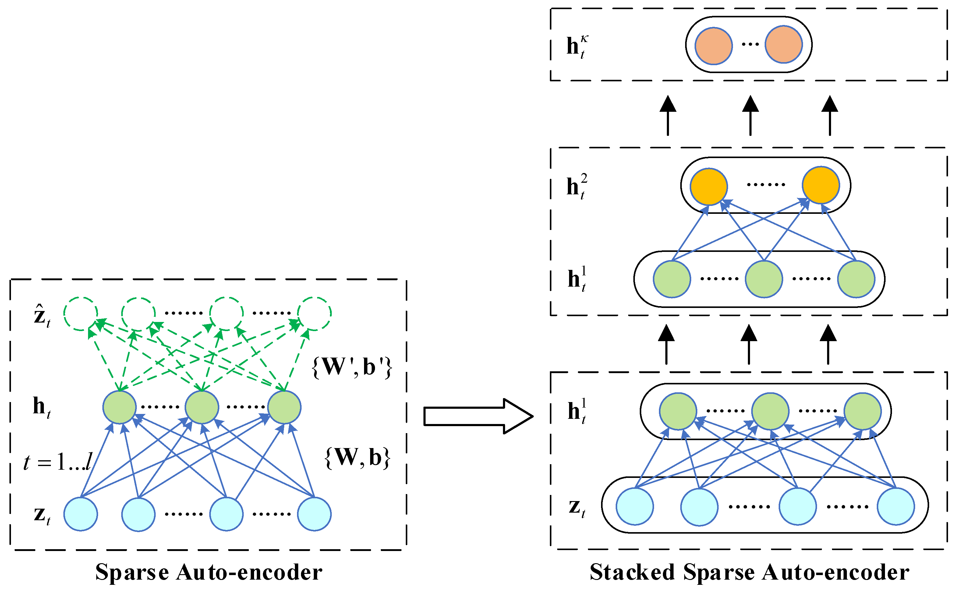
4.2. Stacked Auto-Encoder

After the measurements $y_t\in {ℝ}^{n_y}$ are decomposed by VMD, the result is represented as $z_t\in {ℝ}^{n_y\times n_{vmd}}$, where $n_{vmd}$ presents the number of modes. In order to make a prediction, the dimensionality $n_y\times n_{vmd}$ of VMD decomposition modes will be reduced to a single HI $h\in R^1$ by the stacked sparse auto-encoder (SSAE) here.

An auto-encoder (AE) is a type of neural network that typically consists of an encoder and a decoder, which can have multiple layers, with the number of layers varying depending on the specific implementation [30]. A sparse auto-encoder (SAE) is an extension of the basic AE, where a sparsity constraint is added to the hidden layers. This constraint ensures that, even when the hidden layer contains many neurons, the network is still able to extract the essential features and structure of the input data. Sparsity is typically enforced by regularizing the activations of the hidden layer, encouraging most of the neurons to remain inactive (close to zero) while only a small subset is active at any time. This leads to a more efficient representation of the input data. The structure of an SAE is shown in Figure 1, where the actual output of the SAE is represented as h, the sparse activation vector [31].

As shown in Figure 1, the SSAE obtains multiple layers by stacking the hidden layer of the underlying SAE as the input of the next layer, and the SSAE is uniformly trained to obtain a complete network. For the m-dimensional training sample $z_t=[z_t^1,z_t^2,\dots ,z_t^m]\in R^{1\times m}$ (t = 1, 2, …, l, l is the length of the training data), the SSAE firstly builds the first layer of the network, and the n₁-dimension output $h^1\in R^{n_1\times l}$ of the first layer is

$$h^1=f(W^{1}z+b^1)$$

(10)

where the dimension of z is $n_y\times n_{vmd}$, $W^{\upsilon }$ and $b^{\upsilon }$ are the weight matrix and bias vector of the υth layer, and $f(\bullet )$ is the activation function. The input of the second layer network is the output of the first layer network, so the n₂-dimensional output $h^2\in R^{n_2\times l}$ of the second layer network is calculated as follows:

$$h^2=f(W^2{h}^1+b^2)$$

(11)

Then, the output of the κth layer of the SSAE network is

$$\begin{array}{cc}{h}^{\kappa }& =f(W^{\kappa }{h}^{\kappa -1}+b^{\kappa })\hfill \\ & =f(W^{\kappa }f(W^{\kappa -1}{h}^{\kappa -2}+b^{\kappa -1})+b^{\kappa })\hfill \\ & \dots \dots \hfill \end{array}$$

(12)

Here, in order to obtain a single-dimensional HI for the prediction of the degradation trend, the output data dimension n¹, n², …, n^κ of each layer of the network decreases layer by layer until it becomes 1.

In SSAE training, all the weights and biases $\{W^1,b^1,\dots ,W^{\upsilon },b^{\upsilon },\dots ,W^{\kappa },b^{\kappa }\}$ of the stacked network are solved synchronously according to training the object function:

$$J_{sparse}(W,b,W^{\prime },b^{\prime })=J(W,b,W^{\prime },b^{\prime })+\beta {\displaystyle {\sum }_{j=1}^{n}KL(\rho ||{\widehat{\rho }}_j)}$$

(13)

where the sparse penalty term is selected by the relative entropy (KL divergence):

$$KL(\rho ||{\widehat{\rho }}_j)=\rho \log {\displaystyle \frac{\rho }{{\widehat{\rho }}_j}}+(1-\rho )\log {\displaystyle \frac{1-\rho }{1-{\widehat{\rho }}_j}}$$

(14)

and ${\widehat{\rho }}_j={\displaystyle \frac{1}{m}}{\displaystyle {\sum }_{i=1}^m[h_j(z_i)]}$ is the average activation of hidden neurons j. $\rho$ is the sparsity parameter, which is a small value close to 0. The constraint ${\widehat{\rho }}_j=\rho$ is enforced during the training. If this constraint is satisfied, the hidden activities must mostly be close to 0.

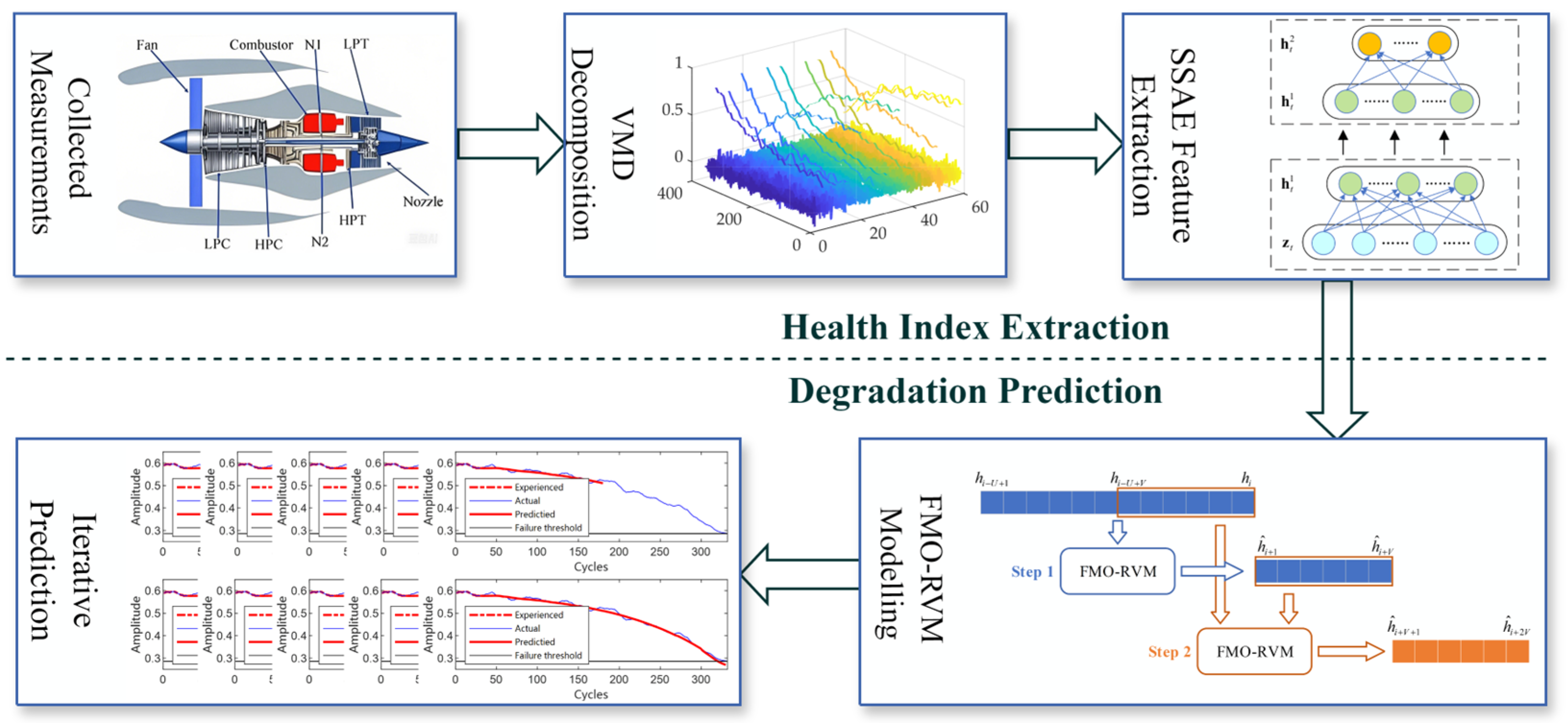
5. The Proposed Prognostic Method

5.1. Fast Prediction by Multi-Output Relevance Vector Regression

When single-output RVM is applied for predictions, $d_i\in {ℝ}^{U\times 1}$ in Equation (1) represents the HI at time i and U − 1 moments before it $[h_{i-U+1},\dots ,h_{i-1},h_i]$, and $t_i\in {ℝ}^{1\times V}$ (here, V = 1 for single-output RVM) represents the single-step forward prediction h_i+1. In this case, the data at the current time and the previous time are used to predict the data at the current time:

$${\widehat{h}}_{i+1}=\mathrm{P}(h_{i-U+1},\dots ,h_{i-1},h_i)$$

(15)

where $\mathrm{P}$ presents the single-output RVM regression algorithm. The main purpose of the multi-step fault predictor was to utilize historical health information to predict the health status level of the system and provide the corresponding confidence interval. As the simple RVM can only realize single-point predictions, moving-window technology was chosen to establish the continuous prediction model [32]. Specifically, for long-term predictions, the data ${\widehat{h}}_{i+1}$ at time i + 1 obtained by the prediction should be taken as the input for predicting the data ${\widehat{h}}_{i+2}$ at time i + 2. Then, ${\widehat{h}}_{i+1}$ and ${\widehat{h}}_{i+2}$ can be used as the input for predicting ${\widehat{h}}_{i+3}$, and so on:

$$\begin{array}{l}{\widehat{h}}_{i+2}=\mathrm{P}(h_{i-U+2},\dots ,h_i,{\widehat{h}}_{i+1})\\ {\widehat{h}}_{i+3}=\mathrm{P}(h_{i-U+3},\dots ,,{\widehat{h}}_{i+1}{\widehat{h}}_{i+2})\\ \dots \dots \\ {\widehat{h}}_{i+\tau }=\mathrm{P}(h_{i-U+\tau },\dots ,{\widehat{h}}_{i+\tau -2},{\widehat{h}}_{i+\tau -1})\end{array}$$

(16)

For long-term predictions through single-output RVM, if a τ time prediction is required, τ iterations are required. When τ is large, the operation takes a long time. Fortunately, the FMO-RVM can solve this problem. When the FMO-RVM is utilized to build a prediction model, the iterative process of Equation (16) becomes

$$\begin{array}{l}{\widehat{h}}_{i+1},\dots ,{\widehat{h}}_{i+V}=\mathrm{P}\mathrm{M}(h_{i-U+1},\dots ,h_{i-1},h_i)\\ {\widehat{h}}_{i+V+1},\dots ,{\widehat{h}}_{i+2V}=\mathrm{P}\mathrm{M}(h_{i-U+V},\dots ,{\widehat{h}}_{i+1},\dots ,{\widehat{h}}_{i+V})\\ {\widehat{h}}_{i+2V+1},\dots ,{\widehat{h}}_{i+3V}=\mathrm{P}\mathrm{M}(h_{i-U+2V},\dots ,{\widehat{h}}_{i+V+1},\dots ,{\widehat{h}}_{i+2V})\\ \dots \dots \\ {\widehat{h}}_{i-V+1+\tau },\dots ,{\widehat{h}}_{i+\tau }=\mathrm{P}\mathrm{M}({\widehat{h}}_{i-2V+1+\tau },\dots ,{\widehat{h}}_{i-V+\tau -1},{\widehat{h}}_{i-V+\tau })\end{array}$$

(17)

where $\mathrm{P}\mathrm{M}$ is the FMO-RVM regression process. In this case, the predicted value of length V will be estimated by a single iteration process. Furthermore, the predicted value at the next time V can be obtained by substituting the predicted value at i + 1 to i + V into the input for the iteration, that is, the predicted value ${\widehat{h}}_{i+V+1}$ to ${\widehat{h}}_{i+2V}$. Therefore, if a τ-step forward prediction is needed, only $⌈\tau /V⌉$ calculations are needed, with $⌈•⌉$ indicating upward rounding.

5.2. The Proposed Prognostic Structure

Aiming at the complex system of multi-sensor measurements, this study proposes an HI extraction method based on VMD and an SSAE and adopted the FMO-RVM to realize the learning and prediction of the degradation trend. The basic structure is shown in Figure 2, and the specific steps are as follows:

• Step 0. Sensor measurement data are collected.
• Step 1. The measurement data are split into training and test sets, and the training set is normalized. The normalization process uses Gaussian normalization, where each feature is scaled to have a zero mean and unit variance.
• Step 2. The features of the measurement data are decomposed by VMD.
• Step 3. The features decomposed by VMD are subjected to a data dimensionality reduction through the SSAE, and a comprehensive HI is extracted.
• Step 4. The training set is prepared and used to train the predictor based on the FMO-RVM.
• Step 5. The trained predictor based on the FMO-RVM is employed to predict the degradation trend and the remaining useful life.

In this paper, the input and output dimensions were both q for FMO-RVM regression modeling. When the total length of the training data is l, the input–output sequence pair constructed according to Equation (17) is as follows:

$$\begin{array}{l}{h}_1,\dots ,h_q\to h_{q+1},\dots ,h_{2q}\\ h_2,\dots ,h_{q+1}\to h_{q+2},\dots ,h_{2q+1}\\ h_3,\dots ,h_{q+2}\to h_{q+3},\dots ,h_{2q+2}\\ \dots \\ h_{l-2q},\dots ,h_{l-q-1}\to h_{l-q},\dots ,h_{l-1}\\ h_{l-2q+1},\dots ,h_{l-q}\to h_{l-q+1},\dots ,h_l\end{array}$$

(18)

where the input length for training the model is l − 2q + 1. The multi-output regression model of the FMO-RVM is established by training input–output pairs with the number of l − 2q + 1.

6. Case Study 1

6.1. Brief Introduction of Aeroengine Performance Simulation Data (C-MAPSS)

In order to solve the problem that the data-driven prediction system lacks run-to-failure data, NASA established an aeroengine prediction database to verify the prediction algorithm [33]. The simulation software C-MAPSS (version 1.0) is used to build a simulation model of a large aircraft turbofan engine. The inputs to the C-MAPSS model include the fuel flow as well as the fans, low-pressure compressor (LPC), high-pressure compressor (HPC), high-pressure turbine (HPT), and low-pressure turbine (LPT); the flow; the efficiency; and the pressure ratio of the five rotating parts. The output simulation data of the aeroengine for testing included the output performance parameters of five rotating components.

In the study, 21 output measurement data points were used, including the pressure, temperature, engine pressure ratio, rotational speed, flow ratio, seepage rate, etc. The specific sensor measurement data can be found in [33]. These outputs contain various sensor response surfaces and operability margins, and researchers can observe the operating state of the engine by looking at these 21 sets of measurements. This dataset provides a set of run-to-failure data for HP compressor performance degradation, modelling engine performance degradation due to wear and not targeting any specific failure.

6.2. Process and Results of Health Index Extraction Method

To obtain as many training samples as possible, the aeroengine run-to-failure data with the longest period in the dataset were selected as the training data. However, since the 21 measurements had operability margins and were simulated under operating conditions of different flight altitudes, TRAs, and Mach numbers, the measurements needed to be pre-processed and extracted to obtain the HI for condition monitoring. The extraction of the HI was carried out according to the following steps:

(i)

Data standardization. The formula is N(y^d) = (y^d − μ^d)/σ^d, where y^d is the d-dimensional feature data of the training set of the measurement data sample, d = {1, 2,…, 21}, and μ^d and σ^d are the mean and standard deviation of y^d, respectively. The specific sensor measurement data are shown in

Table 1. Measurements of the aeroengine degradation datesets.

Variable	Description	Units	Variable	Description	Units
T2	Fan inlet total temperature	°R	Phi	Ratio of fuel flow to Ps3	pps/psi
T24	Total pressure at LPC outlet	°R	NfR	Corrected fan speed	rpm
T30	Total pressure at HPC outlet	°R	NcR	Corrected core speed	rpm
T50	Total pressure at LPT outlet	°R	BPR	Bypass ratio	\
P2	Pressure at fan inlet	psia	farB	Burner fuel–air ratio	\
P15	Total pressure in bypass duct	psia	htBleed	Bleed enthalpy	\
P30	Total pressure at HPC outlet	psia	Nf_dmd	Demanded fan speed	rpm
Nf	Physical fan speed	rpm	PCNfR_dmd	Corrected fan speed demanded	%
Nc	Physical core speed	rpm	W31	HPT coolant bleed	lbm/s
EPR	Engine pressure ratio (P50/P2)	\	W32	LPT coolant bleed	lbm/s
Ps30	Static pressure at HPC outlet	psia

. These outputs contain various sensor response surfaces and operability margins, and researchers can observe the operating state of the engine by looking at these 21 sets of measurements.

(ii)

VMD decomposition. The 12 groups of measurements obtained from the screening were decomposed by VMD; the modal number of VMD was 5. This number was chosen after experimentation to strike a balance between effective decomposition and computational efficiency. The training data decomposed by VMD are shown in Figure 3. Modes 1–4 mainly contain noise data, and mode 5 preserves the main degradation trend.

(iii)

Extraction using SSAE. The comprehensive characteristic index was obtained as the predicted HI. Here, 60-dimensional data needed to be compressed to 1-dimensional data through an SSAE.

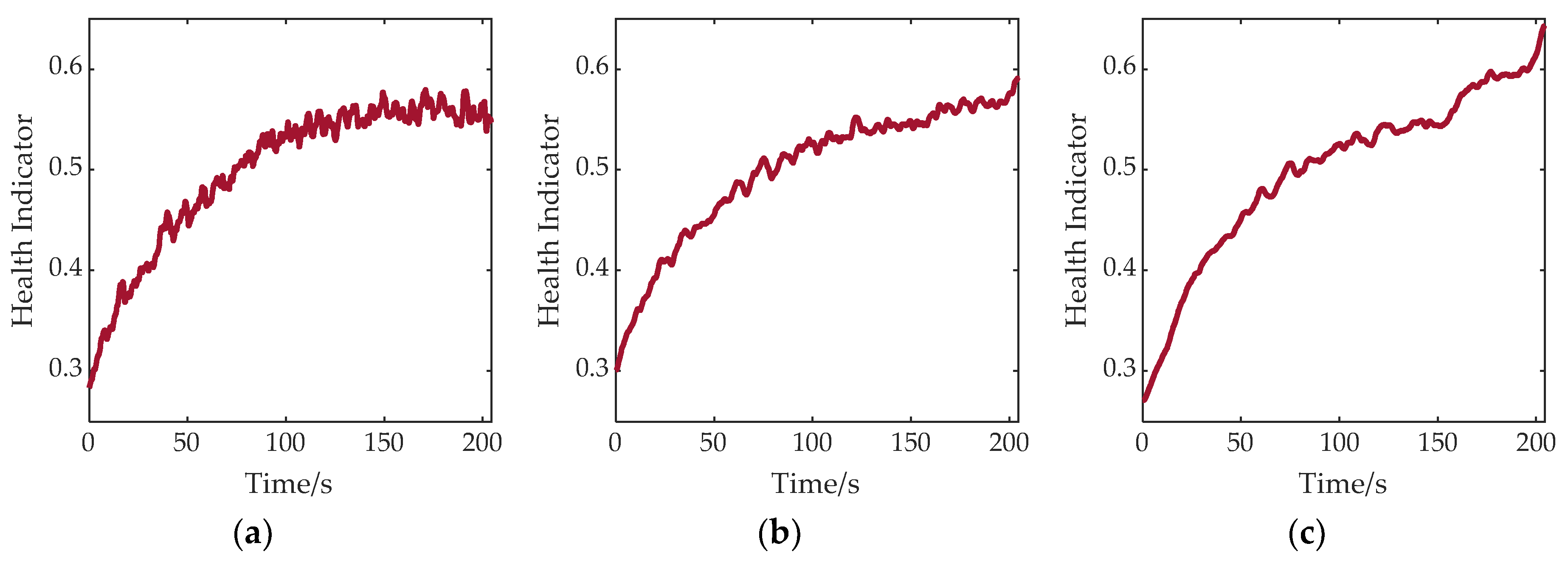
6.3. Performance Verification of Health Index Extraction Based on VMD-SSAE

At first, the effect of VMD on the extraction of the HI was verified. In Figure 4a, the PCA dimension reduction after VMD decomposition (called VMD+PCA) and the PCA dimension reduction directly on the normalized data (called PCA) are compared; the SSAE dimensionality reduction after VMD decomposition (called VMD+SSAE) and the SSAE dimensionality reduction directly on the normalized data (called SSAE) were also compared. By adding VMD, the interference of noise data on the HI was eliminated, and the ability of noise reduction was added to the data dimensionality reduction method.

Then, the ability of the HI extraction methods by the PCA and SSAE were further compared. It can be seen from Figure 4a that, under these training data, there was no significant difference between the HI extracted by the PCA and that extracted by the SSAE. Therefore, other test data are provided here. In order to clarify the state of the data, the running ratio $\gamma$ was defined as follows:

$$\gamma ={\displaystyle \frac{l_{\mathit{past}}}{l_{\mathit{past}}+l_{\mathit{RUL}}}}={\displaystyle \frac{l_{\mathit{past}}}{l_{\mathit{run}-\mathit{to}-\mathit{failure}}}}$$

(19)

where l_past represents the length of the existing process test data, l_RUL is the actual remaining life, and l_{run-to-failure} is the full-life operating cycle. $\gamma$ is used to represent the proportion of the measured data to the length of all the runs to failure. The eight groups of test data in

Table 2. Basic parameters of the test dataset for the degradation process.

Test Data Number	lpast (Cycles)	lRUL (Cycles)	$\mathit{\gamma }$
Test data 1	303	21	93.52%
Test data 2	232	54	81.12%
Test data 3	198	11	93.52%
Test data 4	101	63	61.59%
Test data 5	97	137	41.45%
Test data 6	75	79	48.70%
Test data 7	50	106	32.05%
Test data 8	31	112	21.68%

contain different values for l_past, l_RUL, and the running ratio $\gamma$, which can basically represent all types of test data.

When the degradation process of the test data is relatively complete (ρ is larger), as shown in Figure 4a–c, a PCA can extract the HI well. However, when the degradation process is in the early stage (ρ is small), as shown in Figure 4d–f, a PCA cannot extract the degradation trend well when extracting the HI. But the HI extracted by the SSAE can reflect the degradation trend of the performance relatively well.

When comparing Figure 4c,d, although the length of test data 5 was longer than that of test data 6, its running ratio ρ was smaller. Therefore, a PCA’s ability to extract the HI for data 5 is not as good as that for data 6, while the SSAE did not have this problem.

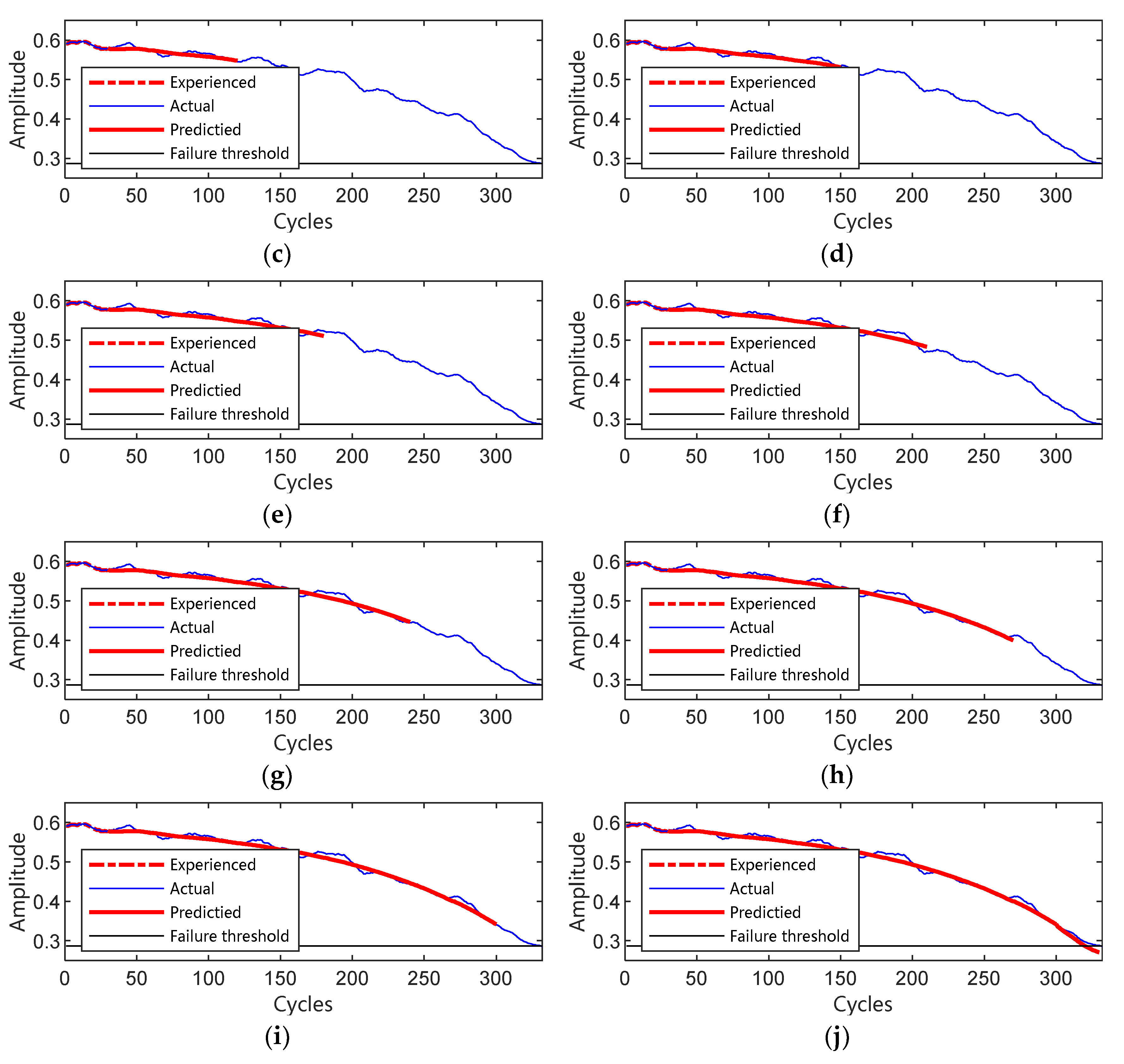
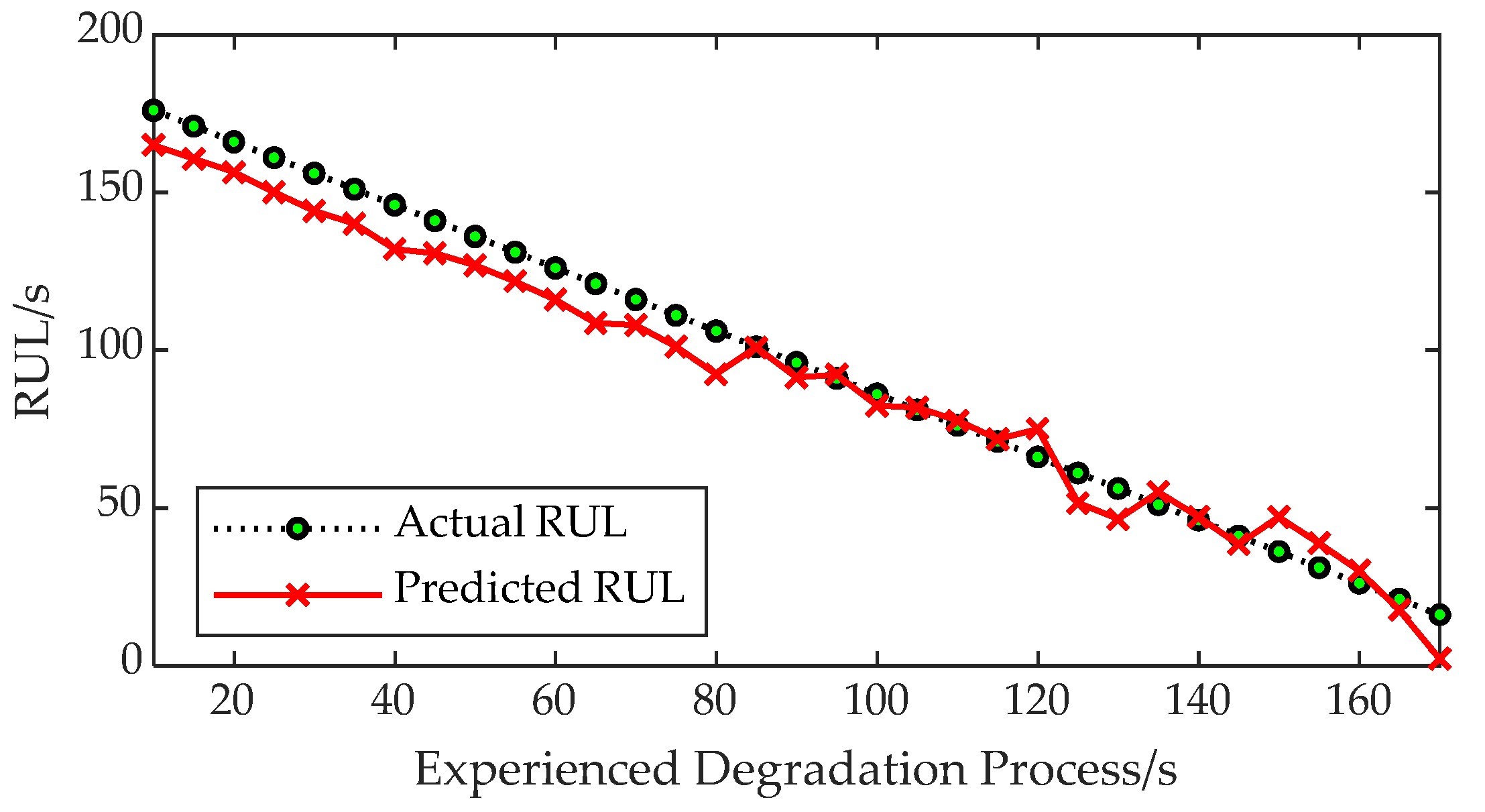
6.4. Performance Verification of Remaining Life Prediction Based on FMO-RVM

The prediction curves based on the FMO-RVM, which correspond to 10 iterations, are shown in Figure 5. The total length of the test data was 362 cycles, and the actual remaining life was 302 cycles. At this time, the input and output data dimension of the FMO-RVM used for training was 30, so 300 time periods of prediction can be achieved with only 10 iterations. In Figure 5j, the predicted data exceeds the failure threshold, the system was determined to fail at this time, and the iteration stops. The estimated remaining life by the FMO-RVM was 295, which differed from the actual remaining life by seven cycles. Overall, the FMO-RVM method is accurate in estimating the trend of the data.

To further verify the regression prediction ability of the FMO-RVM, the FMO-RVM was compared with a traditional SVM and RVM. The training data were still used for testing here. The total degradation process length of these data was 362, and the degradation process length that occurred ranged from 60 to 300 in steps of 10. The prediction accuracy of the SVM, RVM, and FMO-RVM was compared under different lengths of existing process data. Here, the prediction accuracy was measured using the mean absolute error (MAE), mean squared error (RMSE), and coefficient of determination (R²). The calculation formula of R² is as follows:

$$R^2=1-{\displaystyle \frac{{\displaystyle {\sum }_{i=1}^N{(y-\widehat{y})}^2}}{{\displaystyle {\sum }_{i=1}^N{(y-\overline{y})}^2}}}$$

(20)

and the calculation formula of RMSE is as follows:

$$\mathrm{RMSE}=\sqrt{{\displaystyle \frac{1}{N}}{\displaystyle {\sum }_{i=1}^N{({\widehat{y}}_i-y_i)}^2}}$$

(21)

During training, the input dimension of the single-output SVM and RVM was 30, and the output dimension was 1. The input and output data dimensions of the FMO-RVM were both 30, and linear kernels were used. The results are shown in Figure 6. For the test data, the prediction accuracy of the SVM was the lowest, with an average of only 77.66%; in particular, when the existing process data points numbered 230, it was only 38.51%. The RVM regression accuracy was better than that of the SVM, reaching 96.88%, and the lowest value also appeared for 230 process data points, which was 88.52%. The FMO-RVM was the best, with an average of 97.93%, reaching 98.76% with 230 process data points. Since both the RVM and SVM output a single dimension, the prediction time of these two methods was much larger than that of the FMO-RVM, and the estimated time was about 30 times. Therefore, the FMO-RVM was better than the RVM and SVM in terms of the regression accuracy of the predicted data.

7. Case Study 2

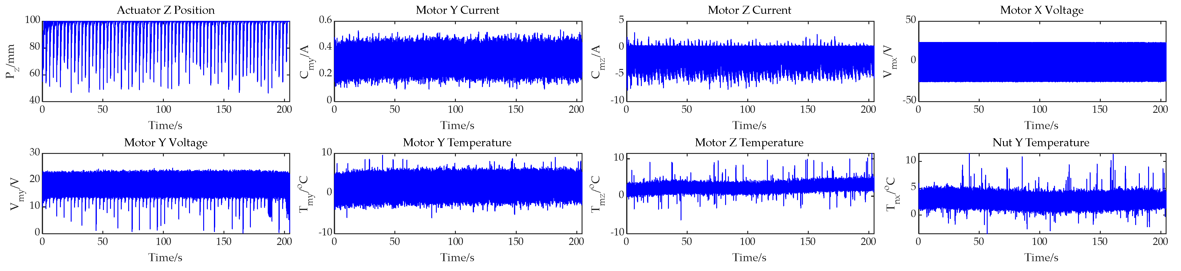
7.1. Brief Introduction of Electro-Mechanical Actuator

Electro-mechanical actuators (EMAs), serving as critical components in aircraft electronic control systems, are among the most widely utilized actuators in aerospace engineering due to their paramount importance for flight safety [34]. In 2000, the National Aeronautics and Space Administration (NASA) established an autonomous, lightweight testbed at the Dryden Research Center—the flyable electro-mechanical actuator (FLEA) system [35,3637], as illustrated in Figure 7a. The testbed incorporates EMAs manufactured by the Ultra Motion Corporation (Figure 7b), featuring key performance specifications that include a maximum velocity of 20 feet per second; a peak drive force capability of 500 pounds; bidirectional repeatability within ±0.0003 inches; and unidirectional repeatability achieving ±0.0001 inches. During a flight simulation, the load path automatically transitions between healthy and faulted actuators through a redundant switching mechanism. This innovative setup enables the synchronized acquisition of both nominal and degraded sensor data under identical operational conditions, thereby facilitating a comprehensive failure mode analysis and the validation of fault-tolerant control algorithms.

The FLEA introduces a blockage fault, denoted as a “jam”, by modifying the return channel of the ball screw mechanism. This is achieved by inserting an advanceable fixed screw into the return channel that partially or completely obstructs its flow. This obstruction prevents the normal circulation and rotation of the balls, transforming the ball screw from a high-efficiency friction mechanism into one with a lower efficiency, resembling that of a conventional lead screw.

Measurement data are collected from multiple output sensors corresponding to the flight conditions, including the load, position, temperature, current, and voltage. The specific sensor names and their main parameters are listed in

Table 3. Prognostic sensor parameters of EMAs.

Sensor	Abbr.	Unit	Sensor	Abbr.	Unit
Actuator Z Position	Pz	mm	Motor Y Voltage	Vmy	V
Measured Load	L	lb	Motor X Temperature	Tmx	°C
Motor X Current	Cmx	A	Motor Y Temperature	Tmy	°C
Motor Y Current	Cmy	A	Motor Z Temperature	Tmz	°C
Motor Z Current	Cmz	A	Nut X Temperature	Tnx	°C
Motor X Voltage	Vmx	V	Nut Y Temperature	Tny	°C

. The temperature is monitored using thermocouples installed in the nut and motor. The test data are acquired using the NI 6259 data acquisition card at a sampling frequency of 1 kHz. The digital acquisition card has a resolution of 32 bits. Detailed testbed data can be found in the referenced literature [38].

This section selects test data on the transition from a blockage (jam) to failure in the return channel of the electro-mechanical actuator (EMA) used in aviation controllers. The occurrence of a jam is attributed to increased friction caused by the jamming of the ball screw nut, which results in additional current being directed to the test actuator by the controller. This, in turn, leads to the gradual accumulation of heat inside the engine casing. Overheating eventually causes damage to the winding insulation, followed by a short circuit, ultimately resulting in failure [30]. The motion profile is a sinusoidal curve with an amplitude of 80 mm, a frequency of 0.5 Hz, and a maximum velocity of 0.08 m/s.

The measurement data collected by the measurement sensors are shown in Figure 8.

As the system warms up, the temperature typically increases gradually and stabilizes at a relatively constant level. However, any abnormal or rapid temperature rise, especially under steady load conditions, may indicate potential faults such as internal friction or mechanical degradation. This is particularly evident in the X-axis motor temperature and X-axis nut temperature, where significant temperature increases were observed. Meanwhile, data anomalies occurring at the moment of system failure can be identified from the X-axis motor current and Y-axis motor voltage. These anomalies, often characterized by irregular spikes or dips, help pinpoint the exact moment when the system begins to fail.

However, a large amount of noise and invalid data still exist in all the measurement data. These data cannot be directly applied to performance monitoring. Merely deleting seemingly invalid data based on experience may lead to the possibility of losing deeper information. Therefore, feature classification and extraction methods need to be adopted to obtain healthy indicator data that can be used for condition detection.

7.2. Prediction Performance of FMO-RVM in EMA Dataset

Here, the single-channel health indicators obtained through a VMD+SSAE dimensionality reduction under different numbers of modes were compared, as shown in Figure 9. It can be seen that, when the number of modes was small (e.g., five), the extracted health indicator retained a significant amount of noise, and the upward trend in the final stage was not clearly represented. On the other hand, when the number of modes was large (e.g., 20), the extracted health indicator became overly smooth due to the loss of certain features. Therefore, considering all factors, this algorithm ultimately selected 10 modes for the prediction application of the EMA.

To further validate the performance of the predictive regression model proposed in this chapter, a multi-input multi-output long short-term memory (LSTM) network, which has shown outstanding performance in time series modeling, was used as a comparative algorithm. Both the input and output data lengths were set to 50, and the experimental results are shown in Figure 10. The failure threshold was defined as the mean value of the health indicator near the moment when the X-axis motor current exhibited abnormal behavior, which was 0.5728. It was observed that the LSTM tended to overestimate the upward trend during predictions, which would result in the predicted remaining useful life being significantly shorter than the actual remaining useful life. In contrast, the FMO-RVM method proposed in this chapter showed a prediction curve that was consistent with the trend of the actual operating curve. Therefore, the accuracy of the predicted remaining useful life was also higher.

Figure 11 shows the comparison results between the remaining useful life prediction results of the prediction algorithm proposed in this chapter and the actual remaining useful life. The length of the existing process data ranged from 10 s to 170 s, and the corresponding actual remaining useful life ranged from 176 s to 16 s. It can be seen that, even when there was only 10 s of process data at the beginning, the predicted remaining useful life still had a high accuracy. When the process data were around 80 s to 140 s, the predicted remaining useful life was the most accurate. When the process data were from 150 s to 160 s, the prediction deviation was the largest, but it was still within a relatively small range and was corrected in the last segment. Taking all time periods into account, the algorithm proposed in this section can predict the remaining useful life well with a high accuracy.

8. Conclusions and Discussion

In order to improve the efficiency and accuracy of residual life predictions for complex systems such as aeroengines, a long-term prediction algorithm based on the FMO-RVM was proposed in this paper. Through the experiments conducted in a widely used and researched simulation run-to-failure database established at NASA for aeroengines and EMAs, the performance of the predictive architecture presented in this paper was verified. Firstly, an extraction method without prior knowledge was proposed using VMD and an SSAE to obtain the HI; it performed better in extracting the HI than a PCA and shallow network. Then, through obtaining multi-time prediction results through a single-step operation, the prediction method based on FMO-RVM regression proposed in this paper resulted in a reduced prediction quantity; in addition, compared with the SVM, RVM, and LSTM methods, the prediction method proposed in this paper had a higher prediction accuracy.

The following conclusions can be drawn from this study:

• The deep sparse auto-encoder demonstrates superior feature extraction capabilities compared to the single-layer sparse auto-encoder. When combined with variational mode decomposition, it effectively extracted implicit health indicators from sensor measurements. Compared to a traditional PCA, the feature extraction ability of the deep sparse auto-encoder is significantly enhanced.
• The proposed FMO-RVM prediction method exhibited a higher accuracy than the SVM, RVM, and LSTM methods. The composite kernel structure offers a greater stability compared to single kernels. Additionally, the multi-output approach not only improves the modeling and prediction accuracy, but also significantly reduces the computational time for predictions. This provides a favorable premise for the application of the algorithm in engineering practices.
• The algorithm was applied to the NASA engine and EMA degradation simulation dataset, which has been extensively utilized and validated, demonstrating significant generalizability. The prediction method proposed in this paper is capable of quickly and accurately estimating the remaining useful life. The results validate the proposed prediction scheme’s ability to provide rapid life prediction for complex systems, indicating its potential for expanded applications to a broader range of objects in the future.

References

1. Goebel, K.; Daigle, M.J.; Saxena, A.; Roychoudhury, I.; Sankararaman, S.; Celaya, J.R. Prognostics: The science of making predictions. Prognostics 2017, 1, 1–14. [Google Scholar]
2. Guo, J.; Li, Z.; Li, M. A Review on Prognostics Methods for Engineering Systems. IEEE Trans. Reliab. 2020, 69, 1110–1129. [Google Scholar] [CrossRef]
3. Tahan, M.; Tsoutsanis, E.; Muhammad, M.; Abdul Karim, Z.A. Performance-Based Health Monitoring, Diagnostics and Prognostics for Condition-Based Maintenance of Gas Turbines: A Review. Appl. Energy 2017, 198, 122–144. [Google Scholar] [CrossRef]
4. Qian, Y.; Yan, R.; Gao, R.X. A Multi-Time Scale Approach to Remaining Useful Life Prediction in Rolling Bearing. Mech. Syst. Signal Process. 2017, 83, 549–567. [Google Scholar] [CrossRef]
5. Khelif, R.; Chebel-Morello, B.; Malinowski, S.; Laajili, E.; Fnaiech, F.; Zerhouni, N. Direct Remaining Useful Life Estimation Based on Support Vector Regression. IEEE Trans. Ind. Electron. 2017, 64, 2276–2285. [Google Scholar] [CrossRef]
6. Wu, Y.; Yuan, M.; Dong, S.; Lin, L.; Liu, Y. Remaining Useful Life Estimation of Engineered Systems Using Vanilla LSTM Neural Networks. Neurocomputing 2018, 275, 167–179. [Google Scholar] [CrossRef]
7. Xu, D.; Sui, S.-B.; Zhang, W.; Xing, M.; Chen, Y.; Kang, R. RUL Prediction of Electronic Controller Based on Multiscale Characteristic Analysis. Mech. Syst. Signal Process. 2018, 113, 253–273. [Google Scholar] [CrossRef]
8. Li, X.; Ding, Q.; Sun, J.-Q. Remaining Useful Life Estimation in Prognostics Using Deep Convolution Neural Networks. Reliab. Eng. Syst. Saf. 2018, 172, 1–11. [Google Scholar] [CrossRef]
9. Jouin, M.; Gouriveau, R.; Hisel, D.; Pééra, M.-C.; Zerhouni, N. Particle Filter-Based Prognostics: Review, Discussion and Perspectives. Mech. Syst. Signal Process. 2016, 72, 2–31. [Google Scholar] [CrossRef]
10. Sankararaman, S.; Goebel, K. Uncertainty in prognostics and systems health management. Int. J. Progn. Health Manag. 2020, 6, 4. [Google Scholar] [CrossRef]
11. Bender, A. A multi-model-particle filtering-based prognostic approach to con-sider uncertainties in RUL predictions. Machines 2021, 9, 210. [Google Scholar] [CrossRef]
12. Park, H.; Kim, N.; Choi, J. Prognosis using bayesian method by incorporating physical constraints. In Proceedings of the Asia Pacific Conference of the PHM Society, Tokyo, Japan, 11–14 September 2023; Volume 4. [Google Scholar] [CrossRef]
13. Tseremoglou, I.; Bieber, M.; Santos, B.; Verhagen, W.; Freeman, F.; Kessel, P. The impact of prognostic uncertainty on condition-based maintenance scheduling: An in-tegrated approach. In Proceedings of the AIAA AVIATION 2022 Forum, Chicago, IL, USA, 27 June–1 July 2022. [Google Scholar] [CrossRef]
14. Caesarendra, W.; Widodo, A.; Thom, P.H.; Yang, B.S.; Setiawan, J.D. Combined Probability Approach and Indirect Data-Driven Method for Bearing Degradation Prognostics. IEEE Trans. Reliab. 2011, 60, 14–20. [Google Scholar] [CrossRef]
15. Zhou, Y.; Huang, M.; Chen, Y.; Tao, Y. A Novel Health Indicator for On-Line Lithium-Ion Batteries Remaining Useful Life Prediction. J. Power Sources 2016, 321, 1–10. [Google Scholar] [CrossRef]
16. Lin, Y.H.; Li, G.H. A Bayesian Deep Learning Framework for RUL Prediction Incorporating Uncertainty Quantification and Calibration. IEEE Trans. Ind. Inform. 2022, 18, 7274–7284. [Google Scholar] [CrossRef]
17. Tang, J.; Zheng, G.H.; He, D.; Ding, X.X.; Huang, W.B.; Shao, Y.M.; Wang, L.M. Rolling bearing remaining useful life prediction via weight tracking relevance vector machine. Meas. Sci. Technol. 2021, 32, 024006. [Google Scholar] [CrossRef]
18. Borchani, H.; Varando, G.; Bielza, C.; Larrañaga, P. A survey on multi-output regression. Wiley Interdiscip. Rev. Data Min. Knowl. Discov. 2015, 5, 216–233. [Google Scholar] [CrossRef]
19. Wang, Y.Z.; Xie, B.; E, S.Y. Adaptive relevance vector machine combined with Markov-chain-based importance sampling for reliability analysis. Reliab. Eng. Syst. Saf. 2022, 220, 108287. [Google Scholar] [CrossRef]
20. Safari, M.J.S.; Rahimzadeh Arashloo, S.; Vaheddoost, B. Fast Multi-Output Relevance Vector Regression for Joint Groundwater and Lake Water Depth Modeling. Environ. Model. Softw. 2022, 154, 105425. [Google Scholar] [CrossRef]
21. Cherkassky, V. The Nature of Statistical Learning Theory. IEEE Trans. Neural Netw. 1997, 8, 1564. [Google Scholar] [CrossRef]
22. Tipping, M.E. The Relevance Vector Machine. In Proceedings of the 13th International Conference on Neural Information Processing Systems, Denver, CO, USA, 29 November 1999; MIT Press: Cambridge, MA, USA, 1999; pp. 652–658. [Google Scholar]
23. Thayananthan, A.; Navaratnam, R.; Stenger, B.; Torr, P.H.S.; Cipolla, R. Pose Estimation and Tracking Using Multivariate Regression. Pattern Recognit. Lett. 2008, 29, 1302–1310. [Google Scholar] [CrossRef]
24. Ha, Y.; Zhang, H. Fast Multi-Output Relevance Vector Regression. Econ. Model. 2019, 81, 217–230. [Google Scholar] [CrossRef]
25. Tipping, M.E. Sparse Bayesian Learning and the Relevance Vector Machine. J. Mach. Learn. Res. 2001, 1, 211–244. [Google Scholar] [CrossRef]
26. Vazquez, E.; Walter, E. Multi-Output Support Vector Regression. IFAC Proc. Vol. 2003, 36, 1783–1791. [Google Scholar] [CrossRef]
27. Dragomiretskiy, K.; Zosso, D. Variational Mode Decomposition. IEEE Trans. Signal Process. 2014, 62, 531–544. [Google Scholar] [CrossRef]
28. Bertsekas, D.P. Multiplier Methods: A Survey. IFAC Proc. Vol. 1975, 8, 351–363. [Google Scholar] [CrossRef]
29. Rockafellar, R.T. A Dual Approach to Solving Nonlinear Programming Problems by Unconstrained Optimization. Math. Program. 1973, 5, 354–373. [Google Scholar] [CrossRef]
30. Ng, A.Y.; Lee, H. Sparse autoencoder. In CS294A Lecture Notes; Stanford University: Stanford, CA, USA, 2011. [Google Scholar]
31. Wang, Y.; Yao, H.; Zhao, S. Auto-encoder based dimensionality reduction. Neurocomputing 2016, 184, 232–242. [Google Scholar] [CrossRef]
32. Xu, P.; Wei, G.; Song, K.; Chen, Y. High-Accuracy Health Prediction of Sensor Systems Using Improved Relevant Vector-Machine Ensemble Regression. Knowl.-Based Syst. 2021, 212, 106555. [Google Scholar] [CrossRef]
33. Liu, Y.; Frederick, D.K.; DeCastro, J.A.; Litt, J.S.; Chan, W.W. User’s Guide for the Commercial Modular Aero-Propulsion System Simulation (C-MAPSS); NASA: Washington, DC, USA, 2012. [Google Scholar]
34. Jensen, S.C.; Jenney, G.D.; Dawson, D. Flight Test Experience with An Electromechanical Actuator on the F-18 Systems Research Aircraft. In Proceedings of the Digital Avionics Systems Conference, Philadelphia, PA, USA, 7–13 October 2000; IEEE: Piscataway, NJ, USA, 2000. [Google Scholar]
35. Lin, Y.; Baumann, E.; Bose, D.M.; Beck, R.; Jenney, G. Tests and Techniques for Characterizing and Modeling X-43A Electromechanical Actuators; NASA: Washington, DC, USA, 2008. [Google Scholar]
36. Balaban, E.; Saxena, A.; Narasimhan, S.; Roychoudhury, I.; Goebel, K.F.; Koopmans, M.T. Airborne Electro-Mechanical Actuator Test Stand for Development of Prognostic Health Management Systems; NASA: Washington, DC, USA, 2010. [Google Scholar]
37. Koopmans, M.; Mattheis, C.; Lawrence, A. Electro Mechanical Actuator Test Stand for In-Flight Experiments; NASA: Washington, DC, USA, 2009. [Google Scholar]
38. Balaban, E.; Saxena, A.; Narasimhan, S.; Roychoudhury, I.; Koopmans, M.; Ott, C.; Goebel, K. Prognostic Health-Management System Development for Electromechanical Actuators. J. Aerosp. Inf. Syst. 2015, 12, 329–344. [Google Scholar] [CrossRef]
Figure 1. Schematic diagram of sparse auto-encoder and stacked sparse auto-encoder.
Processes 13 01232 g001
Figure 2. Schematic diagram of the proposed prognostic process.
Processes 13 01232 g002
Figure 3. Characteristic data obtained by VMD.
Processes 13 01232 g003
Figure 4. Comparison of SSAE and PCA feature extraction performance: (a) test data 1, (b) test data 3, (c) test data 6, (d) test data 5, (e) test data 7, and (f) test data 8.
Processes 13 01232 g004
Figure 5. Step-by-step prediction process by FMO-RVM: (a) the first iteration predicts 30 steps, (b) the second iteration predicts 60 steps, (c) the third iteration predicts 90 steps, (d) the forth iteration predicts 120 steps, (e) the fifth iteration predicts 150 steps, (f) the sixth iteration predicts 180 steps; (g) the seventh iteration predicts 210 steps, (h) the eighth iteration predicts 240 steps, (i) the nineth iteration predicts 270 steps, (j) the tenth iteration predicts 300 steps.
Processes 13 01232 g005aProcesses 13 01232 g005b
Figure 6. Comparison of error percentages for remaining life predictions based on SAE, RVM and SSAE.
Processes 13 01232 g006
Figure 7. Electro-mechanical actuator fault injection test system and test subjects. (a) Schematic of the FLEA testbed setup; (b) electro-mechanical actuator used in the testbed.
Processes 13 01232 g007
Figure 8. Measurement data on performance degradation of aviation electro-mechanical actuators under jam fault conditions.
Processes 13 01232 g008aProcesses 13 01232 g008b
Figure 9. Health indicators extracted under different numbers of modes: (a) number of modes = 5; (b) number of modes = 10; and (c) number of modes = 20.
Processes 13 01232 g009
Figure 10. Comparison of prediction abilities of multiple-input multiple-output time series models. (a) LSTM prediction with an existing process length of 10 s; (b) LSTM prediction with an existing process length of 100 s; (c) FMO-RVM prediction with an existing process length of 10 s; and (d) FMO-RVM prediction with an existing process length of 100 s.
Processes 13 01232 g010
Figure 11. The remaining useful life prediction results of the proposed FMO-RVM algorithm.
Processes 13 01232 g011