1. Introduction
Reliable access to electricity is one of the basic indicators for the quality of life and the economic standing of any community [
1,
2]. The availability of electricity directly affects living standards, education facilities, modes of transportation, industrial growth, and agriculture productivity [
3,
4]. Around 800 million people worldwide have no access to electricity, and a major part (approximately 83%) of this population belongs to rural areas [
3,
5]. The inhabitants of these underprivileged regions are still using fossil fuels, kerosene oil, and other raw materials to justify their basic energy needs, e.g., lighting, cooking, and heating [
3,
6]. Although these resources are partially fulfilling the very basic needs of the rural communities, however, these resources are not much environment friendly and also have adverse impacts on health [
3]. Therefore, electricity access to rural communities is the need of the hour to attain the associated socioeconomic benefits.
One possible way to electrify these unelectrified villages is through the expansion of the national electricity grid and associated generation, transmission, and distribution infrastructure. However, it involves a huge cost, and developing countries with limited resource availability cannot afford such large scale expansions [
3]. Alternately, distributed generation (DG) based microgrids have evolved as a reliable, affordable, and cost-effective solution for generation near to the load centers [
7,
8,
9]. Direct current (DC) microgrids, in comparison to alternating current (AC) microgrids, are considered more suitable for rural applications mainly due to (a) minimal synchronization requirements, (b) higher distribution efficiency, and c) no need of AC/DC power electronic conversion for interfacing with battery and solar photovoltaic (PV), as both are inherently DC in nature [
10,
11]. Additionally, the large scale market availability of highly efficient DC loads has further favored DC microgrids as a candidate choice for rural electrification [
12]. Since solar photovoltaic technology offers a clean, environment friendly, and green source of energy generation, therefore, this work is primarily focused on solar PV-based DC microgrids for sustainable rural electrification. Other distributed generation resources, e.g., diesel or hybrid PV/diesenl, are not considered within the current scope of this work.
During the last decade, a large number of solar PV-based DC microgrids have been deployed for rural electrification, particularly in India, Bangladesh, and African regions [
10,
13,
14,
15,
16,
17]. One prominent project is Mera Gao Power (MGP) in Uttar Pradesh (UP), India, which was founded in 2010 and is now considered as the lowest cost commercially viable solar PV- based DC microgrid. According to the reports, MGP has the potential to connect across 5000 villages, supplying basic electricity to approximately 50,000 households and 0.3 million rural consumers [
10,
18]. Similarly, The Energy and Resource Institute (TERI) of India under the campaign of lighting a billion lives provided electricity to 11,000 households in 243 villages spread across six states using solar DC microgrids [
10,
14]. Other considerable commercial examples are Sharatipur microgrid in Bangladesh and the Worldwide Fund for Nature (WWF) supported solar DC microgrid installed in Kasese district of Uganda by joint energy and environment project (JEEP) [
16,
17]. Despite the existence of many commercial projects, power architecture for these deployments is not standardized yet, and there exist many architecture variants. For instance, the MGP and the TERI project of India are using centralized architecture, in which the PV generation and battery storage resources are placed at a central location in the village, and from that central position, power is distributed at 24 V to each household. On the other hand, the Sharatipur project in Bangladesh is using a distributed architecture, where PV generation and battery storage resources are distributed throughout the village across various households. Other than these practical deployments, various other architectures have been proposed in the literature with scaled down laboratory-scale implementations. For instance, Madduri et al. [
19] proposed a scalable architecture using hybrid topology with PV generation at the central location, while battery storage resources are distributed across the village household. Similarly, Nasir et al. proposed a highly distributed architecture with neighborhood-level power-sharing capability implemented with decentralized control [
20,
21,
22]. The previous works mainly focus on design, analysis, and optimization of individual architectures without considering the impact of architectural variations on system sizing and losses [
1,
20,
21,
22,
23,
24,
25]. A framework for optimal planning and design of low power low voltage islanded DC microgrids for minimum upfront cost was developed in [
23]. Similarly, a framework for optimal planning and design of grid-connected DC microgrid was presented in [
25]. However, both of these works consider DC microgrid with central architecture and do not consider loss analysis and system sizing for other possible architectures. Distribution loss analysis for rural DC microgrids using modified Netwon–Raphson (NR) has been presented in [
1], while decentralized algorithms are discussed in [
20,
21,
26]. These works consider a distributed architecture of DC microgrid only and therefore do not illustrate insight on loss variations in other types of architectures. The comparison between central and distributed architectures has been performed in [
27], however, this work only considers distribution losses, ignoring the impact of variations in the converter losses. Alternatively, in this work, we present a compact framework to comprehensively analyze all the possible architectures along with both categories of losses, including distribution and conversion losses. The framework also presents the impact of losses on system sizing in various architectures, which is also an addition to the previous works in this domain. Therefore, this work is dedicated to the detailed comparison of all the possible architecture variants of DC microgrids for rural electrification implementations, with prime focus on losses, operational efficiency, and system sizing.
Our first contribution in this research work mainly includes the classification of various DC microgrid architectures employed for rural electrification. Based upon the existing deployments and proposed implementations, various architectures of DC microgrids are identified [
3,
10,
14,
15,
16,
17,
18,
19,
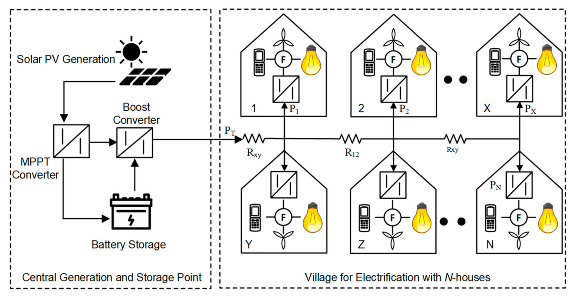
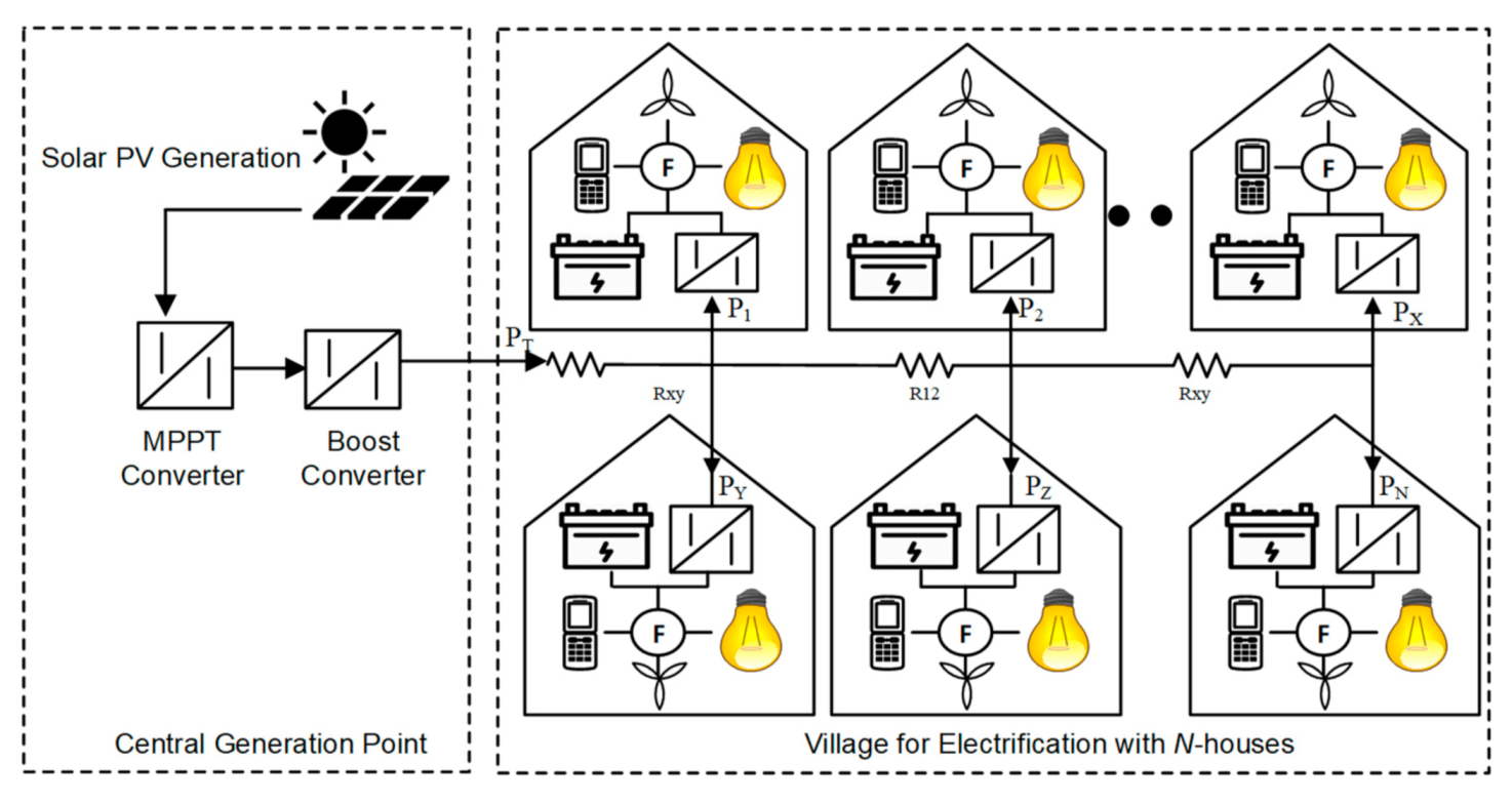
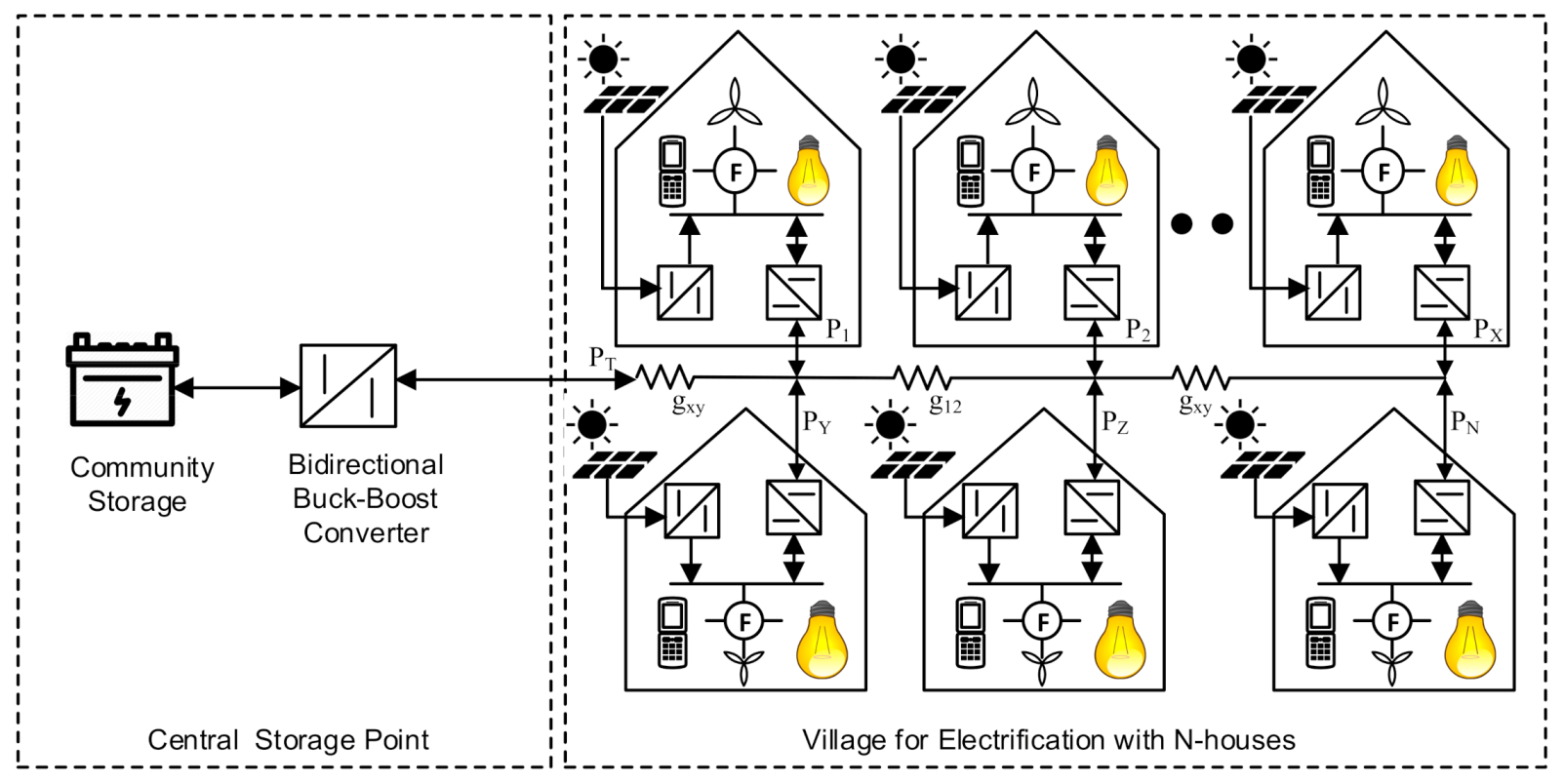
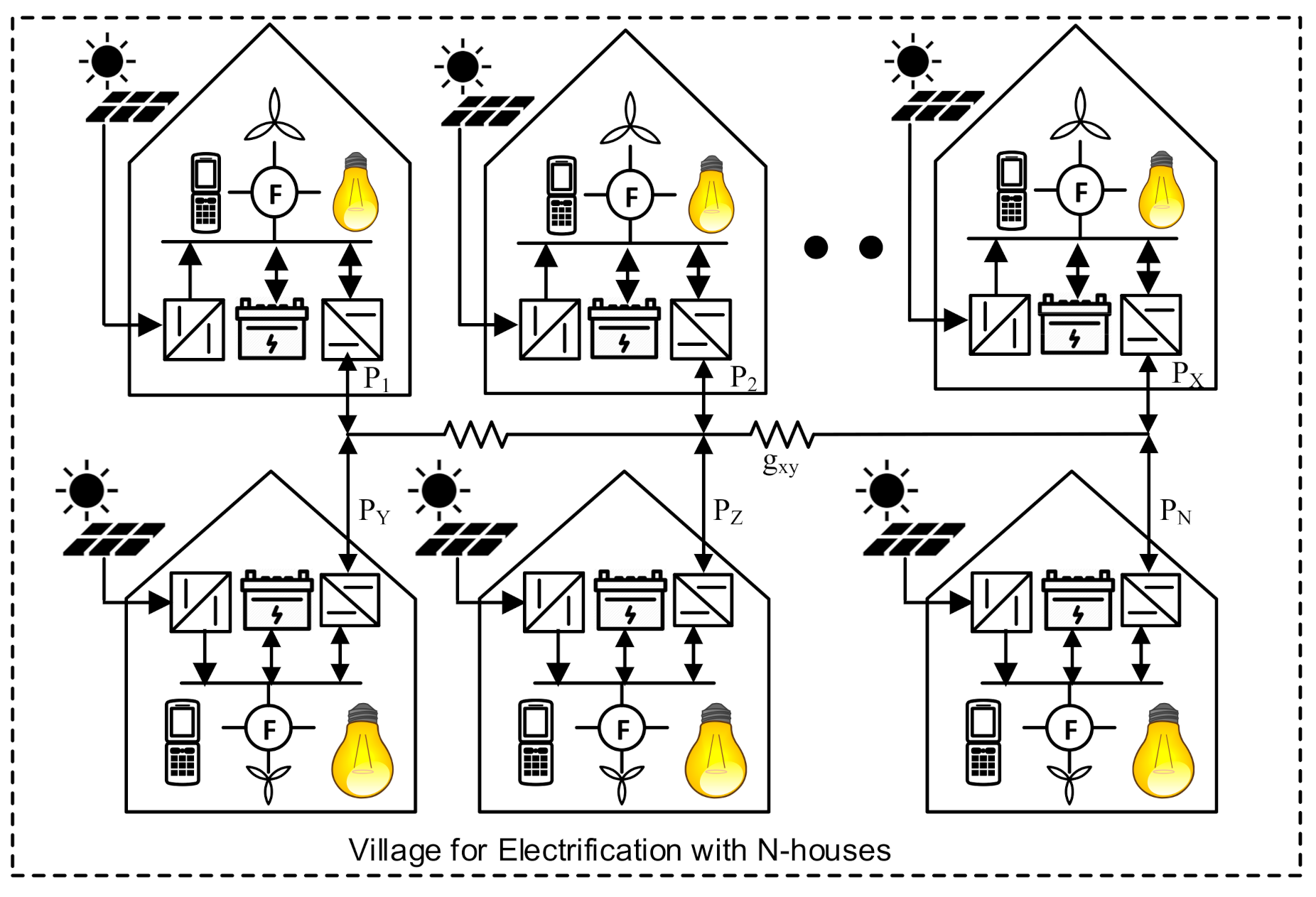
23]. These architectures are further classified based upon the placement of generation and storage resources and are termed as (a) central generation and central storage architecture (CGCSA), (b) central generation and distributed storage architecture (CGDSA), (c) distributed generation and central storage architecture (DGCSA), and (d) distributed generation and distributed storage architecture (DGDSA). The detailed power architectures, including component count and placement of resources for these architectures, are discussed in
Section 2.
Our second contribution mainly includes the identification and the quantification of various parameters that are coupled with the architectural design and impact the operational efficiency of the microgrid system. These parameters mainly include converter count, percentage output power loading of each converter, distribution conductor size, power demand at each household, and intra-village special distribution of houses [
24]. Though each of these components affects the operational efficiency of the system, their impact on system efficiency can be quantified in terms of two generic categories, i.e., (a) distribution losses and (b) power electronic conversion losses. Distribution losses are analyzed using the Newton–Raphson method modified for DC power flow as presented in [
27]. However, the analysis of central and distributed architectures of solar PV DC microgrids presented in [
27] considers distribution losses only, neglecting the effect of power electronic conversion losses and percentage loading of each converter at various load power demands. It has been shown in [
28,
29,
30] that power electronic converters cannot be modeled as constant efficiency devices and their output is a function of their output loading. Therefore, power electronic losses significantly affect the system efficiency at variable power loading and were considered in this analysis using the curve fitting method for accurate loss assessment.
Based upon the system loss analysis, a framework to calculate the sizing of various components, including PV panel and battery packs, is presented. Therefore, our third contribution involves the formulation of the sizing framework based on the loss analysis. The presented framework is generic and is applicable for all the architecture variants, as discussed in the subsequent sections. Finally, the proposed framework is applied for the case study of a typical village having 40 houses and all the possible architectural variants to analyze the sizing requirements and the losses associated with each architecture [
31].
The rest of the paper is organized as follows:
Section 2 presents the discussions and the visual representation of various DC microgrid architectures employed for rural electrification applications.
Section 3 presents a model and a framework for loss analysis along with the sizing considerations.
Section 4 presents the case studies data for a typical village with 40 households.
Section 5 presents the major findings of the applied framework for different possible architectures. These results are discussed and compared for various possible scenarios of resource placement. Based on the findings from results, a conclusion is drawn in
Section 6.
3. Framework for the Estimation of Losses, and System Sizing,
To estimate the operational efficiency of any electrification architecture, it is important to analyze key parameters including (a) load requirement at each household, (b) converter specifications including converter count and their power ratings, (c) PV panel and battery storage size, and (d) distribution conductor thickness. For operational efficiency considerations, system losses are categorized as (a) power electronics converter losses and (b) distribution losses. Other than the above-mentioned categories, there may exist other types of losses in the system, e.g., soiling, and temperature losses in PV panels and batteries charging and discharging [
36,
37,
38]. However, these losses are independent of the architecture and are considered constant for architectural analysis.
Distribution losses depend upon conductor thickness, distribution voltage level, amount of distributed power, and distance among the distributed nodes. For the analysis of distribution losses in the conventional power systems, various techniques are employed, e.g., Gauss–Seidel, Newton–Raphson, decoupled power flow, however, these techniques are designed for AC power systems and need to be modified for the loss analysis in DC distributed systems [
27]. The framework discussed below employs the Newton–Raphson method modified for DC power flow analysis for distribution loss calculation in each architecture [
27]. In each of the architectures, DC/DC converters are used either to perform MPPT operation or step-up and step-down voltage conversion. However, power processing at each converter results in losses that can be modeled as constant losses and variable losses collectively termed as power electronic losses. These losses are dependent upon the characteristics of active and passive switches along with the filter elements in each converter, however, they can be modeled as a function of output power loading [
12]. Based on the loss analysis, a mathematical framework to estimate operational efficiency and sizing is presented in the following subsections.
3.1. Distribution Loss Analysis Using Newton–Raphson Modified for DC Power Flow
In any architecture, distribution losses
Pd(
t) at any time
t are a function of (a) number of houses in the architecture
N, (b) distribution voltage level
Vd, (c) power demand at each household
Px, (d) distance between houses and associated length and thickness of the distribution conductor. To quantify distribution losses, an
N-house village is modeled as a combination of interconnection resistances
Rxy of the laid distribution conductors between any two arbitrary houses,
x and
y, as shown in
Figure 1,
Figure 2,
Figure 3 and
Figure 4. As discussed earlier, since generation, distribution, and utilization all involve direct current, therefore, the inductance of the distribution conductor can be fairly neglected while modeling the distribution network. The distribution structure can be radial, ring, or interconnected mesh network, and, therefore, conductance matrix
G (just like bus admittance matrix in the case of AC power flow analysis) can be formulated depending upon the spatial distribution between house and the associated length of the distribution conductor, as given by Equation (1):
where
G is the conductance matrix of the distribution network, and its order is of the order
N ×
N, and
Gxy’s are the individual entries of the conductance matrix. Similar to the bus admittance matrix in conventional AC power systems, diagonal and off-diagonal elements of the conductance matrix can be calculated by Equation (2):
For each architecture, as shown in
Figure 1,
Figure 2,
Figure 3 and
Figure 4, the total power delivery
PT from generation resources to the household loads can be arranged in the form of a scheduling matrix
Psch in terms of power delivery at each arbitrary household
PX, as shown by Equation (3):
Based on the conductance matrix model of the village, the calculated power matrix
Pcal is given by (4) in terms of its entries calculated by (5):
where
Vxd and
Vyd are the reference voltage levels at the distribution interface of arbitrary households
x and
y. Considering one of the buses as the reference bus, the difference between scheduled and calculated power matrices Δ
P can be iteratively minimized to find the value of voltage difference matrix Δ
P at each household interface using a Jacobian matrix, as given by Equations (6) and (7) [
38]:
Voltage vectors are updated for each iteration, and the iterative process continues for
k iterations until the difference in power for each household falls below the predefined tolerance level. After the convergence, the updated voltage matrix is used to calculate the distribution losses, as shown by Equation (8):
where
Vxd and
Vyd are the voltages at the distribution interface of arbitrary houses,
x and
y, after convergence.
3.2. Power Electronic Conversion Loss Analysis
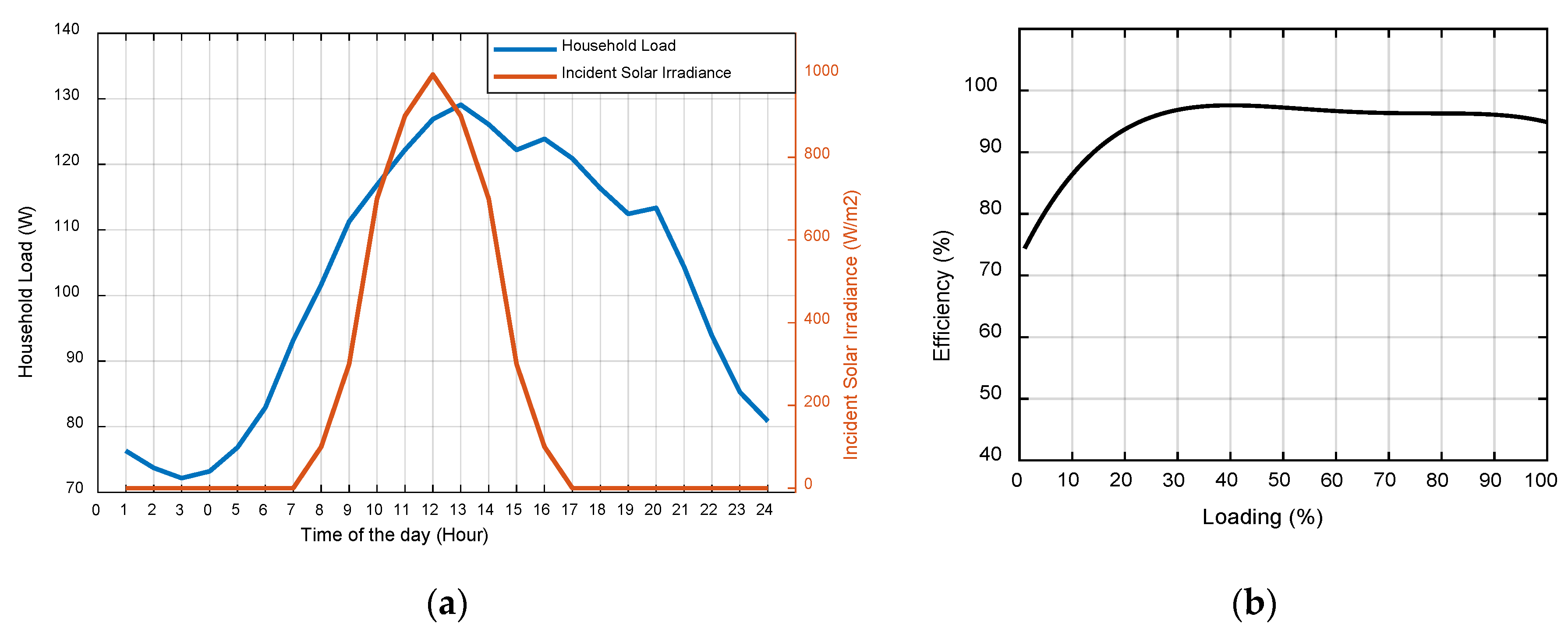
The power electronic conversion losses of the microgrid architecture depend upon the number of conversion stages encountered in the path of power flow from the source end to the load end. These converters mainly include a) an MPPT converter that is responsible for optimal PV integration and battery charging, b) a step-up converter for power distribution at a relatively higher voltage, and c) the load converter responsible for stepping down the voltage to the utilization level. The power electronic loss induced by each converter mainly consists of switching losses, conduction losses, and leakage losses [
28]. The conversion efficiency of power electronic converter can be modeled as a non-linear function of its output loading, as given by Equation (9) [
12,
28]:
where
PR is the rated power of the converter,
Po is the output power drawn from the converter at the given loading scenario, and
ki’s are the coefficients of energy conversion efficiency ranging from 0 to
K. In general, for the simplified analysis, higher-order terms are neglected, and
K is limited to the lower order, i.e.,
K = 2, which results in the simplification of Equation (9) in terms of Equation (10), as shown below [
27]:
However, simplification to lower-order coefficients may compromise the accuracy of analysis, and, therefore, higher-order coefficients need to be considered. Using the manufacturer’s datasheet parameters, a curve-fitting based method can be employed for the extraction of higher-order parameters of (9) for the accurate analysis of conversion efficiency and power electronic losses. The power electronic conversion losses incurred during
ith conversion stage
Pci can therefore be calculated using Equation (11):
3.3. Power Flow Diagrams and Village Scale PV Sizing Estimation
In order to estimate the total system power losses including conversion and distribution losses, it is necessary to visualize how power flows from the source end to the load end. Power flow diagrams presented below help to visualize the losses encountered in the path of power flow. Based on various components defined in the path of power flow, a compact formulation is formed for determining the operational efficiency of each architecture. Since the sizing of the system is directly dependent upon the system losses, power flow diagrams also give a fair idea of the system sizing calculation detailed in the sub-sections.
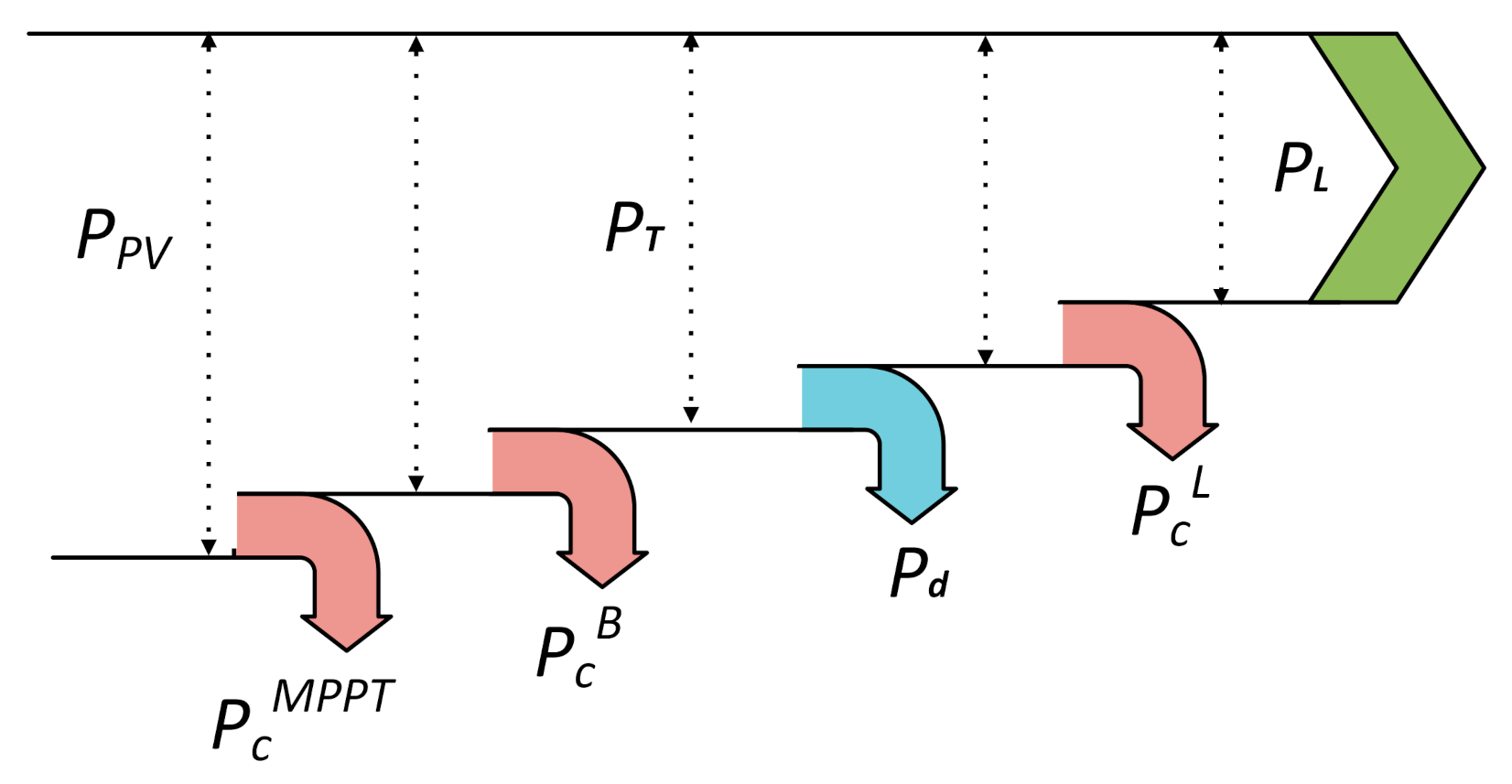
3.3.1. Power Flow Diagram and PV Sizing Estimation for CGCSA
The power flow diagram for CGCSA is shown in
Figure 5. From the architecture (presented in
Figure 1), it can be seen that the total power demanded by all the household loads
PL(
t) at any time
t is given by Equation (12):
The load power is fulfilled by the load converters installed at each household; therefore, based on output power loading and efficiency characteristics, input power needed at each household interface can be calculated using Equation (13):
where
PcL corresponds to the power electronic conversion losses across the household load converter and can be calculated using Equation (11) and load converter efficiency coefficients
kiL as given by Equation (14):
Once the power required at each household node is calculated, distribution losses across the distribution network can be found by scheduling the known amount of power at each household in Equation (3) and following the NR method modified for DC power flow, as mentioned above using Equations (4)–(8). Therefore, following the power flow diagram, the total power required at the input of distribution network
PT can be calculated using Equation (15):
Similarly, going across the power flow diagram and solving for boost converter losses
PCB and MPPT converter losses
PcMPPT using Equation (11) yields us the total power required from PV panel at any time t, as given by Equation (16).
If the incident irradiance in terms of average peak sun hours (PSH) is known for the location under consideration, this energy can be used for the calculation of PV panel sizing
SPV (
Wp) required to fulfill the given amount of load, as shown by Equation (17):
where
T is the total number of hours in a day, and
PPV(
t) is the total amount of time-varying power required for the load fulfillment. Therefore, when routing across the proposed power flow diagrams, not only the system losses but also the sizing of the system for a given architecture under consideration can be calculated.
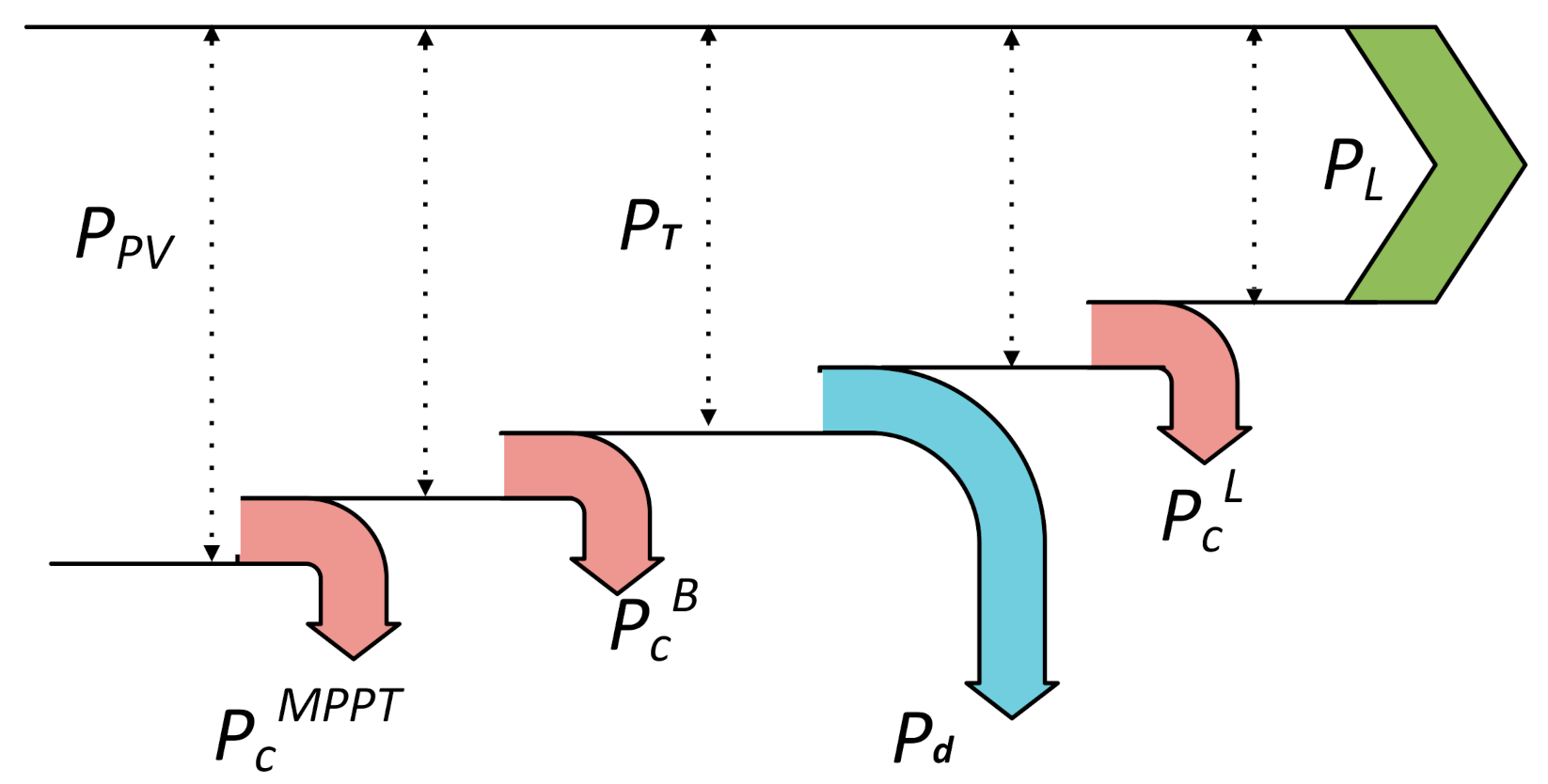
3.3.2. Power Flow Diagram and PV Sizing Estimation for CGDSA
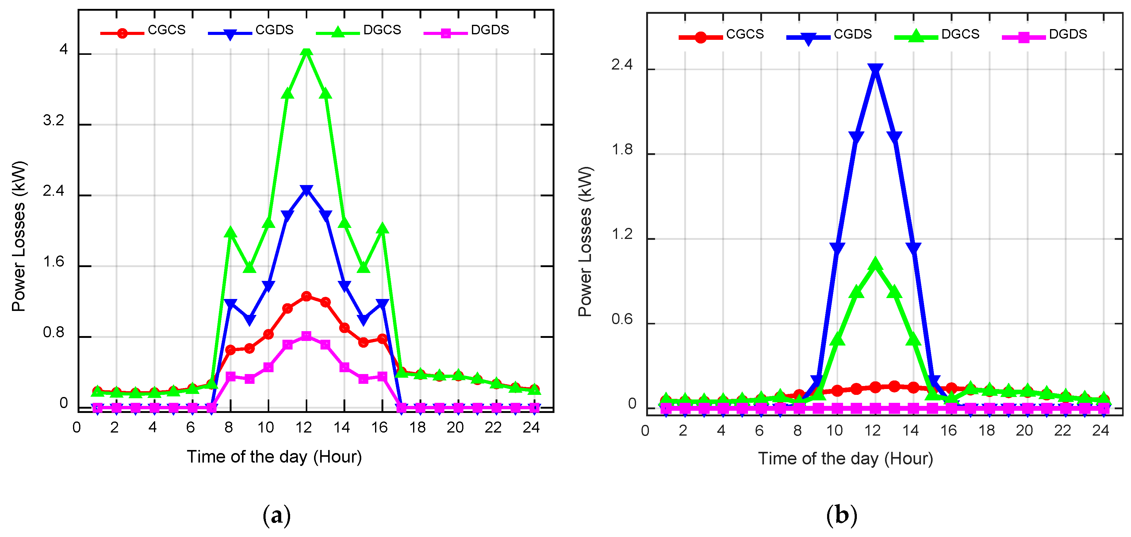
In the case of CGCSA, the generated power is stored locally and is distributed only when there is a load requirement; therefore, power distribution losses are independent of the incident irradiance and PV generation profile. On the contrary, in CGDSA, due to the unavailability of the local battery, all the generated power is distributed to household batteries in the duration of sun hours, when high irradiance is available. Since distribution losses increase in a quadratic fashion with the amount of power to be distributed, this architecture incurs higher distribution losses in PV generation hours. This quadratic increase in distribution losses is shown via a large length arrow in
Figure 6.
In order to estimate the PV sizing and system losses in CGDSA, the instantaneous power produced by PV panel
PPV(
t) needs to be represented in terms of its ambient conditions, including its cell temperature
Tc, ambient temperature
Tamb, incident irradiance
I (W/m
2), and temperature compensated incident irradiance
Itc (W/m
2), as given by Equation (18) [
25].
where
A is the area of the PV panels, and ηm is the module conversion efficiency. The temperature-compensated irradiance depends upon
I(
t) and
Tc and is given by Equation (19) [
39]:
The initial estimate of PV sizing is taken from total load demand at individual households, however, size is updated after each loss component, as shown in the power flow diagram. Therefore, losses across the load/battery converter
PcL are a function of run-time generated PV power and are processed by each household converter in terms of load converter efficiency coefficients
kiL, as given by Equation (21):
At this stage, distribution losses are calculated by scheduling power at each household and applying the NR method modified DC power flow as mentioned above. The overall distribution losses depend upon the amount of energy to be stored in each household and can be optimized using optimal charge/discharge algorithms based on each household requirements and forecasted load profile. However, in the current scope of the work, we assumed equal power storage at each household.
Similarly, power loss across the boost and the MPPT converters are also calculated using Equation (11), and overall PV sizing may be determined using Equation (23), as shown below:
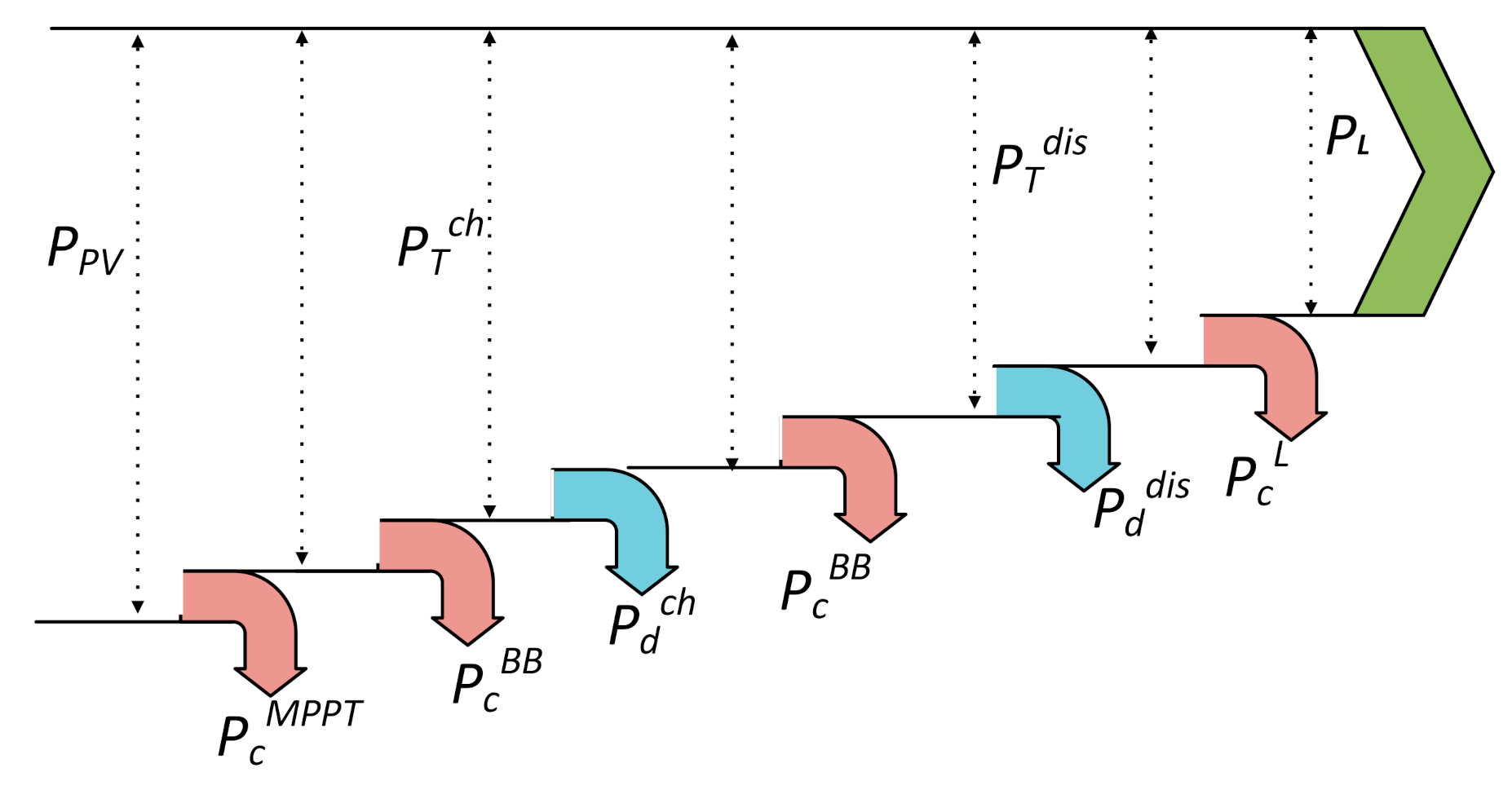
3.3.3. Power Flow Diagram and PV Sizing Estimation for DGCSA
In the case of DGCSA, part of the generated PV power is consumed locally by the household loads, while the remaining power is distributed to the central battery. Therefore, DGCSA has to encounter distribution losses during charging as well as discharging of the battery, as shown in
Figure 7. In order to estimate the overall system losses and PV sizing, charging and discharging instances of the battery need to be segregated. At any given instant of time
t, each household is either supplying power for battery charging, incurring charging distribution power loss
Pdch, or it is demanding power from the central battery, incurring discharging distribution power loss
Pddis. Therefore, if the power generation of the household is higher than its local demand, it aids in central battery charging, otherwise, it demands power, resulting in the discharge of the central battery.
The total power for the discharging stage
PTdis is calculated by the sum of individual discharging requirements by each household
PXdis(
t) as specified by Equations (24) and (25):
Here,
Pxdis can be used to calculate the distribution losses
Pddis during discharging state using the NR method modified for DC power flow using Equations (4)–(8). Similarly, the power for the charging stage
PTch(
t) can be calculated by the summation of charging contributions by the individual households
PXch(
t)
, as specified by using Equations (26) and (27):
Here,
Pxch can be used to calculate the distribution losses
Pdch during the charging state using the NR method modified for DC power flow as defined above. The converter losses, including MPPT conversion losses for each converter
PcMPPT, buck-boost converter losses
PcBB, and load converter losses
PcL, can be evaluated using Equation (11) as discussed in the above architectures. Following the diagram of power flow, village-scale PV sizing for DGCSA can be calculated using Equation (28):
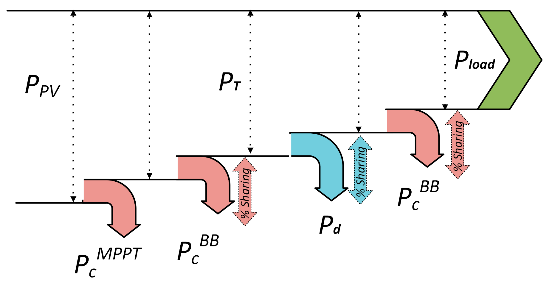
3.3.4. Power Flow Diagram and PV Sizing Estimation for DGCSA
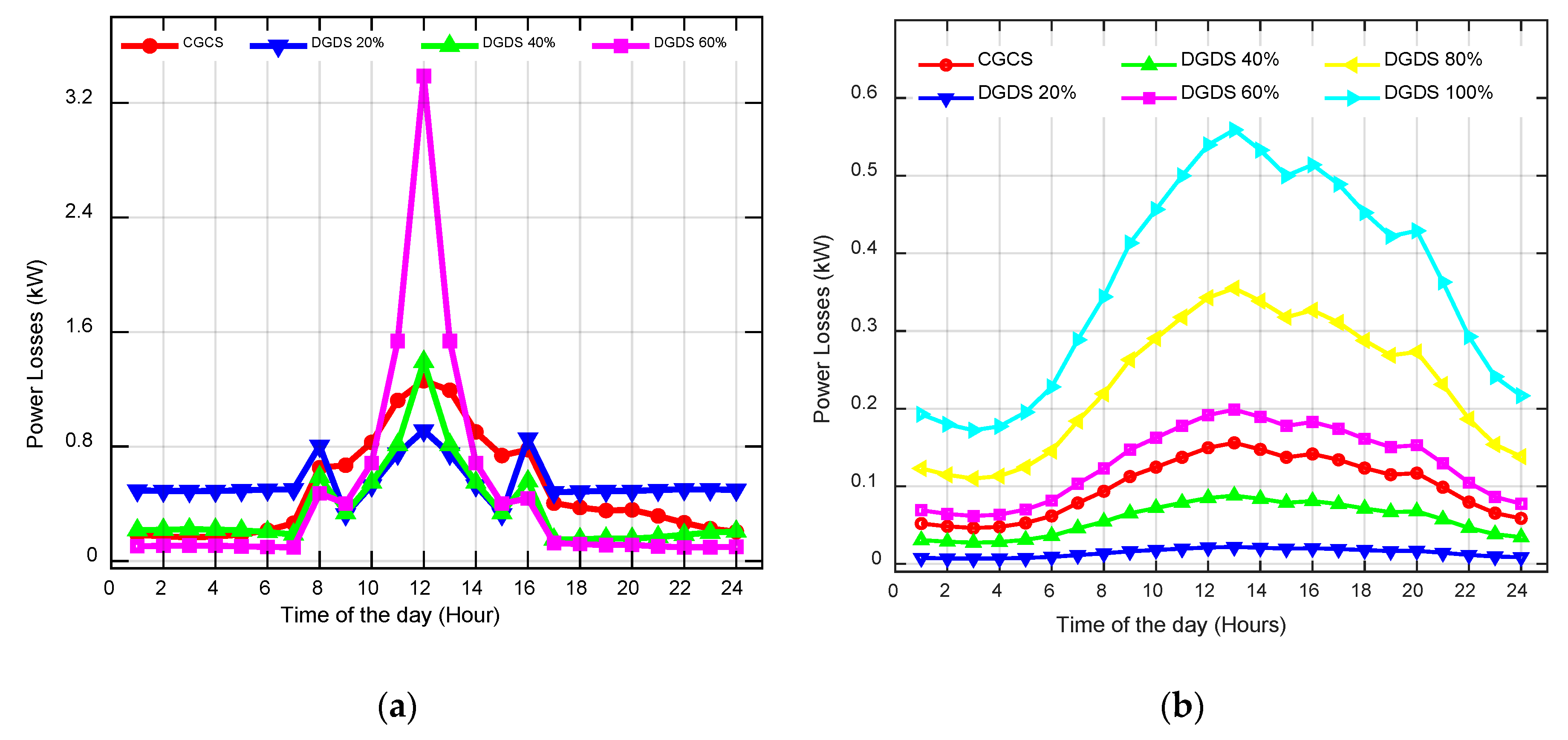
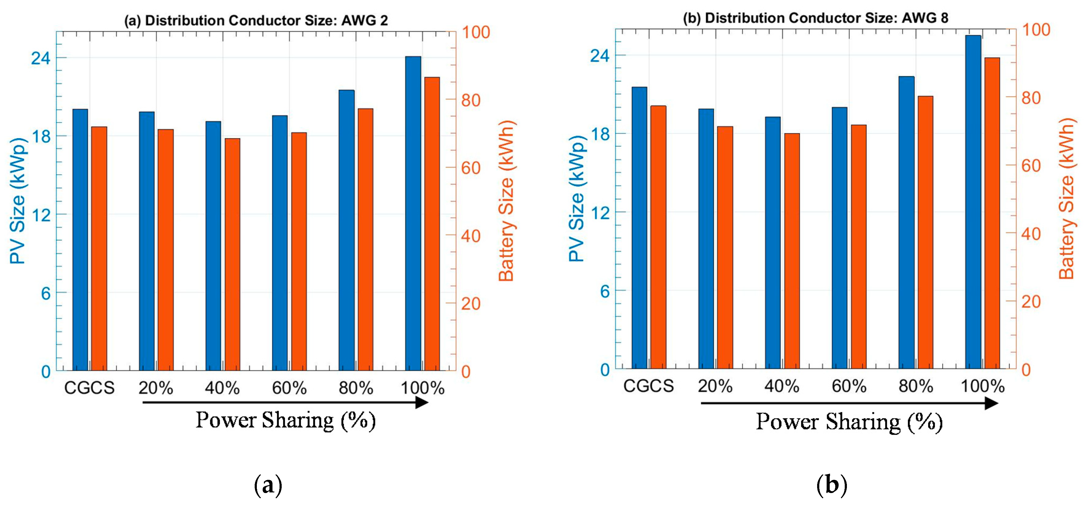
In the case of DGDSA, if every household is self-sufficient, i.e., it can fulfill its household load demand using indigenous PV generation and battery resources, distribution losses become zero, and only converter losses incur in the path of power flow from the source end to the load end. However, as described earlier, DGDSA may have the capability to share power among the neighboring households, therefore, distribution losses become a function of power-sharing among households. With the percentage increase in power-sharing, distribution losses increase as shown in
Figure 8 below. Not only the distribution losses but also the converter losses become a function of power-sharing among households as shown by the power flow diagram of DGDSA.
Firstly considering the scenario where every household is self-sufficient, the load demand is fulfilled by either the PV generation or the battery storage. Since battery voltage is kept the same as load voltage, all the generated power is processed through the common battery/load bus as shown in
Figure 4. The MPPT converter losses become
PcMPPT becomes a function of incident irradiance and ambient conditions as explained by Equations (18)–(20), and overall village scale size can be determined using a simple relationship defined by Equation (29):
However, with the increase in power-sharing among neighboring households, distribution and conversion losses become evident and need to be calculated for the overall PV size determination. Therefore, following the power flow diagram, if any of the houses are not operating in self-sufficient mode, either supply power or demand power from the DC bus link through, which is connected with the neighboring households. In either case, distribution losses may be calculated using the information of power processed by buck-boost converters and distribution losses. For a given percentage of power-sharing
S, the conversion losses across the buck-boost converter at the distribution interface of the supplying and receiving household can be determined using Equation (30):
The distribution losses
Pd across the power-sharing network can be calculated using the scheduled load power matrix in terms of power-sharing coefficient
S and load demand at each household
PX’, as defined by Equation (31), and applying the procedure defined by Equations (4)–(8):
where positive
S corresponds to the power supplying household in the network, and negative
S corresponds to the power-consuming household. Once conversion and distribution losses are determined, the overall village-level PV sizing can be determined using Equation (32):
3.4. Village Scale Battery Sizing
Since power generation from solar PV is intermittent and subject to variation in weather and ambient conditions of temperature and incident irradiance, therefore, the battery storage system not only provides the buffer for variations but also provides power during the non-available sun hours. In order to calculate the size of the battery, various parameters including battery technology (lead-acid, Li-ion, Ni-Cd, etc.), price, energy and volume density, and life cycle considerations are taken into account. Moreover, battery efficiency and depth of discharge are other key parameters that need to be considered for practical implementations [
40]. Limiting the depth of discharge to higher values generally enhances the lifetime of the battery as well as reduces the maintenance cost [
40]. Taking all these factors into consideration and the availability of the village scale PV size, a first-order cost calculation model is determined for the village-scale battery sizing
SB (Wh). It should be mentioned that, once the solar PV size is determined, the battery sizing is independent of the architecture, and the first-order cost model presented by (33) is valid for all the architectures under consideration. The battery system must be capable of storing and supplying the total energy when the sun is not available. Along with that, it must also store extra energy dissipated during the charge/discharge cycle. Moreover, to extend the battery life, batteries are generally oversized such that there is a limit on minimum discharging state
(%). The overall battery sizing for each of the architecture is given by Equation (33) [
35]:
where
ηB is the battery charge–discharge cycle efficiency,
T is the total number of hours in the day, PSH is the estimated average peak sunlight hours, and
PPV(
t) is the time-varying power required to fulfill the load as determined in the above sections.
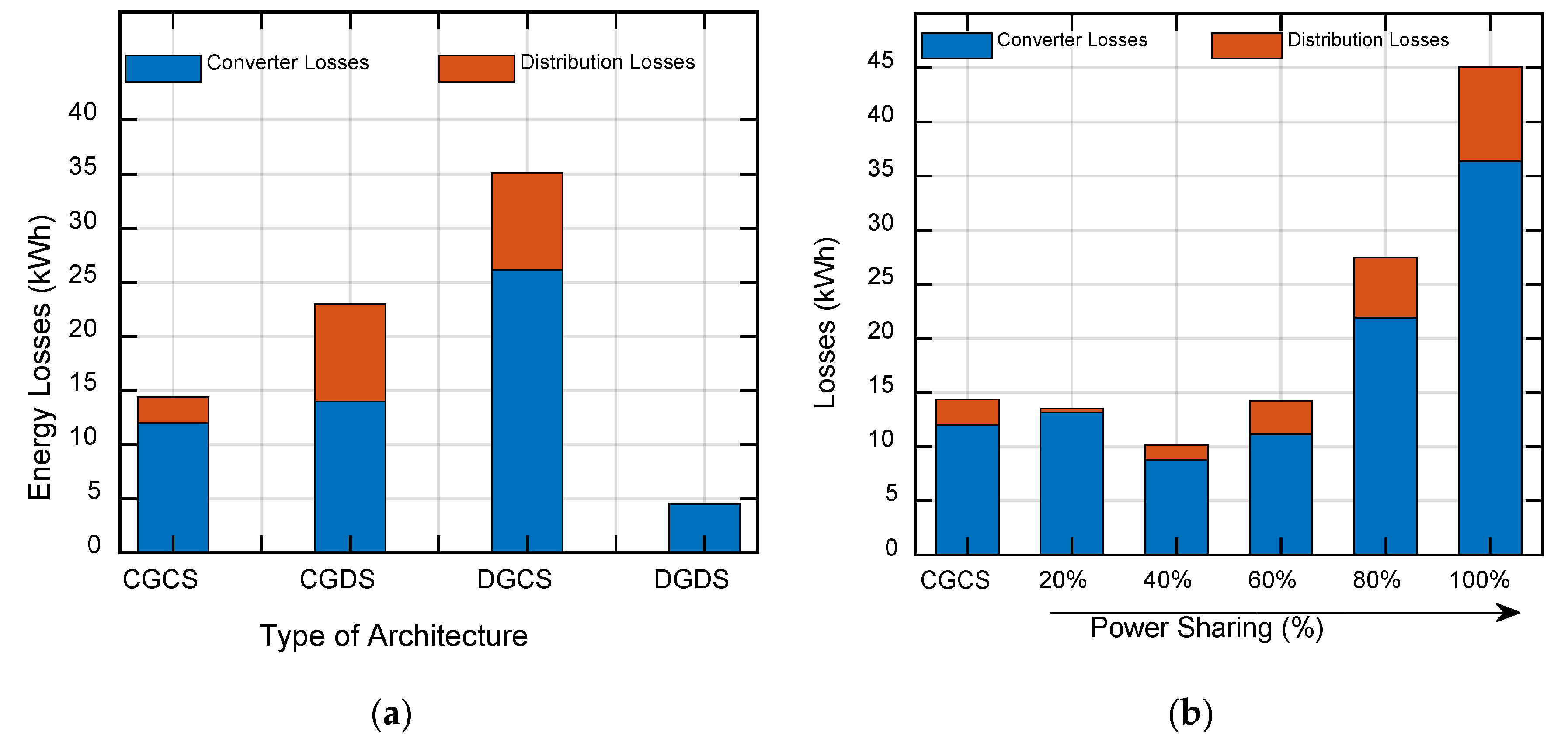
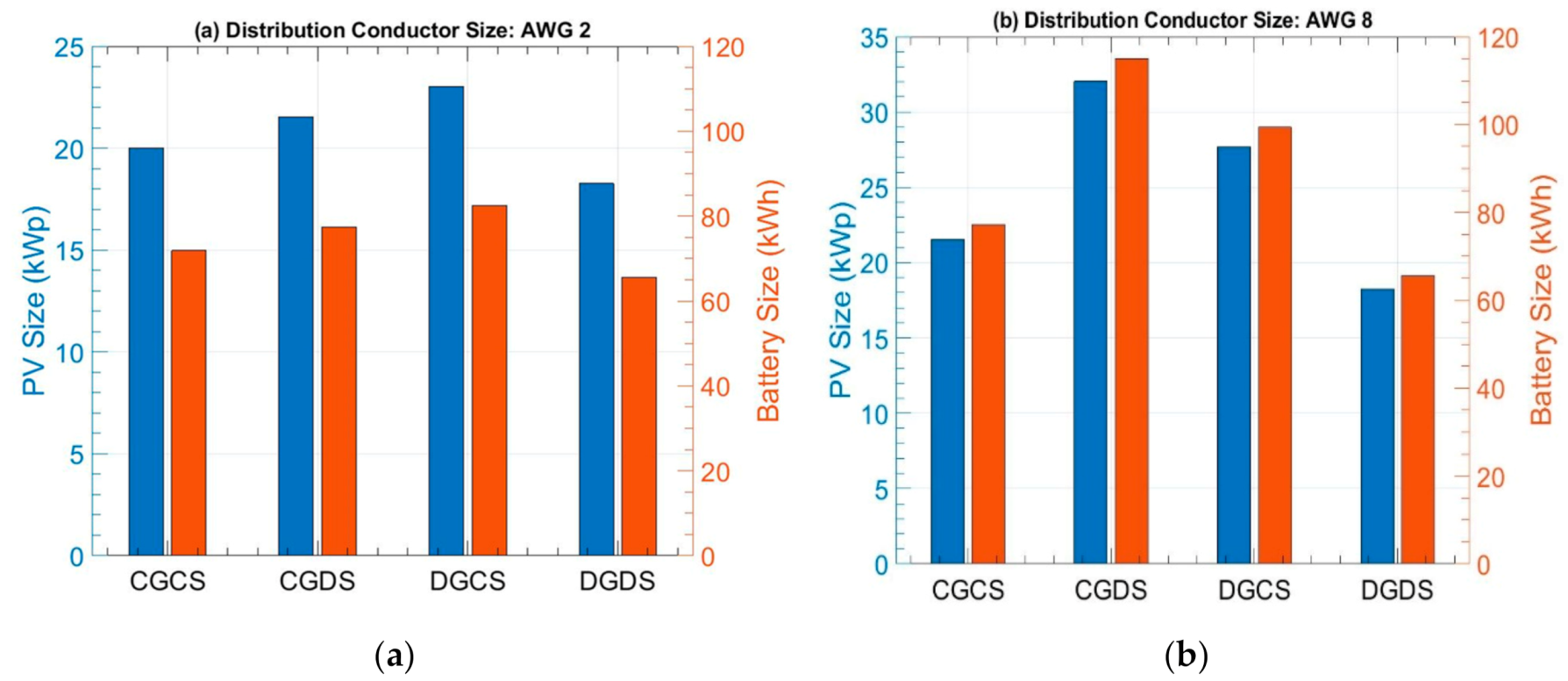
6. Conclusions
A detailed comparative analysis of various PV-based DC microgrid architectures for rural electrification applications is presented in this work. Along with the details of architecture, a mathematical framework for the evaluation of losses and system sizing is also presented. Various parameters that affect system losses and sizing are identified, and architecture’s efficiencies are evaluated accordingly. In all operation scenarios, DGDSA and CGCSA outperform the other two architectures, i.e., CGDSA and DGCSA. Although CGCSA is simple to control and implement, it has been shown that, for villages with lower usage diversity and minimal power-sharing requirements, DGDSA can be the optimal choice concerning system losses and system sizing. However, with the increase in usage diversity and power-sharing requirements, not only do the control and the complexity enhance but the system losses and sizing requirements enhance as well. In such scenarios, CGCSA can be the optimal choice for system designers. Different power-sharing levels can be evaluated using the proposed framework; therefore, optimal resource utilization can be achieved. Moreover, DGDSA offers enhanced functionalities, including the capability of bidirectional energy transaction and power pooling for community applications. Therefore, it is the choice of the designer and the specifications of the subscriber as to which architecture is preferred, however, the framework presented is generic in nature and gives complete insight into loss analysis and sizing calculation for all possible architectures. The proposed model can be used by system planners for efficiency analysis, system sizing, and architecture selection. Moreover, the proposed model and the associated analysis can be extended to evaluate the additional losses, e.g., partial shading effects and battery charging/discharging losses along with their dependence on the architecture under consideration. The proposed sizing framework can also be extended for upfront cost analysis, and results may be validated using standard renewable energy planning software, e.g., Hybrid Optimization Model for Multiple Energy Resources (HOMER) in future work. Researchers can also extend this model for developing an optimal peer-to-peer power-sharing framework in rural microgrids. The introduction of proper-sized centralized storage could improve performances of the DGDSA by mitigating the complexity of the system control and by optimizing the power-sharing requirements. Therefore, this work may also pave ways for the development of hybrid architectures, e.g., distributed generation architecture with mixed (distributed and centralized) storage for efficient rural electrification implementations in the future.


