
Assessment of the Impact of Coal Mining on Water Resources in Middelburg, Mpumalanga Province, South Africa: Using Different Water Quality Indices


Abstract
1. Introduction
- To use existing water quality monitoring data for both surface water and groundwater sampling points in the Middelburg region and compare it with the water quality resource objectives of the study area;
- To use different water quality indices (CCME–WQI and CPI) in combination with the water quality guidelines to determine the impacts of coal mining activities on surface water and groundwater quality around the study area;
- To evaluate the interrelationship trends of the surface water and groundwater quality data;
- To provide possible and efficient mitigation measures for the protection of water resources from coal mining and other related land-use activities.
2. Materials and Methods
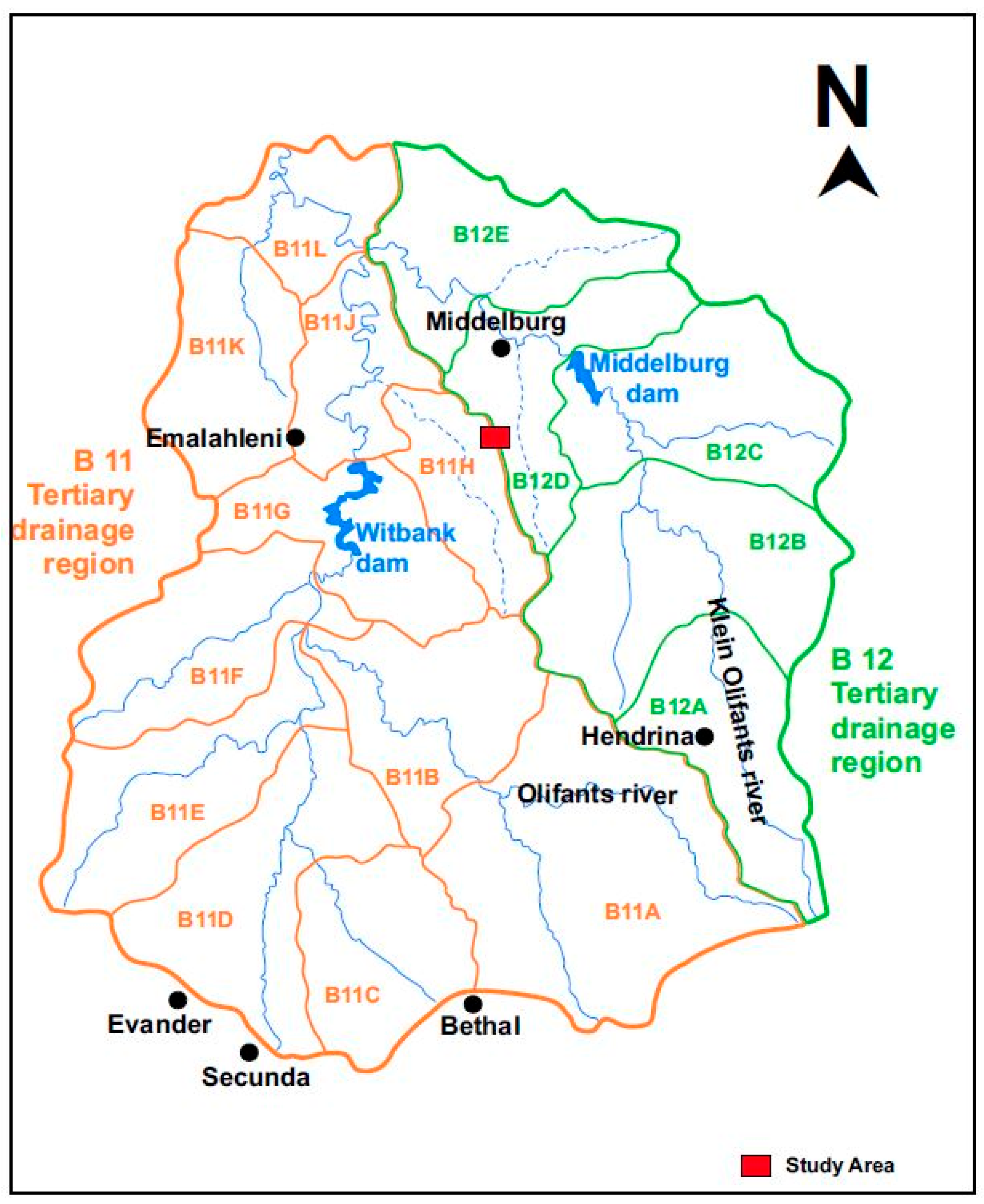
2.1. Description of Study Area
2.2. Field Sampling and Analysis
2.3. Surface Water
2.4. Groundwater
2.5. Selection of Sampling Sites
2.6. Data Analysis
2.6.1. Water Quality Analysis
2.6.2. Water Pollution Indices
- F1 (scope) represents the number of variables whose objectives were not met.
- PI represents pollution index of individual parameters.
- N is the number of parameters.
- Ci is the measured concentration of ith paramete
- Si is the standard value of ith parameter.
2.6.3. Statistical Analysis
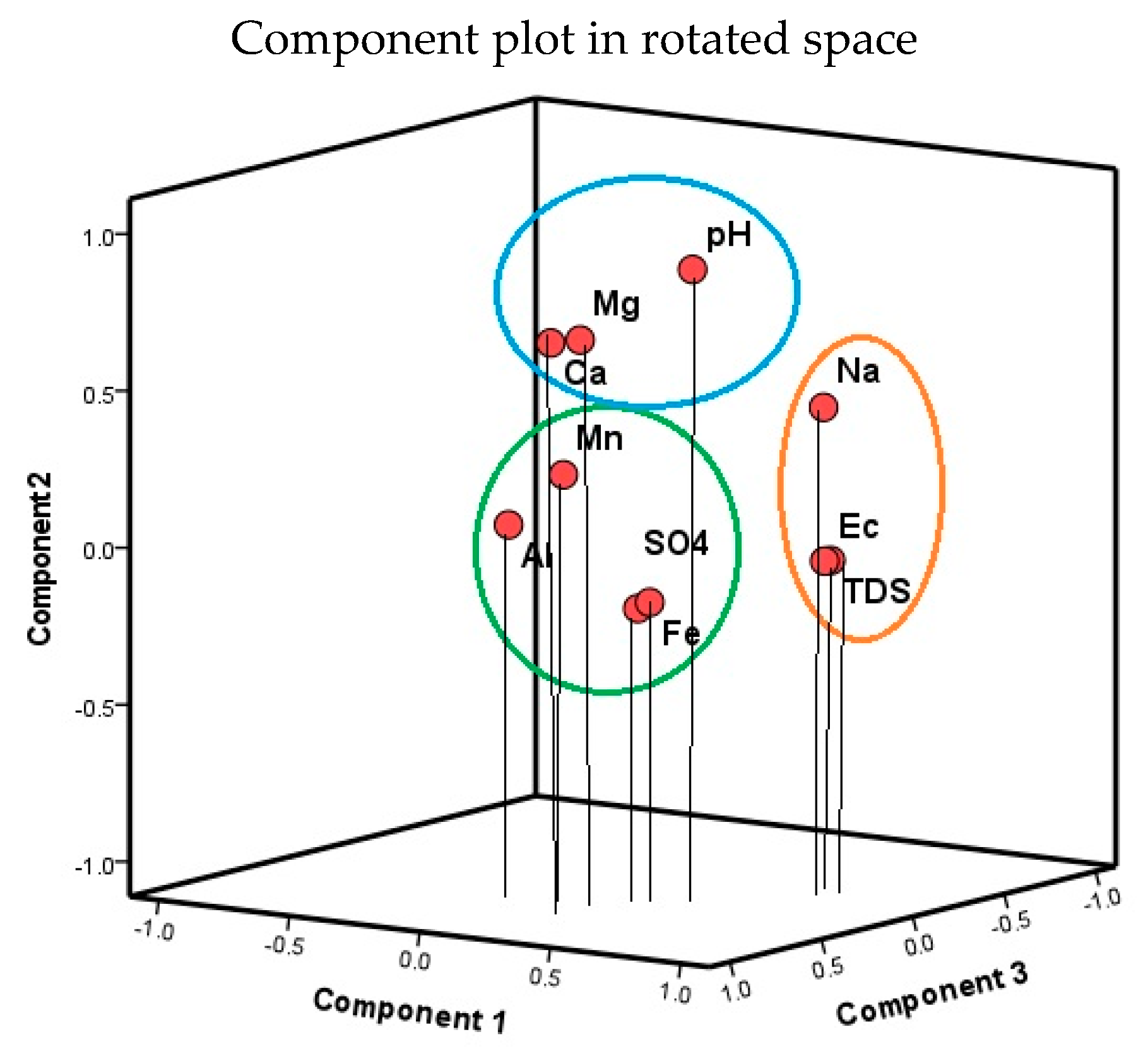
2.6.4. Principal Component Analysis
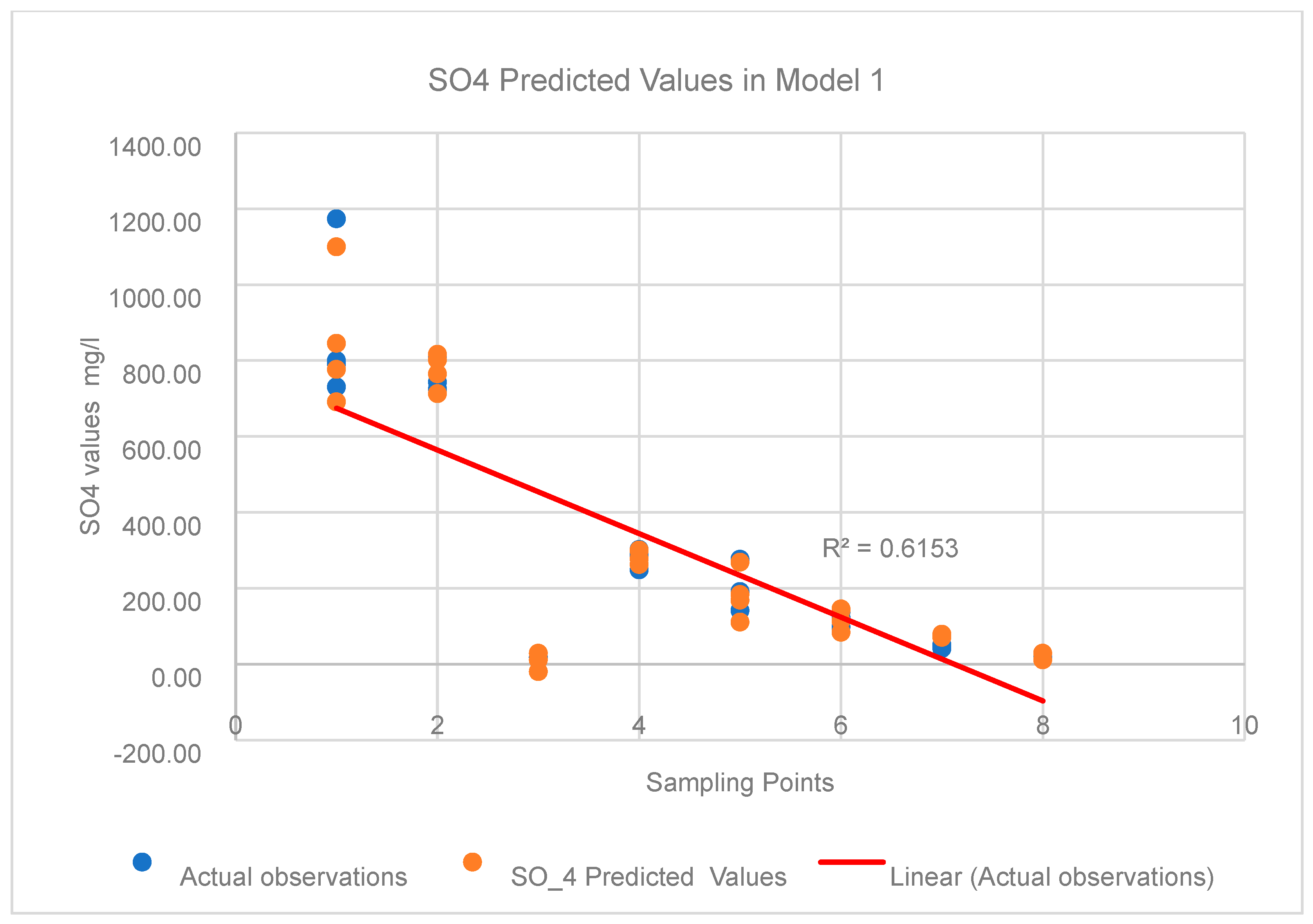
2.6.5. Multiple Linear Regression
- represents the dependent variable.
- represents several independent variables.
- represents the regression coefficient.
- represents the random error.
- is the regression sum of squares.
- is the observed variance.
- is sum of squares of the residuals.
3. Results
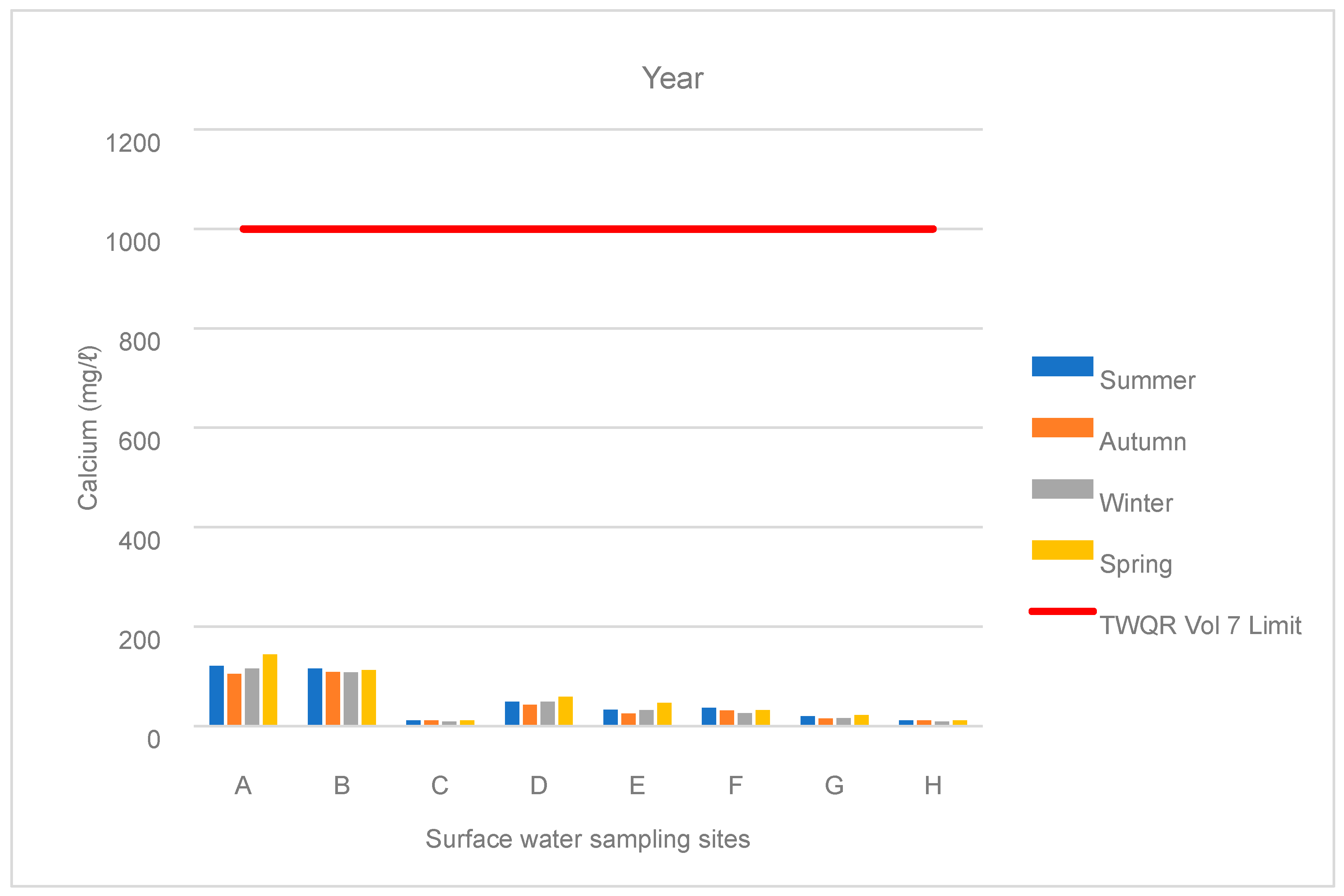
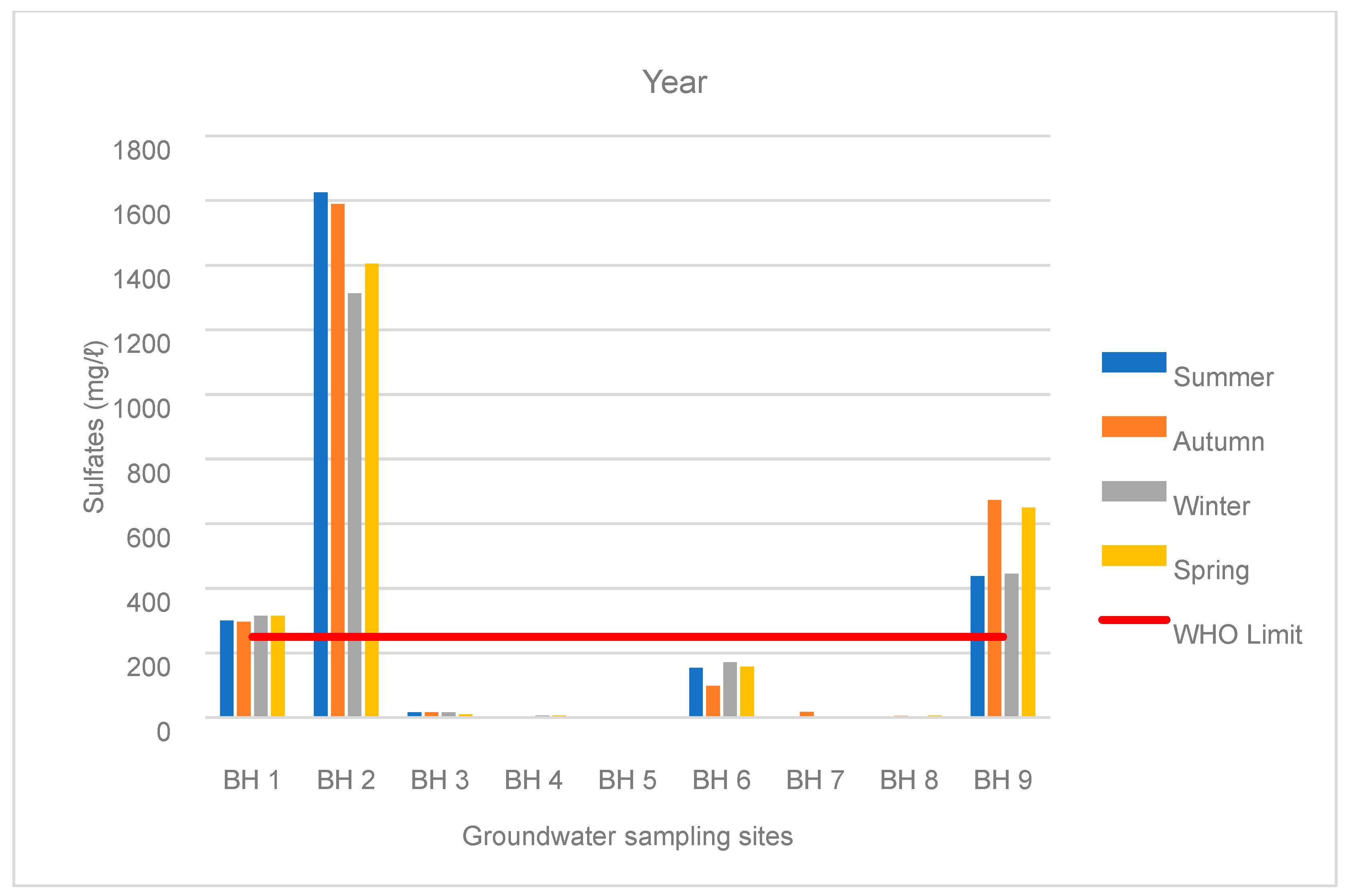
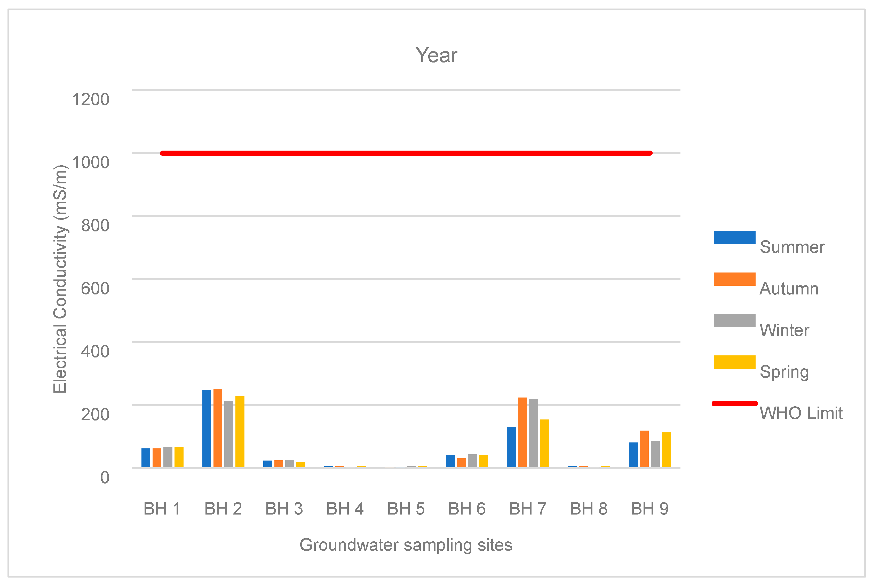
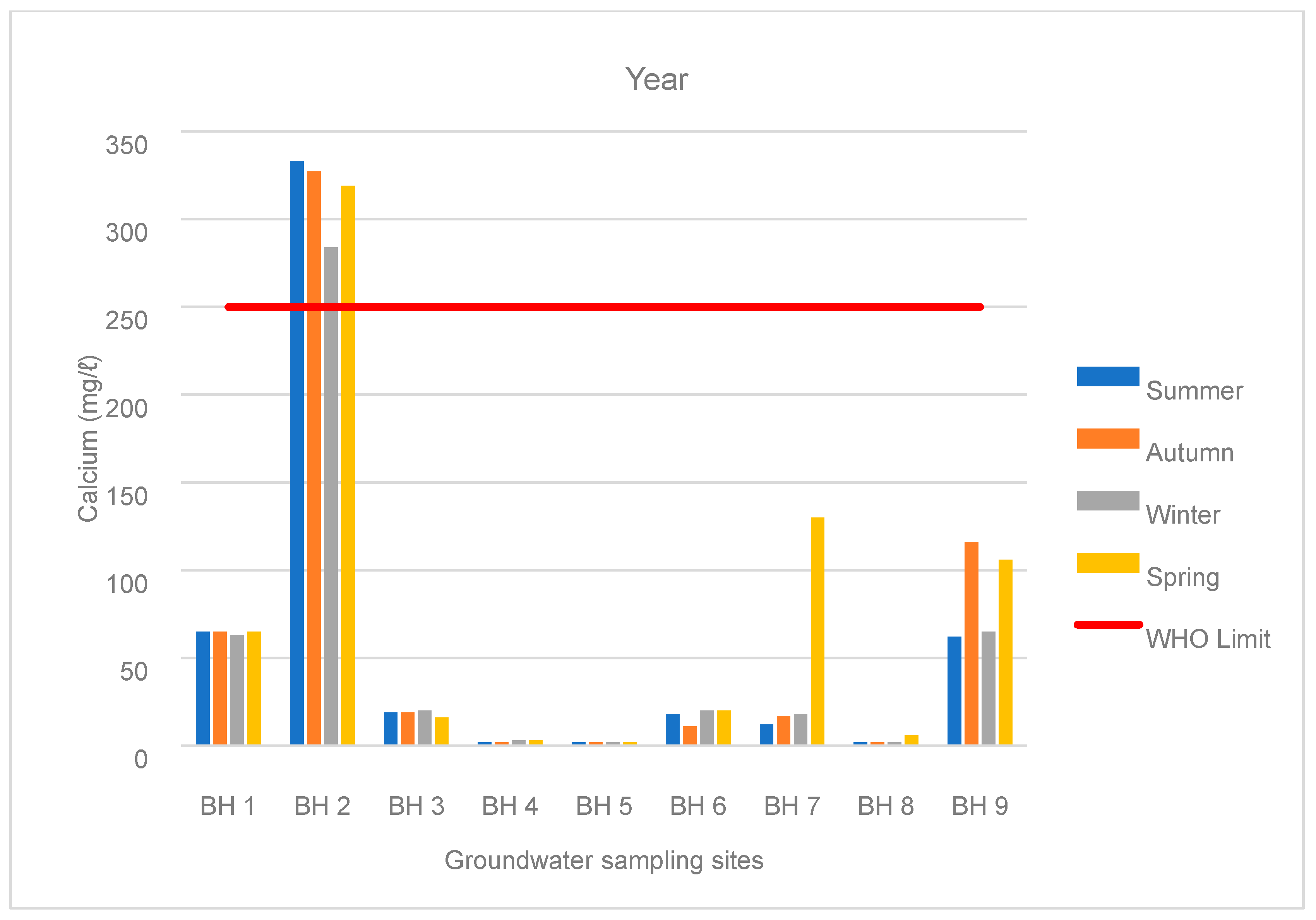
3.1. Water Chemistry
3.2. Canadian Council of Ministers of the Environment Water Quality Index
3.3. Comprehensive Pollution Index
3.4. Comparison between the Two Indices
3.4.1. Multivariate Statistical Analysis Results
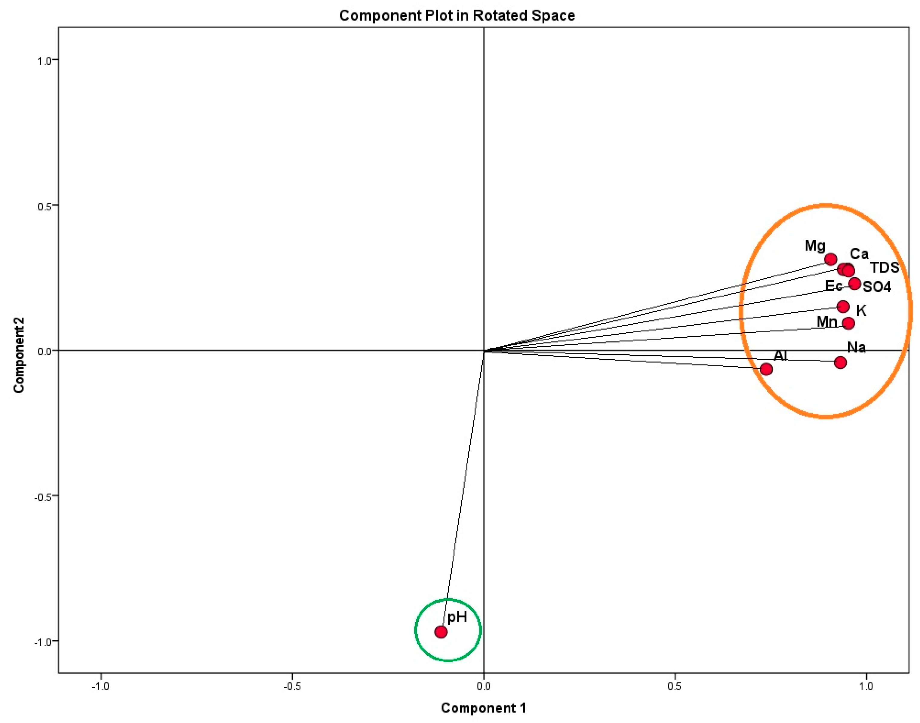
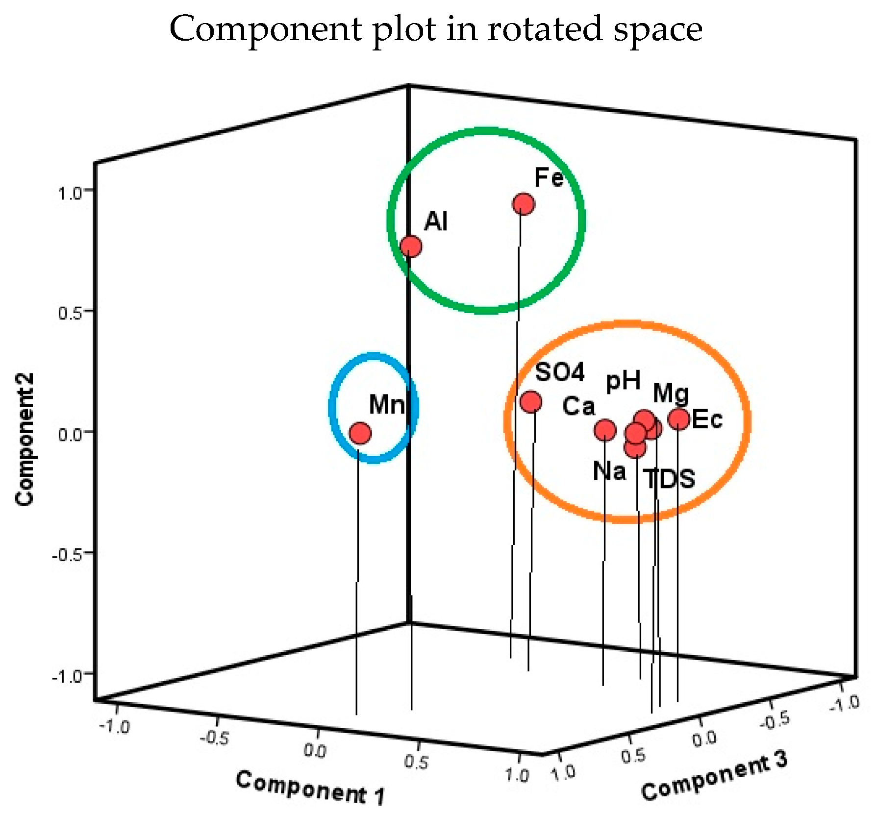
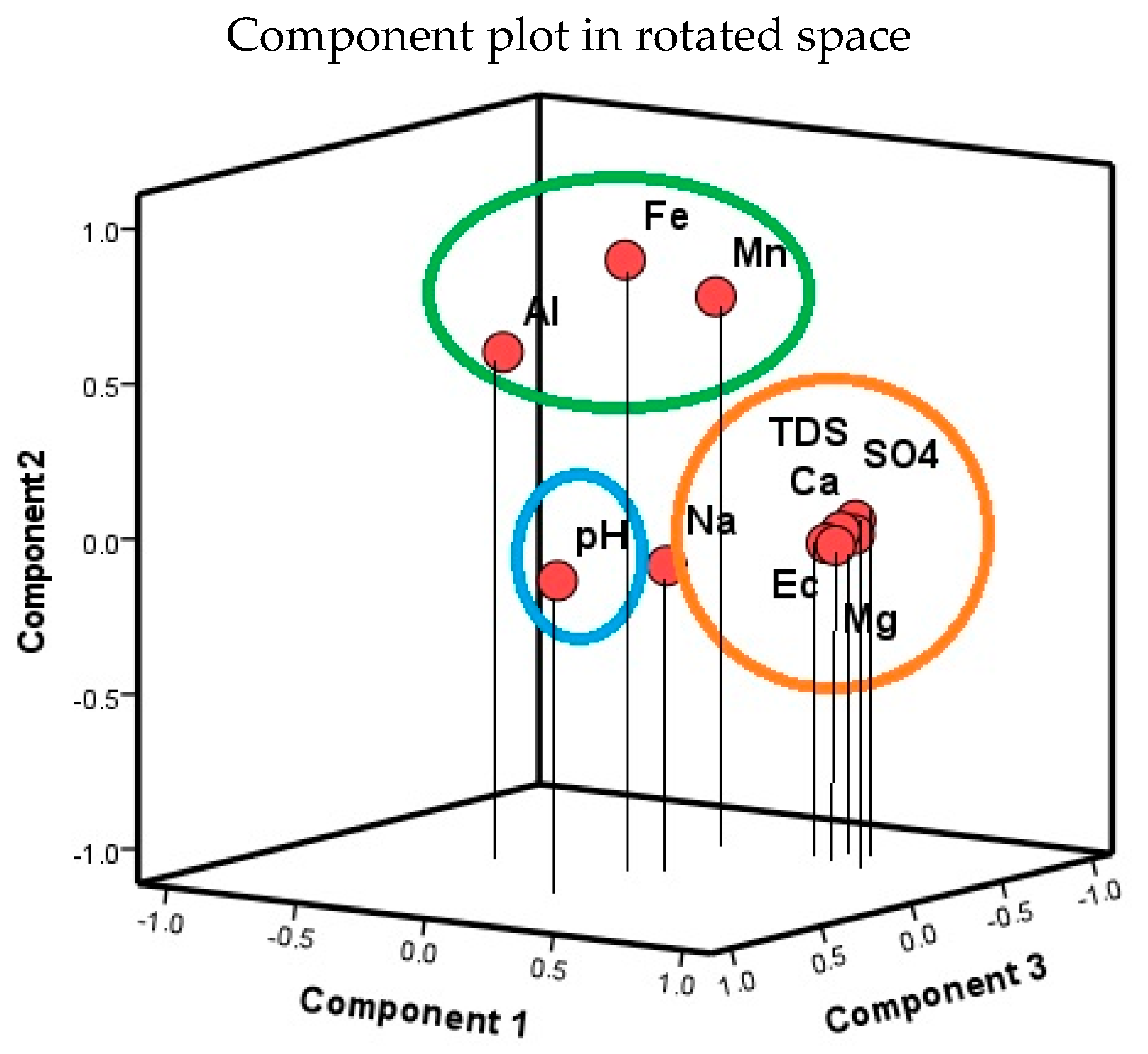
Principal Component Analysis
Linear Regression Analysis
4. Discussion
5. Conclusions and Recommendations
Author Contributions
Funding
Data Availability Statement
Acknowledgments
Conflicts of Interest
Ethical Approval
References
- Eberhard, A. The Future of South African Coal: Market, Investment, and Policy Challenges; Working Paper 100; Program on Energy and Sustainable Development; Freeman Spogli Institute for International Studies; Stanford University: Stanford, CA, USA, 2011; Available online: https://fsi9-prod.s3.us-west-1.amazonaws.com/s3fs-public/WP_100_Eberhard_Future_of_South_African_Coal.pdf (accessed on 22 July 2024).
- Makgae, M. The Status and Implications of the AMD Legacy Facing South Africa. In Proceedings of the International Mine Water Association Annual Conference, Bunbury, Australia, 29 September–4 October 2012; pp. 327–334. Available online: http://mwen.info/docs/imwa_2012/IMWA2012_Makgae_327.pdf (accessed on 22 July 2024).
- Oelofse, S.H.H.; Hobbs, P.J.; Rascher, J.; Cobbing, J.E. The Pollution and Destruction Threat of Gold Mining Waste on the Witwatersrand—A West Rand Case Study. In Proceedings of the 10th International Symposium on Environmental Issues and Waste Management in Energy and Mineral Production (SWEMP 2007), Bangkok, Thailand, 11–13 December 2007; pp. 617–627. Available online: https://www.anthonyturton.com/assets/my_documents/my_files/983_SWEMP.pdf (accessed on 22 July 2024).
- Romer, C.D. What ended the great depression? J. Econ. Hist. 1992, 52, 757–784. Available online: https://www.jstor.org/stable/2123226 (accessed on 22 July 2024). [CrossRef]
- Grande, J.A.; Borrego, J.; Morales, J.A.; De la Torre, M.L. A description of how metal pollution occurs in the Tinto–Odiel rias (Huelva–Spain) through the application of cluster analysis. Mar. Pollut. Bull. 2003, 46, 475–480. [Google Scholar] [CrossRef]
- Shang, Y.; Qi, P. Study on environmental negative effect and control of waste coal mine. Coal Eng. 2018, 50, 147–150. (In Chinese) [Google Scholar]
- Ashton, P.J.; Harwick, D.; Breen, C.M. Changes in water availability and demand within South Africa’s shared river basins as determinants of regional social ecological resilience. In Exploring Sustainability Science: A South African Perspective; Burns, M.J., Weaver, A., Clark, W., Kates, R., Eds.; African Sun Media: Stellenbosch, South Africa, 2008; pp. 279–310. [Google Scholar]
- Oberholster, P.J.; Botha, A.-M.; Cloete, T.E. Biological and chemical evaluation of sewage water pollution in the Rietvlei nature reserve wetland area, South Africa. Environ. Pollut. 2008, 156, 184–192. [Google Scholar] [CrossRef]
- Quibell, G.; Van Vliet, H.; Van der Merwe, W. Characterizing cause-and effect relationships in support of catchment water quality management. Water SA 1997, 23, 193–199. Available online: https://www.wrc.org.za/wp-content/uploads/mdocs/WaterSA_1997_03_1021.PDF (accessed on 22 July 2024).
- Uddin, M.G.; Nash, S.; Olbert, A.I. A review of water quality index models and their use for assessing surface water quality. Ecol. Indic. 2021, 122, 107218. [Google Scholar] [CrossRef]
- Kachroud, M.; Trolard, F.; Kefi, M.; Jebari, S.; Bourrié, G. Water quality indices: Challenges and application limits in the literature. Water 2019, 11, 361. [Google Scholar] [CrossRef]
- Tirkey, P.; Bhattacharya, T.; Chakraborty, S. Water quality indices: Important tools for water quality assessment: A review. Int. J. Adv. Chem. 2013, 1, 15–28. Available online: https://airccse.com/ijac/papers/1115ijac02.pdf (accessed on 22 July 2024).
- Son, C.T.; Giang, N.T.H.; Thao, T.P.; Nui, N.H.; Lam, N.T.; Cong, V.H. Assessment of Cau River water quality assessment using a combination of water quality and pollution indices. J. Water Supply Res. Technol.—AQUA 2020, 69, 160–172. [Google Scholar] [CrossRef]
- Finotti, A.R.; Finkler, R.; Susin, N.; Schneider, V.E. Use of water quality index as a tool for urban water resources management. Int. J. Sustain. Dev. 2015, 10, 781–794. [Google Scholar] [CrossRef]
- Oberholster, P.F.; Goldin, J.; Xu, Y.; Kanyerere, T.; Oberholster, P.J.; Botha, A.-M. Assessing the adverse effects of a mixture of AMD and sewage effluent on a sub-tropical dam situated in a nature conservation area using a modified pollution index. Int. J. Environ. Res. 2021, 15, 321–333. [Google Scholar] [CrossRef]
- Tang, T.; Zhai, Y.; Huang, K. Water Quality Analysis and Recommendations through Comprehensive Pollution Index Method. J. Manag. Sci. Eng. 2011, 5, 95–100. [Google Scholar] [CrossRef]
- Matta, G.; Kumar, A.; Uniyal, D.P.; Singh, P.; Kumar, A.; Dhingra, G.K.; Kumar, A.; Naik, P.K.; Shrivastva, N.G. Temporal assessment using WQI of River Henwal, a tributary of river Ganga in Himalayan region. Int. J. Env. Rehab. Conserv. 2017, VIII, 187–204. Available online: https://essence-journal.com/wp-content/uploads/Volume_VIII/Issue_1/Temporal-assessment-using-WQI-of-River-Henwal-a-Tributary-of-River-Ganga-in-Himalayan-Region.pdf (accessed on 22 July 2024).
- Mishra, S.; Sharma, M.P.; Kumar, A. Assessment of surface water quality in Surha Lake using pollution index, India. J. Matr. Environ. Sci. 2016, 7, 713–719. Available online: https://jmaterenvironsci.com/Document/vol7/vol7_N3/84-JMES-1858-2015-Mishra.pdf (accessed on 22 July 2024).
- Lumb, A.; Halliwell, D.; Sharma, T. Application of CCME water quality index to monitor water quality: A case of the Mackenzie River Basin, Canada. Environ. Monit. Assess. 2006, 113, 411–429. [Google Scholar] [CrossRef] [PubMed]
- Espejo, L.; Kretschmer, N.; Oyarzún, J.; Meza, F.; Núñez, J.; Maturana, H.; Soto, G.; Oyarzo, P.; Garrido, M.; Suckel, F.; et al. Application of water quality indices and analysis of the surface water quality monitoring network in semiarid North-Central Chile. Environ. Monit. Assess. 2012, 184, 5571–5588. [Google Scholar] [CrossRef] [PubMed]
- Islam, M.M.; Karim, R.; Zheng, X.; Li, X. Heavy metal and metalloid pollution of soil, water and foods in Bangladesh: A critical review. Int. J. Environ. Res. Public Health 2018, 15, 2825. [Google Scholar] [CrossRef] [PubMed]
- Uddin, M.G.; Moniruzzaman, M.; Khan, M. Evaluation of groundwater quality using CCME water quality index in the Rooppur nuclear power plant area, Ishwardi, Pabna, Bangladesh. Am. J. Environ. Prot. 2017, 5, 33–43. [Google Scholar] [CrossRef]
- Karim, M.; Das, S.K.; Paul, S.C.; Islam, M.F.; Hossain, S. Water quality assessment of Karrnaphuli River, Bangladesh using multivariate analysis and pollution indices. AJEE 2018, 7, 1–11. [Google Scholar] [CrossRef]
- McCarthy, T.S. The impact of acid mine drainage in South Africa. S. Afr. J. Sci. 2011, 107, 1–7. [Google Scholar] [CrossRef]
- Department of Water Affairs and Forestry. Olifants Water Management Area: Internal Strategic Perspective; Report P WMA 04/0000/00/0304; Department of Water Affairs and Forestry: Pretoria, South Africa, 2004. Available online: https://www.dws.gov.za/Documents/Other/WMA/Olifants_ISP.pdf (accessed on 22 July 2024).
- Adler, R.; Rascher, J. A Strategy for the Management of Acid Mine Drainage from Gold Mines in Gauteng; Report no. CSIR/NRE/PW/ER/2007/0053/C; Council for Scientific and Industrial Research: Pretoria, South Africa, 2007. [Google Scholar]
- Pulles, W.; Banister, S.; Van Biljon, M. The Development of Appropriate Procedures towards and after Closure of Underground Gold Mines from a Water Management Perspective; Report 1215/1/05; Water Research Commission: Pretoria, South Africa, 2005; Available online: https://www.wrc.org.za/wp-content/uploads/mdocs/1215-1-051.pdf (accessed on 22 July 2024).
- Atangana, E. An indices-based water quality model to evaluate surface water quality: A case study in Vaalwaterspruit, Mpumalanga, South Africa. J. Afr. Earth Sci. 2023, 205, 105001. [Google Scholar] [CrossRef]
- Midgley, D.C.; Pitman, W.V.; Middleton, B.J. Surface Water Resources of South Africa; WRC Report No 298/1.1/94; Water Research Commission: Pretoria, South Africa, 1990; Volume 1. [Google Scholar]
- Cairncross, B.; McCarthy, T.S. A geological investigation of Klippan in Mpumalanga province, South Africa. S. Afr. J. Geol. 2008, 111, 421–428. [Google Scholar] [CrossRef]
- Wilson, M.G.C.; Anhaeusser, C.R. The Mineral Resources of South Africa, 6th ed.; Handbook 16; Council for Geoscience: Pretoria, South Africa, 1998. [Google Scholar]
- Visser, J.N.J. The permo-carboniferous Dwyka Formation of Southern Africa: Deposition by a predominantly subpolar marine ice sheet. Palaeogeogr. Palaeoclimatol. Palaeoecol. 1989, 70, 377–391. [Google Scholar] [CrossRef]
- Department of Water and Sanitation, South Africa. National Water Act, 1998 (Act No. 36 of 1998): Classes and 25 Resource Quality Objectives of Water Resources for the Olifants Catchment; Government Gazette No. 466; Department of Water and Sanitation, South Africa: Pretoria, South Africa, 2016. Available online: https://www.gov.za/sites/default/files/gcis_document/201604/39943gon466.pdf (accessed on 22 July 2024).
- Heaton, J. Secondary analysis of qualitative data: An overview. Hist. Soc. Res. 2008, 33, 33–45. Available online: https://www.jstor.org/stable/20762299 (accessed on 22 July 2024).
- Smith, E. Pitfalls and Promises: The Use of Secondary Data Analysis in Educational Research; McGraw-Hill Education: New York, NY, USA, 2008. [Google Scholar]
- Department of Water Affairs and Forestry. Best Practice Guideline G3: Water Monitoring Systems; Department of Water Affairs and Forestry: Pretoria, South Africa, 2006. Available online: https://www.mineralscouncil.org.za/work/environment/environmental-resources/send/26-environmental-resources/358-g3-water-monitoring-systems (accessed on 22 July 2024).
- Department of Water Affairs and Forestry. South African Water Quality Guidelines. Volume 5: Agricultural use: Livestock Watering, 2nd ed.; Department of Water Affairs and Forestry: Pretoria, South Africa, 1996. Available online: https://www.dws.gov.za/iwqs/wq_guide/edited/Pol_saWQguideFRESH_vol5_Livestockwatering.pdf (accessed on 1 June 2023).
- Department of Water Affairs and Forestry. South African Water Quality Guidelines. Volume 7: Aquatic Ecosystems, 2nd ed.; Department of Water Affairs and Forestry: Pretoria, South Africa, 1996. Available online: https://www.dws.gov.za/iwqs/wq_guide/edited/Pol_saWQguideFRESH_vol7_Aquaticecosystems.pdf (accessed on 1 June 2023).
- Canadian Council of Ministers of the Environment. Canadian water quality guidelines for the protection of aquatic life. In Canadian Environmental Quality Guidelines; Canadian Council of Ministers of the Environment: Winnipeg, MB, Canada, 2012; Available online: https://ccme.ca/en/resources/water-aquatic-life (accessed on 15 September 2023).
- Australian and New Zealand Environment and Conservation Council and Agriculture and Resource Management Council of Australia and New Zealand. National water quality management strategy: Paper No. 4. In Australian and New Zealand Guidelines for Fresh and Marine Water Quality. Vol. 1: The Guidelines; Australian Water Association: Canberra, Australia, 2000. Available online: https://www.waterquality.gov.au/sites/default/files/documents/anzecc-armcanz-2000-guidelines-vol1.pdf (accessed on 22 July 2024).
- QGIS Geographic Information System. Open Source Geospatial Foundation Project. 2021. Available online: http://qgis.org (accessed on 22 July 2024).
- World Health Organization. Guidelines for Drinking-Water Quality: Fourth Edition Incorporating the First Addendum, 4th ed.; World Health Organization: Geneva, Switzerland, 2017; License: CC BY-NC-SA 3.0 IGO; Available online: https://iris.who.int/bitstream/handle/10665/254637/9789241549950-eng.pdf?sequence=1 (accessed on 18 September 2023).
- Carroll, S.P.; Dawes, L.A.; Goonetilleke, A.; Hargreaves, M. Water Quality Profile of an Urbanising Catchment—Ningi Creek Catchment; Technical Report; School of Urban Development, Queensland University of Technology: Brisbane, Australia, 2006; (Unpublished); Available online: https://eprints.qut.edu.au/4198/1/4198.pdf (accessed on 22 July 2024).
- Ramakrishnaiah, C.R.; Sadashivaiah, C.; Ranganna, G. Assessment of water quality index for the groundwater in Tumkur Taluk, Karnataka State, India. J. Chem. 2009, 6, 757424. [Google Scholar] [CrossRef]
- Ding, J.; Jiang, Y.; Liu, Q.; Hou, Z.; Liao, J.; Fu, L.; Peng, Q. Influences of the land use pattern on water quality in low-order streams of the Dongjiang River basin, China: A multi-scale analysis. Sci. Total Environ. 2016, 551–552, 205–216. Available online: https://daneshyari.com/article/preview/6323131.pdf (accessed on 22 July 2024). [CrossRef]
- Bhatnagar, A.; Devi, P. Applications of correlation and regression analysis in assessing lentic water quality: A case study at Brahmsarovar Kurukshetra, India. Int. J. Environ. Sci. 2012, 3, 813–820. [Google Scholar] [CrossRef]
- Hamlat, A.; Guidoum, A.; Koulala, I. Status and trends of water quality in the Tafna catchment: A comparative study using water quality indices. J. Wat. Reuse Desal. 2017, 7, 228–245. [Google Scholar] [CrossRef]


| Water Quality Indices | CCME–WQI | Comprehensive Pollution Index |
|---|---|---|
| Excellent | 91–100 | < 0.2 |
| Good | 71–90 | 0.21–0.40 |
| Poor/fair | 51–70 | 0.41–1.00 |
| Very poor/marginal | 26–50 | 1.01–2.0 |
| Unsuitable/poor | 0–25 | > 2.01 |
| Points | Season | TDS (mg/L) | SO4 (mg/L) | Ca (mg/L) | Mg (mg/L) | Na (mg/L) | Fe (mg/L) | Mn (mg/L) | EC (mg/L) | pH | Al (mg/L) |
|---|---|---|---|---|---|---|---|---|---|---|---|
| 1000 *** | 500 * | 1000 *** | 500 *** | 2000 *** | 0.3 **** | 0.18 ** | 30 ***** | 8.0–9.0 * | 5 ** | ||
| A | Summer | 1217 | 800 | 121 | 118 | 39 | 0.1 | 1 | 143 | 7 | 0.1 |
| Autumn | 1123 | 730 | 105 | 106 | 38 | 0.04 | 0.4 | 135 | 7 | 0.03 | |
| Winter | 1179 | 790 | 116 | 119 | 36 | 0.03 | 0.1 | 145 | 7 | 0.03 | |
| Spring | 1373 | 1174 | 144 | 127 | 44 | 0.1 | 0.3 | 156 | 7 | 0.04 | |
| B | Summer | 1160 | 725 | 116 | 113 | 37 | 0.1 | 1 | 138 | 7 | 0.1 |
| Autumn | 1118 | 725 | 109 | 103 | 37 | 0.1 | 0.1 | 132 | 7 | 0.04 | |
| Winter | 1113 | 743 | 108 | 112 | 36 | 0.1 | 0.1 | 137 | 7 | 0.04 | |
| Spring | 1249 | 807 | 113 | 122 | 42 | 0.01 | 0.2 | 136 | 7 | 0.1 | |
| C | Summer | 104 | 19 | 11 | 7 | 13 | 1 | 2 | 17 | 8 | 0.2 |
| Autumn | 105 | 18 | 11 | 7 | 13 | 1 | 0.2 | 18 | 7 | 0.1 | |
| Winter | 102 | 17 | 9 | 7 | 14 | 0.2 | 0.03 | 17 | 8 | 0.1 | |
| Spring | 108 | 18 | 11 | 7 | 14 | 0.2 | 1 | 18 | 8 | 0.1 | |
| D | Summer | 499 | 302 | 49 | 32 | 10 | 18 | 5 | 58 | 6 | 1 |
| Autumn | 363 | 248 | 43 | 32 | 7 | 1 | 3 | 49 | 6 | 0.1 | |
| Winter | 433 | 283 | 49 | 37 | 11 | 3 | 3 | 57 | 6 | 0.3 | |
| Spring | 486 | 288 | 59 | 40 | 13 | 2 | 3 | 62 | 6 | 1 | |
| E | Summer | 323 | 185 | 33 | 25 | 19 | 0.2 | 0.4 | 46 | 7 | 0.04 |
| Autumn | 257 | 141 | 25 | 19 | 17 | 0.2 | 0.2 | 37 | 6 | 0.2 | |
| Winter | 327 | 191 | 32 | 26 | 20 | 0.0 | 0.2 | 47 | 7 | 0.02 | |
| Spring | 457 | 276 | 47 | 38 | 25 | 0.1 | 0.4 | 62 | 7 | 0.1 | |
| F | Summer | 451 | 143 | 37 | 25 | 63 | 0.2 | 1 | 49 | 8 | 0.1 |
| Autumn | 295 | 122 | 31 | 20 | 26 | 0.2 | 0.2 | 44 | 7 | 0.2 | |
| Winter | 258 | 98 | 26 | 19 | 26 | 0.1 | 0.1 | 40 | 7 | 0.1 | |
| Spring | 310 | 137 | 32 | 22 | 27 | 0.1 | 0.3 | 46 | 7 | 0.1 | |
| G | Summer | 177 | 59 | 20 | 9 | 17 | 1 | 0.3 | 27 | 7 | 0.1 |
| Autumn | 128 | 41 | 15 | 6 | 14 | 1 | 0.02 | 22 | 7 | 0.03 | |
| Winter | 150 | 51 | 16 | 7 | 18 | 0.1 | 0.01 | 24 | 7 | 0.03 | |
| Spring | 202 | 51 | 22 | 11 | 24 | 1 | 0.4 | 32 | 7 | 0.2 | |
| H | Summer | 104 | 19 | 11 | 7 | 13 | 0.5 | 2 | 17 | 8 | 0.2 |
| Autumn | 105 | 18 | 11 | 7 | 13 | 1 | 0.2 | 18 | 7 | 0.1 | |
| Winter | 102 | 17 | 9 | 7 | 14 | 0.2 | 0.0 | 17 | 8 | 0.1 | |
| Spring | 108 | 18 | 11 | 7 | 14 | 0.2 | 1 | 18 | 8 | 0.1 |
| Points | Season | TDS (mg/L) | SO4 (mg/L) | Ca (mg/L) | Mg (mg/L) | Na (mg/L) | Fe (mg/L) | Mn (mg/L) | EC (mg/L) | pH | Al (mg/L) |
|---|---|---|---|---|---|---|---|---|---|---|---|
| 600 | 250 | 250 | 300 | 200 | 0.3 | 0.1 | 1000 | 6.5–8.5 | 0.9 | ||
| BH 1 | Summer | 462 | 300 | 65 | 9 | 12 | 0.1 | 0.2 | 63 | 7 | 0.05 |
| Autumn | 459 | 296 | 65 | 29 | 14 | 0.1 | 0.1 | 63 | 7 | 0.1 | |
| Winter | 468 | 315 | 63 | 33 | 13 | 0.1 | 0.1 | 66 | 8 | 0.0 | |
| Spring | 480 | 315 | 65 | 33 | 14 | 0.0 | 0.1 | 66 | 8 | 0.0 | |
| BH 2 | Summer | 2456 | 1625 | 333 | 167 | 72 | 3 | 10 | 248 | 5 | 2 |
| Autumn | 2392 | 1589 | 327 | 158 | 75 | 9 | 9 | 252 | 6 | 2 | |
| Winter | 1961 | 1313 | 284 | 122 | 67 | 3 | 6 | 214 | 6 | 0.2 | |
| Spring | 2172 | 1405 | 319 | 139 | 76 | 3 | 7 | 228 | 6 | 3 | |
| BH 3 | Summer | 139 | 16 | 19 | 10 | 11 | 0.1 | 0.0 | 24 | 7 | 0.2 |
| Autumn | 150 | 16 | 19 | 9 | 17 | 0.1 | 0.1 | 25 | 7 | 0.2 | |
| Winter | 147 | 16 | 20 | 10 | 12 | 0.1 | 0.0 | 26 | 7 | 0.2 | |
| Spring | 114 | 10 | 16 | 8 | 11 | 0.0 | 0.0 | 20 | 7 | 0.1 | |
| BH 4 | Summer | 27 | 2 | 2 | 1 | 5 | 1 | 0.3 | 6 | 5 | 0.02 |
| Autumn | 28 | 3 | 2 | 1 | 5 | 0.4 | 0.2 | 6 | 6 | 0.02 | |
| Winter | 35 | 6 | 3 | 2 | 5 | 2 | 0.1 | 4 | 6 | 0.03 | |
| Spring | 33 | 6 | 3 | 2 | 5 | 0.1 | 0.1 | 6 | 5 | 0.01 | |
| BH 5 | Summer | 30 | 1 | 2 | 1 | 4 | 1 | 0.4 | 5 | 6 | 0.01 |
| Autumn | 32 | 2 | 2 | 1 | 5 | 1 | 0.2 | 5 | 6 | 0.1 | |
| Winter | 30 | 2 | 2 | 1 | 5 | 0.1 | 0.2 | 6 | 6 | 0.03 | |
| Spring | 30 | 2 | 2 | 1 | 4 | 0.2 | 0.2 | 6 | 6 | 0.02 | |
| BH 6 | Summer | 298 | 154 | 18 | 21 | 30 | 7 | 0.4 | 41 | 6 | 0.1 |
| Autumn | 209 | 98 | 11 | 13 | 26 | 2 | 0.2 | 32 | 6 | 0.1 | |
| Winter | 309 | 171 | 20 | 23 | 29 | 2 | 1 | 44 | 6 | 0.1 | |
| Spring | 297 | 158 | 20 | 22 | 30 | 1 | 0.3 | 42 | 6 | 0.1 | |
| BH 7 | Summer | 595 | 2 | 12 | 21 | 23 | 0.2 | 0.1 | 131 | 7 | 0.02 |
| Autumn | 1046 | 17 | 17 | 15 | 28 | 2 | 0.1 | 224 | 8 | 0.1 | |
| Winter | 953 | 3 | 18 | 14 | 35 | 1 | 0.1 | 219 | 8 | 0.03 | |
| Spring | 691 | 3 | 130 | 13 | 24 | 1 | 0.1 | 155 | 8 | 0.1 | |
| BH 8 | Summer | 24 | 3 | 2 | 1 | 5 | 0.1 | 0.01 | 6 | 7 | 0.03 |
| Autumn | 30 | 5 | 2 | 1 | 5 | 0.1 | 0.02 | 6 | 6 | 0.1 | |
| Winter | 29 | 4 | 2 | 1 | 5 | 0.1 | 0.02 | 4 | 6 | 0.1 | |
| Spring | 52 | 6 | 6 | 3 | 7 | 0.1 | 0.01 | 8 | 6 | 0.1 | |
| BH 9 | Spring | 658 | 438 | 62 | 59 | 14 | 6 | 2 | 82 | 6 | 0.1 |
| Summer | 1048 | 674 | 116 | 90 | 21 | 22 | 4 | 119 | 7 | 0.04 | |
| Autumn | 646 | 445 | 65 | 65 | 14 | 3 | 2 | 86 | 6 | 0.03 | |
| Winter | 966 | 650 | 106 | 91 | 20 | 5 | 4 | 114 | 6 | 0.04 |
| Monitoring Points | Seasons | F1 | F2 | F3 | CCME–WQI | WQI Ranking |
|---|---|---|---|---|---|---|
| A | Summer | 40 | 30 | 40.7 | 62.8 | Poor/fair water quality |
| Autumn | 40 | 28 | 31.7 | 66.4 | Poor/fair water quality | |
| Winter | 40 | 28.6 | 32 | 66.1 | Poor/fair water quality | |
| Spring | 50 | 29 | 40 | 59.3 | Poor/fair water quality | |
| B | Summer | 40 | 28 | 38 | 64.2 | Poor/fair water quality |
| Autumn | 30 | 24.6 | 29.3 | 71.9 | Good water quality | |
| Winter | 40 | 30.8 | 36.8 | 63.9 | Poor/fair water quality | |
| Spring | 40 | 29.3 | 33.3 | 65.5 | Poor/fair water quality | |
| C | Summer | 20 | 9.3 | 46 | 70.5 | Poor/fair water quality |
| Autumn | 20 | 6.66 | 14 | 85.4 | Good water quality | |
| Winter | 10 | 1.9 | 0.97 | 94 | Excellent water quality | |
| Spring | 10 | 0.67 | 2.6 | 94 | Excellent water quality | |
| D | Summer | 60 | 20.6 | 90.5 | 36.2 | Very poor water quality |
| Autumn | 50 | 13.3 | 42.6 | 61.3 | Poor/fair water quality | |
| Winter | 50 | 16.6 | 72.5 | 48.3 | Very poor water quality | |
| Spring | 40 | 16 | 65.3 | 54.8 | Poor/fair water quality | |
| E | Summer | 30 | 11.3 | 16.8 | 79.1 | Good water quality |
| Autumn | 30 | 10.6 | 10.7 | 80.6 | Good water quality | |
| Winter | 20 | 10.6 | 8.3 | 86.1 | Good water quality | |
| Spring | 40 | 13.3 | 19.1 | 73.3 | Good water quality | |
| F | Summer | 30 | 10.7 | 23.2 | 77.2 | Good water quality |
| Autumn | 30 | 10 | 10.8 | 80.7 | Good water quality | |
| Winter | 13 | 8.7 | 4.3 | 87.2 | Good water quality | |
| Spring | 30 | 11.3 | 15.9 | 79.3 | Good water quality | |
| G | Summer | 30 | 13.3 | 32.1 | 73.5 | Good water quality |
| Autumn | 10 | 2 | 12.3 | 90.8 | Good water quality | |
| Winter | 10 | 2 | 12.2 | 90.8 | Good water quality | |
| Spring | 0 | 0 | 0 | 100 | Excellent water quality | |
| H | Summer | 20 | 7.3 | 46.7 | 70.4 | Poor/fair water quality |
| Autumn | 20 | 6 | 17.9 | 84.1 | Good water quality | |
| Winter | 0 | 1.3 | 0.6 | 99.2 | Excellent water quality | |
| Spring | 20 | 4 | 15.9 | 85.0 | Good water quality | |
| Water quality indices | CCME–WQI | |||||
| Excellent | 91–100 | |||||
| Good | 71–90 | |||||
| Poor/fair | 51–70 | |||||
| Very poor/marginal | 26–50 | |||||
| Unsuitable/poor | 0–25 | |||||
| Monitoring Points | Seasons | F1 | F2 | F3 | CCME–WQI | WQI Ranking |
|---|---|---|---|---|---|---|
| BH 1 | Summer | 30 | 18 | 97.2 | 49.3 | Very poor water quality |
| Autumn | 20 | 10 | 10.9 | 85.6 | Good water quality | |
| Winter | 10 | 10 | 10.6 | 89.8 | Good water quality | |
| Spring | 10 | 10 | 10.8 | 89.7 | Good water quality | |
| BH 2 | Summer | 60 | 48 | 88.2 | 32.4 | Very poor water quality |
| Autumn | 60 | 44 | 87.3 | 33.7 | Very poor water quality | |
| Winter | 60 | 40 | 82.9 | 36.5 | Very poor water quality | |
| Spring | 60 | 44 | 84.7 | 34.8 | Very poor water quality | |
| BH 3 | Summer | 0 | 0 | 0 | 100 | Excellent water quality |
| Autumn | 0 | 2 | 1.9 | 98.3 | Excellent water quality | |
| Winter | 0 | 0 | 0 | 100 | Excellent water quality | |
| Spring | 0 | 0 | 0 | 100 | Excellent water quality | |
| BH 4 | Summer | 20 | 8 | 23.3 | 81.6 | Good water quality |
| Autumn | 20 | 8 | 10.6 | 86.1 | Good water quality | |
| Winter | 10 | 4 | 31.8 | 80.5 | Good water quality | |
| Spring | 10 | 2 | 0.6 | 94.1 | Excellent water quality | |
| BH 5 | Summer | 20 | 10 | 21.4 | 82.0 | Good water quality |
| Autumn | 20 | 8 | 13.9 | 85.1 | Good water quality | |
| Winter | 10 | 4 | 2.3 | 93.6 | Excellent water quality | |
| Spring | 60 | 10 | 8.6 | 64.5 | Poor/fair water quality | |
| BH 6 | Summer | 20 | 22 | 70.9 | 55.5 | Poor/fair water quality |
| Autumn | 20 | 14 | 35.6 | 75.0 | Good water quality | |
| Winter | 10 | 30 | 43.5 | 68.9 | Poor/fair water quality | |
| Spring | 60 | 18 | 19.6 | 62 | Poor/fair water quality | |
| BH 7 | Summer | 40 | 16 | 27.8 | 70.3 | Poor/fair water quality |
| Autumn | 20 | 16 | 53.7 | 65.5 | Poor/fair water quality | |
| Winter | 20 | 14 | 48.1 | 68.8 | Poor/fair water quality | |
| Spring | 30 | 16 | 27.3 | 74.8 | Good water quality | |
| BH 8 | Summer | 0 | 0 | 0 | 100 | Excellent water quality |
| Autumn | 0 | 0 | 0 | 100 | Excellent water quality | |
| Winter | 0 | 0 | 0 | 100 | Excellent water quality | |
| Spring | 0 | 0 | 0 | 100 | Excellent water quality | |
| BH 9 | Summer | 50 | 26 | 67.1 | 49.4 | Very poor water quality |
| Autumn | 50 | 28 | 90.8 | 37.9 | Very poor water quality | |
| Winter | 40 | 24 | 68.0 | 52.3 | Poor/fair water quality | |
| Spring | 50 | 26 | 54.4 | 54.7 | Poor/fair water quality | |
| Water quality indices | CCME–WQI | |||||
| Excellent | 91–100 | |||||
| Good | 71–90 | |||||
| Poor/fair | 51–70 | |||||
| Very poor/marginal | 26–50 | |||||
| Unsuitable/poor | 0–25 | |||||
| Sampling Points | Comprehensive Pollution Index | |||
|---|---|---|---|---|
| Summer | Autumn | Winter | Spring | |
| A | 1.2 Very poor | 1.0 Very poor | 0.97 Poor | 1.2 Very poor |
| B | 1.1 Very poor | 0.9 Fair | 0.9 Fair | 0.9 Fair |
| C | 1.2 Very poor | 0.5 Poor | 0.3 Good | 0.5 Poor |
| D | 9.4 Very poor | 2.2 Very poor | 3.1 Very poor | 2.8 Very poor |
| E | 0.6 Fair | 0.5 Fair | 0.4 Good | 0.7 Fair |
| F | 0.8 Fair | 0.5 Fair | 0.4 Fair | 0.5 Fair |
| G | 0.8 Fair | 0.4 Good | 0.2 Excellent | 0.8 Fair |
| H | 1.2 Very poor | 0.5 Poor | 0.3 Good | 0.5 Poor |
| BH 1 | 0.5 Fair | 0.5 Fair | 0.5 Fair | 0.5 Fair |
| BH 2 | 8.2 Very poor | 7.6 Very poor | 5.4 Very poor | 6.2 Very poor |
| BH 3 | 0.2 Excellent | 0.3 Good | 0.2 Excellent | 0.2 Excellent |
| BH 4 | 0.5 Fair | 0.3 Good | 0.7 Fair | 0.2 Excellent |
| BH 5 | 0.5 Fair | 0.4 Good | 0.3 Good | 0.3 Good |
| BH 6 | 3.0 Very poor | 0.9 Fair | 1.3 Very poor | 0.6 Fair |
| BH 7 | 0.7 Fair | 1.6 Poor | 1.3 Very poor | 1.1 Very poor |
| BH 8 | 0.1 Excellent | 0.1 Excellent | 0.1 Excellent | 0.1 Excellent |
| BH 9 | 3.5 Very poor | 10.4 Very poor | 2.6 Very poor | 0.1 Excellent |
| Water quality indices | CPI | |||
| Excellent | <0.2 | |||
| Good | 0.21–0.40 | |||
| Poor/fair | 0.41–1.00 | |||
| Very poor/marginal | 1.01–2.0 | |||
| Unsuitable/poor | >2.01 | |||
Disclaimer/Publisher’s Note: The statements, opinions and data contained in all publications are solely those of the individual author(s) and contributor(s) and not of MDPI and/or the editor(s). MDPI and/or the editor(s) disclaim responsibility for any injury to people or property resulting from any ideas, methods, instructions or products referred to in the content. |
© 2024 by the authors. Licensee MDPI, Basel, Switzerland. This article is an open access article distributed under the terms and conditions of the Creative Commons Attribution (CC BY) license (https://creativecommons.org/licenses/by/4.0/).
Share and Cite
Magagula, M.; Atangana, E.; Oberholster, P. Assessment of the Impact of Coal Mining on Water Resources in Middelburg, Mpumalanga Province, South Africa: Using Different Water Quality Indices. Hydrology 2024, 11, 113. https://doi.org/10.3390/hydrology11080113
Magagula M, Atangana E, Oberholster P. Assessment of the Impact of Coal Mining on Water Resources in Middelburg, Mpumalanga Province, South Africa: Using Different Water Quality Indices. Hydrology. 2024; 11(8):113. https://doi.org/10.3390/hydrology11080113
Chicago/Turabian StyleMagagula, Mndeni, Ernestine Atangana, and Paul Oberholster. 2024. "Assessment of the Impact of Coal Mining on Water Resources in Middelburg, Mpumalanga Province, South Africa: Using Different Water Quality Indices" Hydrology 11, no. 8: 113. https://doi.org/10.3390/hydrology11080113
APA StyleMagagula, M., Atangana, E., & Oberholster, P. (2024). Assessment of the Impact of Coal Mining on Water Resources in Middelburg, Mpumalanga Province, South Africa: Using Different Water Quality Indices. Hydrology, 11(8), 113. https://doi.org/10.3390/hydrology11080113