


Two-Phase Flow Pattern Identification in Vertical Pipes Using Transformer Neural Networks


Abstract
1. Introduction
2. Materials and Methods
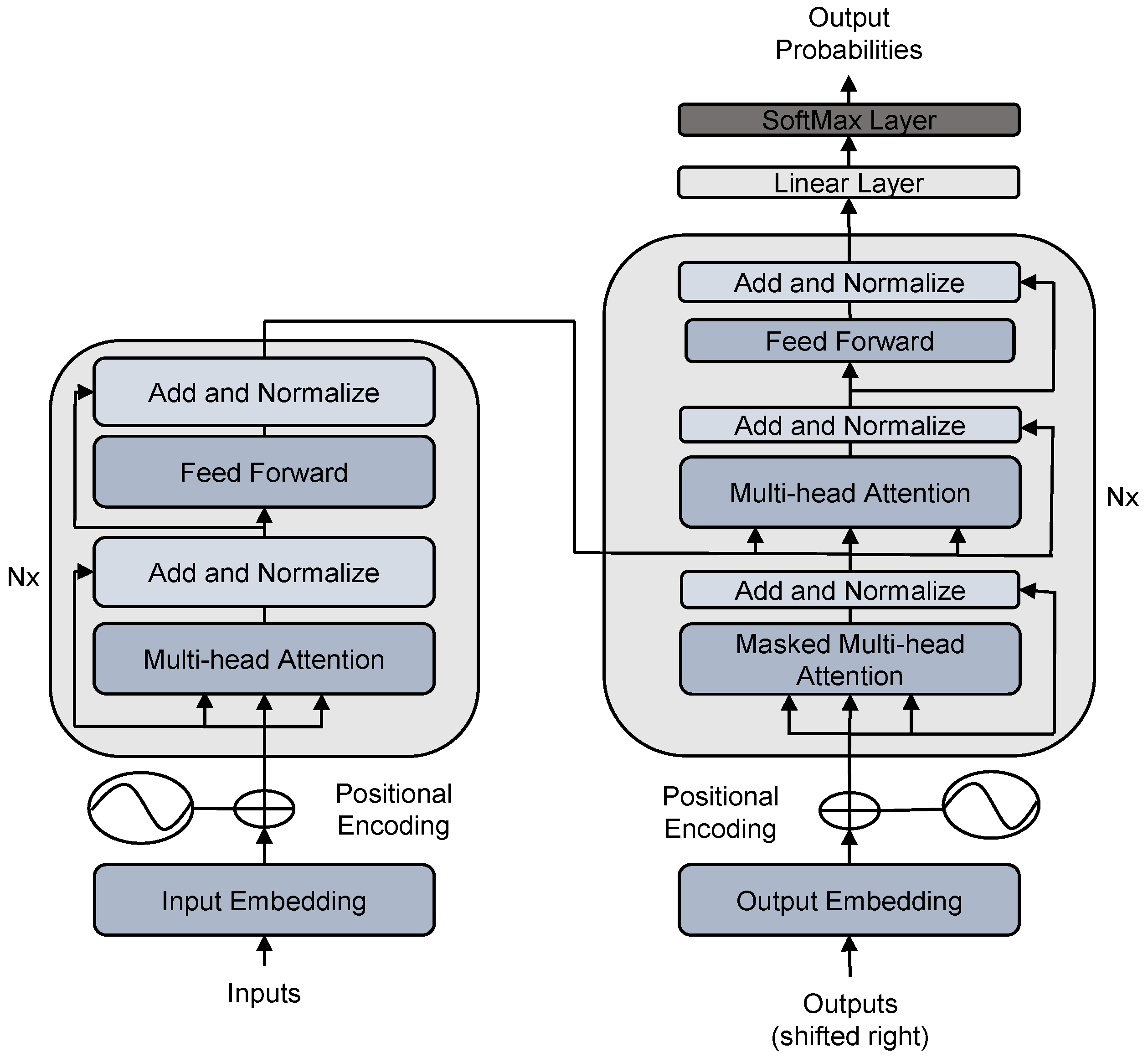
2.1. Types of Transformers
- -
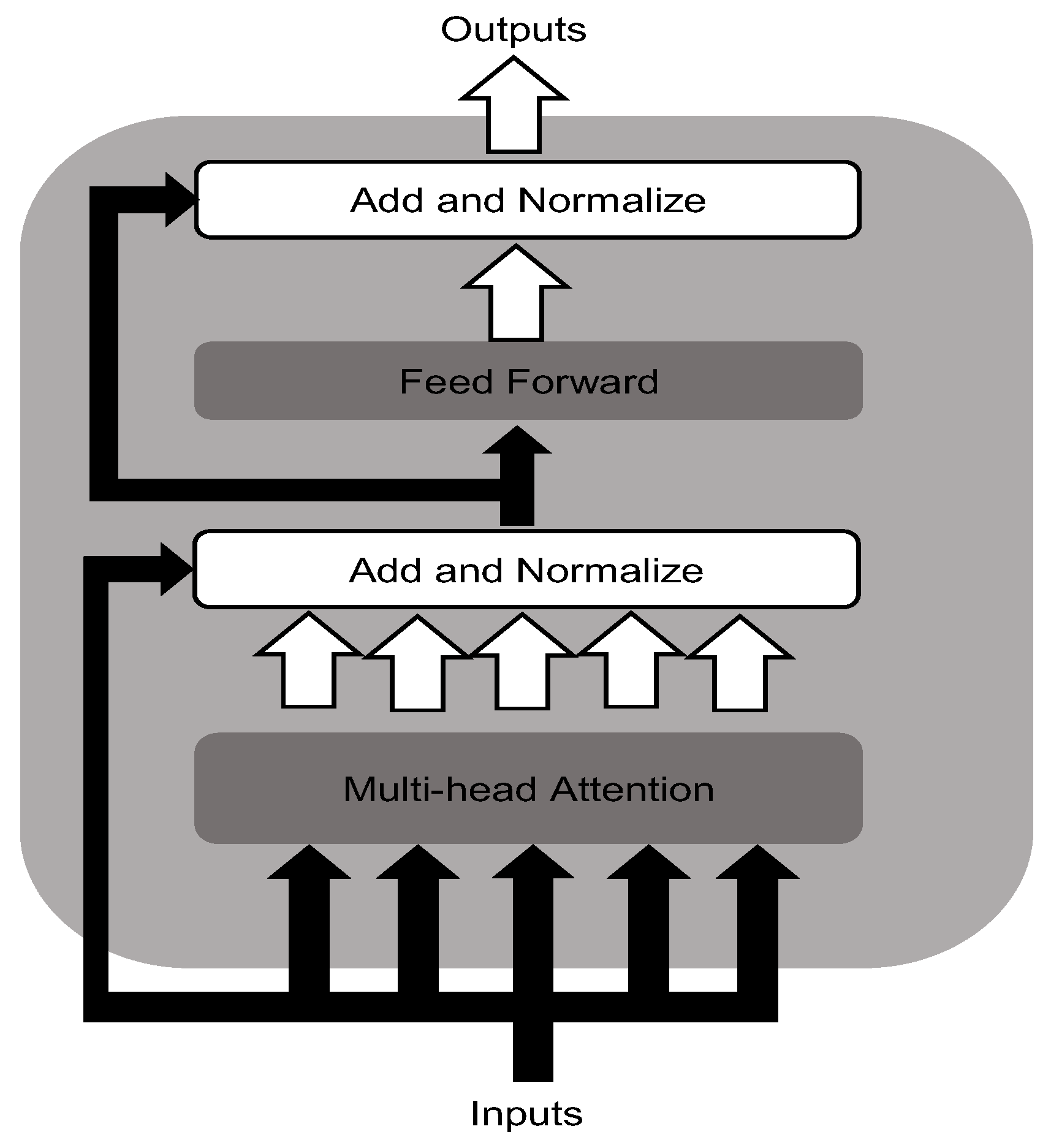
- Encoder-only: This model can convert an input sequence of text into a numerical representation suitable for tasks such as text classification or named entity recognition. The representation calculated for a given token in this architecture depends on bidirectional attention, meaning it relies on both the left and right context of the token.
- -
- Decoder-only: This type of model is capable of automatically completing a sequence by iteratively predicting the most probable next word. In this case, the model relies on causal or autoregressive attention, meaning that the representation calculated for a token in this architecture depends solely on the left context.
- -
- Encoder–decoder: these are used to model complex mappings from one sequence of text to another, making them suitable for tasks such as machine translation and summarization.
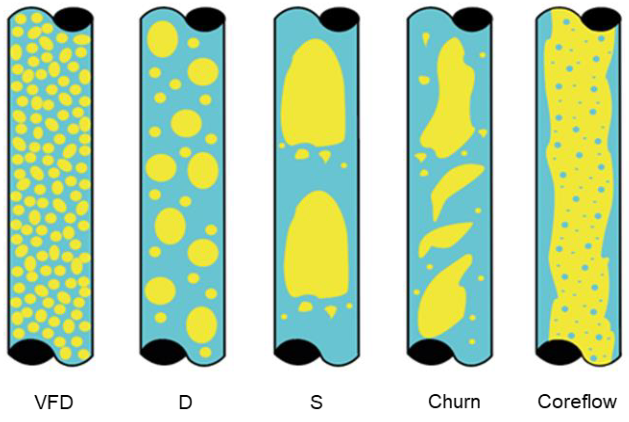
2.2. Data Structure
2.3. Transformer Neural Network Model
3. Results
4. Conclusions
Author Contributions
Funding
Data Availability Statement
Conflicts of Interest
References
- Rosa, E.S. Escoamento Multifásico Isotérmico: Modelos de Multifluidos e de Mistura; Bookman: Porto Alegre, Brasil, 2012; ISBN 9788540700703. [Google Scholar]
- Hernández-Cely, M.M.; Ruiz-Díaz, C. Estudio de los fluidos aceite-agua a través del sensor basado en la permitividad eléctrica del patrón de fluido. Rev. UIS Ing. 2020, 19, 177–186. [Google Scholar] [CrossRef]
- Santos, D.S.; Faia, P.M.; Garcia, F.A.P.; Rasteiro, M.G. Oil/water stratified flow in a horizontal pipe: Simulated and experimental studies using EIT. J. Pet. Sci. Eng. 2019, 174, 1179–1193. [Google Scholar] [CrossRef]
- Liu, H.; Duan, J.; Li, J.; Gu, K.; Lin, K.; Wang, J.; Yan, H.; Guan, L.; Li, C. Numerical quasi-three dimensional modeling of stratified oil-water flow in horizontal circular pipe. Ocean Eng. 2022, 251, 111172. [Google Scholar] [CrossRef]
- Obaseki, M.; Elijah, P.T.; Alfred, P.B. Development of model to eliminate sand trapping in horizontal fluid pipelines. J. King Saud Univ.-Eng. Sci. 2022, 34, 425–434. [Google Scholar] [CrossRef]
- Gomez, C.; Ruiz, D.; Cely, M. Specialist system in flow pattern identification using artificial neural Networks. J. Appl. Eng. Sci. 2023, 21, 285–299. [Google Scholar] [CrossRef]
- Bazon, P.B.; Castro-Bolivar, J.E.; Ruiz-Diaz, C.M.; Hernández-Cely, M.M.; Rodriguez, O.M.H. Hybrid machine learning model applied to phase inversion prediction in liquid-liquid pipe flow. Multiph. Sci. Technol. 2023, 35, 35–53. [Google Scholar] [CrossRef]
- de Almeida Coelho, N.M.; Taqueda, M.E.S.; Souza, N.M.O.; de Paiva, J.L.; Santos, A.R.; Lia, L.R.B.; de Moraes, M.S.; de Moraes Júnior, D. Energy savings on heavy oil transportation through core annular flow pattern: An experimental approach. Int. J. Multiph. Flow 2020, 122, 103127. [Google Scholar] [CrossRef]
- Sánchez, E.; Romero, C.; Zeppieri, S.; González-Mendizabal, D. Estudio experimental sobre patrones de flujo líquido-líquido en tuberias verticales. In Proceedings of the 8° Congreso Iberoamericano de Ingeniería Mecánica; Universidad Pontificia del Peru: Cusco, Mexico, 2007. [Google Scholar]
- Ruiz-Díaz, C.; Hernández-Cely, M.M.; González-Estrada, O.A. Modelo predictivo para el cálculo de la fracción volumétrica de un flujo bifásico agua- aceite en la horizontal utilizando una red neuronal artificial. Rev. UIS Ing. 2022, 21, 155–164. [Google Scholar] [CrossRef]
- Sanguino, V. Modelamiento en CFD de Flujo Bifásico (Aceite-Agua) en una Tubería Vertical. Bachelor’s Thesis, Universidad de los Andes, Bogotá, Colombia, 2014. [Google Scholar]
- Vasheghani Farahani, M.; Jahanpeyma, Y.; Taghikhani, V. Dynamic Modeling and Numerical Simulation of Gas Lift Performance in Deviated Oil Well Using the Two-Fluid Model. In Proceedings of the 80th EAGE Conference and Exhibition 2018, Copenhagen, Denmark, 11–14 June 2018; European Association of Geoscientists & Engineers: Utrecht, The Netherlands, 2018. [Google Scholar] [CrossRef]
- Hassanpouryouzband, A.; Yang, J.; Tohidi, B.; Chuvilin, E.; Istomin, V.; Bukhanov, B. Geological CO2 Capture and Storage with Flue Gas Hydrate Formation in Frozen and Unfrozen Sediments: Method Development, Real Time-Scale Kinetic Characteristics, Efficiency, and Clathrate Structural Transition. ACS Sustain. Chem. Eng. 2019, 7, 5338–5345. [Google Scholar] [CrossRef]
- Hassanpouryouzband, A.; Joonaki, E.; Taghikhani, V.; Bozorgmehry Boozarjomehry, R.; Chapoy, A.; Tohidi, B. New Two-Dimensional Particle-Scale Model To Simulate Asphaltene Deposition in Wellbores and Pipelines. Energy Fuels 2018, 32, 2661–2672. [Google Scholar] [CrossRef]
- Norouzi, S.; Nazari, M.; VasheghaniFarahani, M. A Novel Hybrid Particle Swarm Optimization-Simulated Annealing Approach for CO2-Oil Minimum Miscibility Pressure (MMP) Prediction. In Proceedings of the 81st EAGE Conference and Exhibition 2019, London, UK, 3–6 June 2019; European Association of Geoscientists & Engineers: Utrecht, The Netherlands, 2019; pp. 1–5. [Google Scholar] [CrossRef]
- Sossa, J. El papel de la inteligencia artificial en la Industria 4.0. In Inteligencia Artificial y Datos Masivos en Archivos Digitales Sonoros y Audiovisuales; Rodríguez Reséndiz, P.O., Ed.; Univ. Nacional Autónoma de México: Mexico City, Mexico, 2020. [Google Scholar]
- Valle Tamayo, G.A.; Romero Consuegra, F.; Cabarcas Simancas, M.E. Predicción de flujo multifásico en sistemas de recolección de crudo: Descripción de requerimientos. Rev. Fuentes Reventón Energético 2017, 15, 87–99. [Google Scholar] [CrossRef]
- Ruiz-Diaz, C.M.; Hernández-Cely, M.M.; González-Estrada, O.A. A Predictive Model for the Identification of the Volume Fraction in Two-Phase Flow. Cienc. Desarro. 2021, 12, 49–55. [Google Scholar]
- Jahanandish, I.; Salimifard, B.; Jalalifar, H. Predicting bottomhole pressure in vertical multiphase flowing wells using artificial neural networks. J. Pet. Sci. Eng. 2011, 75, 336–342. [Google Scholar] [CrossRef]
- Semeraro, F.; Griffiths, A.; Cangelosi, A. Human–robot collaboration and machine learning: A systematic review of recent research. Robot. Comput. Integr. Manuf. 2022, 79, 102432. [Google Scholar] [CrossRef]
- Vaswani, A.; Shazeer, N.; Parmar, N.; Uszkoreit, J.; Jones, L.; Gomez, A.N.; Kaiser, L.; Polosukhin, I. Attention is All you Need. In Proceedings of the Advances in Neural Information Processing Systems 30: Annual Conference on Neural Information Processing Systems 2017, Long Beach, CA, USA, 4–9 December 2017; Guyon, I., von Luxburg, U., Bengio, S., Wallach, H.M., Fergus, R., Vishwanathan, S.V.N., Garnett, R., Eds.; Curran Associates, Inc.: Red Hook, NY, USA, 2017; pp. 5998–6008. [Google Scholar]
- Lakew, S.M.; Cettolo, M.; Federico, M. A comparison of transformer and recurrent neural networks on multilingual neural machine translation. In Proceedings of the COLING 2018—27th International Conference on Computational Linguistics, Santa Fe, NM, USA, 20–26 August 2018; pp. 641–652. [Google Scholar]
- Brown, T.B.; Mann, B.; Ryder, N.; Subbiah, M.; Kaplan, J.; Dhariwal, P.; Neelakantan, A.; Shyam, P.; Sastry, G.; Askell, A.; et al. Language models are few-shot learners. Adv. Neural Inf. Process. Syst. 2020, 2020, 1154–1156. [Google Scholar]
- Safi Samghabadi, N.; Patwa, P.; Pykl, S.; Mukherjee, P.; Das, A.; Solorio, T. Aggression and Misogyny Detection using BERT: A Multi-Task Approach. In Proceedings of the Second Workshop on Trolling, Aggression and Cyberbullying; European Language Resources Association (ELRA): Marseille, France, 2020; pp. 126–131. [Google Scholar]
- Meng, L.; Li, H.; Chen, B.-C.; Lan, S.; Wu, Z.; Jiang, Y.-G.; Lim, S.-N. AdaViT: Adaptive Vision Transformers for Efficient Image Recognition. In Proceedings of the IEEE/CVF Conference on Computer Vision and Pattern Recognition (CVPR), Nashville, TN, USA, 20–25 June 2021; pp. 12309–12318. [Google Scholar]
- Le, N.Q.K.; Ho, Q.T. Deep transformers and convolutional neural network in identifying DNA N6-methyladenine sites in cross-species genomes. Methods 2022, 204, 199–206. [Google Scholar] [CrossRef] [PubMed]
- Sharma, A.; Jain, P.; Mahgoub, A.; Zhou, Z.; Mahadik, K.; Chaterji, S. Lerna: Transformer architectures for configuring error correction tools for short- and long-read genome sequencing. BMC Bioinform. 2022, 23, 25. [Google Scholar] [CrossRef]
- Behjati, A.; Zare-Mirakabad, F.; Arab, S.S.; Nowzari-Dalini, A. Protein sequence profile prediction using ProtAlbert transformer. Comput. Biol. Chem. 2022, 99, 107717. [Google Scholar] [CrossRef]
- Qu, K.; Si, G.; Shan, Z.; Kong, X.G.; Yang, X. Short-term forecasting for multiple wind farms based on transformer model. Energy Rep. 2022, 8, 483–490. [Google Scholar] [CrossRef]
- Wang, L.; He, Y.; Li, L.; Liu, X.; Zhao, Y. A novel approach to ultra-short-term multi-step wind power predictions based on encoder–decoder architecture in natural language processing. J. Clean. Prod. 2022, 354, 131723. [Google Scholar] [CrossRef]
- Gomaa, I.; Gowida, A.; Elkatatny, S.; Abdulraheem, A. The prediction of wellhead pressure for multiphase flow of vertical wells using artificial neural networks. J. Geosci. 2021, 14, 1–10. [Google Scholar] [CrossRef]
- Tunstall, L.; Von Werra, L.; Wolf, T. Natural Language Processing with Transformers: Building Language Applications with Hugging Face; O’Reilly: Sebastopol, CA, USA, 2022; ISBN 978-1-098-10324-8. [Google Scholar]
- Bannwart, A.C.; Rodriguez, O.M.H.; de Carvalho, C.H.M.; Wang, I.S.; Vara, R.M.O. Flow Patterns in Heavy Crude Oil-Water Flow. J. Energy Resour. Technol. 2004, 126, 184–189. [Google Scholar] [CrossRef]
- Abduvayt, P.; Manabe, R.; Watanabe, T.; Arihara, N. Analisis of Oil-Water Flow Tests in Horizontal, Hilly-Terrain, and Vertical Pipes. In Proceedings of the SPE Annual Technical Conference and Exhibition; Society of Petroleum Engineers: London, UK, 2004; pp. 1335–1347. [Google Scholar] [CrossRef]
- Du, M.; Jin, N.-D.; Gao, Z.-K.; Wang, Z.-Y.; Zhai, L.-S. Flow pattern and water holdup measurements of vertical upward oil–water two-phase flow in small diameter pipes. Int. J. Multiph. Flow 2012, 41, 91–105. [Google Scholar] [CrossRef]
- Flores, J.; Chen, X.; Brill, J. Characterization of Oil-Water Flow Patterns in Vertical and Deviated Wells. In Proceedings of the SPE Annual Technical Conference and Exhibition; Society of Petroleum Engineers: London, UK, 1997; Volume 1, pp. 55–64. [Google Scholar] [CrossRef]
- Ganat, T.; Ridha, S.; Hairir, M.; Arisa, J.; Gholami, R. Experimental investigation of high-viscosity oil–water flow in vertical pipes: Flow patterns and pressure gradient. J. Pet. Explor. Prod. Technol. 2019, 9, 2911–2918. [Google Scholar] [CrossRef]
- Govier, G.W.; Sullivan, G.A.; Wood, R.K. The upward vertical flow of oil-water mixtures. Can. J. Chem. Eng. 1961, 39, 67–75. [Google Scholar] [CrossRef]
- Han, Y.F.; Jin, N.D.; Zhai, L.S.; Zhang, H.X.; Ren, Y.Y. Flow pattern and holdup phenomena of low velocity oil-water flows in a vertical upward small diameter pipe. J. Pet. Sci. Eng. 2017, 159, 387–408. [Google Scholar] [CrossRef]
- Hasan, A.R.; Kabir, C.S. A New Model for Two-Phase Oil/Water Flow: Production Log Interpretation nd Tubular Calculations. SPE Prod. Eng. 1990, 5, 193–199. [Google Scholar] [CrossRef]
- Hasan, A.R.; Kabir, C.S. A simplified model for oil/water flow in vertical and deviated wellbores. SPE Prod. Facil. 1999, 14, 56–62. [Google Scholar] [CrossRef]
- Jana, A.K.; Das, G.; Das, P.K. Flow regime identification of two-phase liquid–liquid upflow through vertical pipe. Chem. Eng. Sci. 2006, 61, 1500–1515. [Google Scholar] [CrossRef]
- Jana, A.K.; Ghoshal, P.; Das, G.; Das, P.K. An Analysis of Pressure Drop and Holdup for Liquid-Liquid Upflow through Vertical Pipes. Chem. Eng. Technol. 2007, 30, 920–925. [Google Scholar] [CrossRef]
- Guo, J.; Yang, Y.; Zhang, S.; Zhang, D.; Cao, C.; Ren, B.; Liu, L.; Xing, Y.; Xiong, R. Heavy oil-water flow patterns in a small diameter vertical pipe under high temperature/pressure conditions. J. Pet. Sci. Eng. 2018, 171, 1350–1365. [Google Scholar] [CrossRef]
- Mazza, R.A.; Suguimoto, F.K. Experimental investigations of kerosene-water two-phase flow in vertical pipe. J. Pet. Sci. Eng. 2020, 184, 106580. [Google Scholar] [CrossRef]
- Mydlarz-Gabryk, K.; Pietrzak, M.; Troniewski, L. Study on oil–water two-phase upflow in vertical pipes. J. Pet. Sci. Eng. 2014, 117, 28–36. [Google Scholar] [CrossRef]
- Rodriguez, O.M.H.; Bannwart, A.C. Experimental study on interfacial waves in vertical core flow. J. Pet. Sci. Eng. 2006, 54, 140–148. [Google Scholar] [CrossRef]
- Xu, J.; Li, D.; Guo, J.; Wu, Y. Investigations of phase inversion and frictional pressure gradients in upward and downward oil–water flow in vertical pipes. Int. J. Multiph. Flow 2010, 36, 930–939. [Google Scholar] [CrossRef]
- Yang, Y.; Guo, J.; Ren, B.; Zhang, S.; Xiong, R.; Zhang, D.; Cao, C.; Liao, Z.; Zhang, S.; Fu, S. Oil-Water flow patterns, holdups and frictional pressure gradients in a vertical pipe under high temperature/pressure conditions. Exp. Therm. Fluid Sci. 2019, 100, 271–291. [Google Scholar] [CrossRef]
- Zhao, D.; Guo, L.; Hu, X.; Zhang, X.; Wang, X. Experimental study on local characteristics of oil-water dispersed flow in a vertical pipe. Int. J. Multiph. Flow 2006, 32, 1254–1268. [Google Scholar] [CrossRef]


| Reference | D [m] | [Pa·s] | Number of Flow Patterns | Data | |
|---|---|---|---|---|---|
| [33] | 0.0284 | 0.488 | 925 | 3 | 392 |
| [34] | 0.1064 | 0.00188 | 800 | 6 | 49 |
| [35] | 0.02 | 0.011 | 856 | 3 | 101 |
| [36] | 0.05 | 0.02 | 850 | 5 | 126 |
| [37] | 0.04 | 0.035 | 860 | 4 | 92 |
| [38] | 0.0263 | 0.0201 | 851 | 2 | 15 |
| [39] | 0.02 | 0.125 | 801 | 4 | 175 |
| [40] | 0.127 | 0.001 | 801 | 2 | 9 |
| [41] | 0.027 | 0.02 | 801 | 4 | 109 |
| [42] | 0.0254 | 0.001 | 792 | 4 | 55 |
| [43] | 0.0254 | 0.001 | 792 | 5 | 32 |
| [44] | 0.01 | 0.287 | 1823 | 3 | 1421 |
| [45] | 0.026 | 0.0011 | 793 | 5 | 90 |
| [46] | 0.03 | 0.03 | 856 | 4 | 252 |
| [47] | 0.0284 | 0.5 | 930 | 1 | 92 |
| [48] | 0.03 | 0.044 | 860 | 4 | 98 |
| [49] | 0.02 | 0.09732 | 857 | 7 | 1699 |
| [50] | 0.04 | 0.0041 | 824 | 1 | 57 |
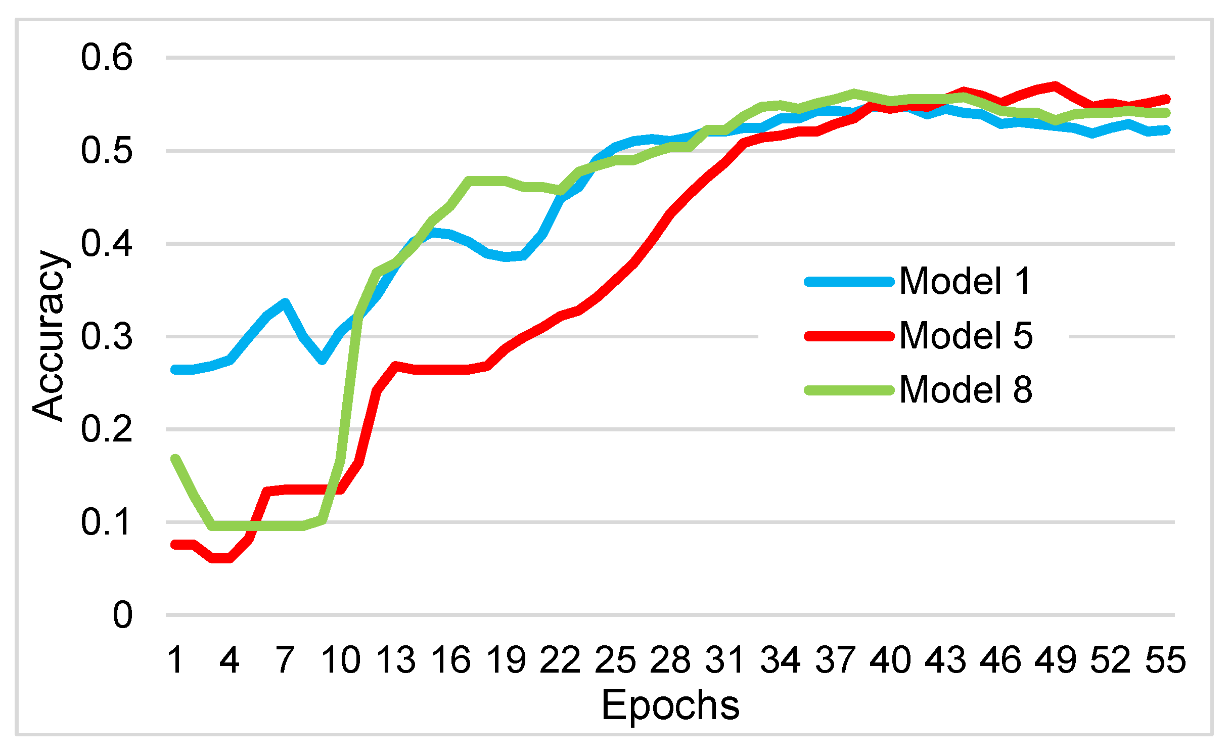
| Parameters | Model 1 | Model 2 | Model 3 | Model 4 | Model 5 | Model 6 | Model 7 | Model 8 |
|---|---|---|---|---|---|---|---|---|
| Activation function | sigmoid | ReLU | sigmoid | ReLU | sigmoid | Tanh | Gelu | ReLU |
| N° attention heads | 2 | 4 | 4 | 4 | 1 | 2 | 2 | 2 |
| Dropout | 0.3 | 0.5 | 0.5 | 0.1 | 0.1 | 0.3 | 0.3 | 0.1 |
| Learning rate | 0.001 | 0.001 | 0.001 | 0.0005 | 0.001 | 0.001 | 0.001 | 0.001 |
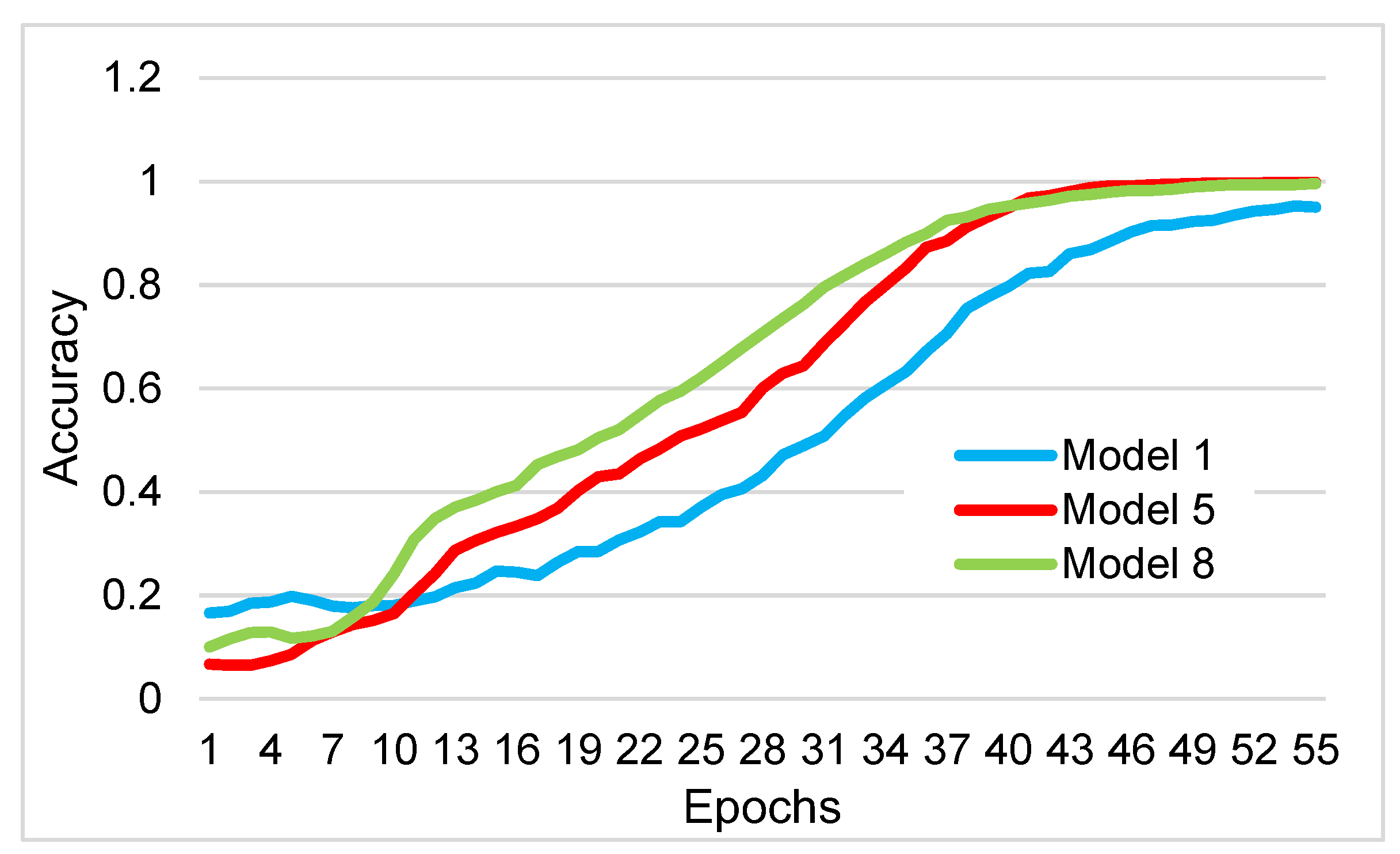
| Training accuracy (%) | 99.92 | 99.54 | 99.49 | 99.38 | 99.97 | 99.61 | 99.72 | 99.97 |
| Test accuracy (%) | 52.25 | 51.23 | 51.43 | 51.64 | 55.53 | 52.87 | 49.80 | 54.10 |
| Validation accuracy (%) | 51.04 | 48.98 | 49.18 | 52.87 | 52.25 | 50.00 | 48.98 | 53.07 |
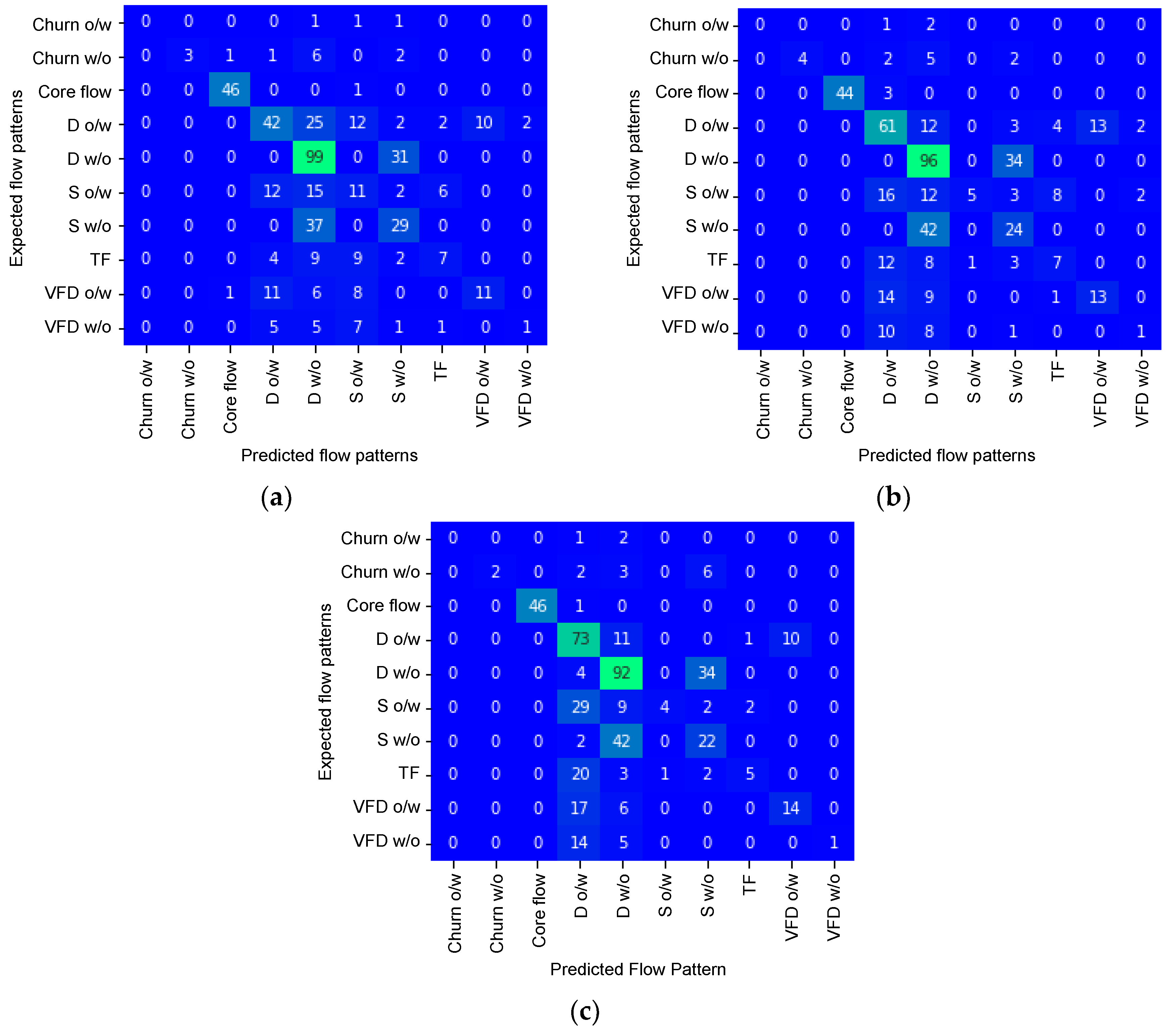
| Model 1 | Model 5 | Model 8 | ||||
|---|---|---|---|---|---|---|
| Precision [%] | Accuracy [%] | Precision [%] | Accuracy [%] | Precision [%] | Accuracy [%] | |
| Churn o/w | 0.00 | 98.81 | 0.00 | 98.84 | 0.00 | 98.85 |
| Churn w/o | 100.00 | 96.14 | 100.00 | 96.59 | 100.00 | 95.93 |
| Core flow | 95.83 | 98.81 | 100.00 | 98.84 | 100.00 | 99.62 |
| D o/w | 56.00 | 74.33 | 51.26 | 73.49 | 44.79 | 70.00 |
| D w/o | 48.77 | 64.84 | 49.48 | 65.89 | 53.18 | 68.52 |
| S o/w | 22.45 | 77.33 | 83.33 | 85.86 | 80.00 | 85.76 |
| S w/o | 41.43 | 76.15 | 34.29 | 74.34 | 33.33 | 74.64 |
| TF | 43.75 | 88.30 | 35.00 | 87.33 | 62.50 | 89.93 |
| VFD o/w | 52.38 | 87.37 | 50.00 | 87.33 | 58.33 | 88.70 |
| VFD w/o | 33.33 | 92.25 | 20.00 | 91.76 | 100.00 | 93.17 |
| Average | 49.39 | 85.43 | 52.34 | 86.03 | 63.21 | 86.51 |
Disclaimer/Publisher’s Note: The statements, opinions and data contained in all publications are solely those of the individual author(s) and contributor(s) and not of MDPI and/or the editor(s). MDPI and/or the editor(s) disclaim responsibility for any injury to people or property resulting from any ideas, methods, instructions or products referred to in the content. |
© 2024 by the authors. Licensee MDPI, Basel, Switzerland. This article is an open access article distributed under the terms and conditions of the Creative Commons Attribution (CC BY) license (https://creativecommons.org/licenses/by/4.0/).
Share and Cite
Ruiz-Díaz, C.M.; Perilla-Plata, E.E.; González-Estrada, O.A. Two-Phase Flow Pattern Identification in Vertical Pipes Using Transformer Neural Networks. Inventions 2024, 9, 15. https://doi.org/10.3390/inventions9010015
Ruiz-Díaz CM, Perilla-Plata EE, González-Estrada OA. Two-Phase Flow Pattern Identification in Vertical Pipes Using Transformer Neural Networks. Inventions. 2024; 9(1):15. https://doi.org/10.3390/inventions9010015
Chicago/Turabian StyleRuiz-Díaz, Carlos Mauricio, Erwing Eduardo Perilla-Plata, and Octavio Andrés González-Estrada. 2024. "Two-Phase Flow Pattern Identification in Vertical Pipes Using Transformer Neural Networks" Inventions 9, no. 1: 15. https://doi.org/10.3390/inventions9010015
APA StyleRuiz-Díaz, C. M., Perilla-Plata, E. E., & González-Estrada, O. A. (2024). Two-Phase Flow Pattern Identification in Vertical Pipes Using Transformer Neural Networks. Inventions, 9(1), 15. https://doi.org/10.3390/inventions9010015