Abstract
Predictions are presented of mean values of statistical variables of large-scale turbulent flow of the widely used basic k- model, and of a new model, which is based on general statistical descriptions of turbulence. The predictions are verified against published results of direct numerical simulations (DNSs) of Navier–Stokes equations. The verification concerns turbulent channel flow at shear Reynolds numbers of 950, 2000, and . The basic k- model is largely based on empirical formulations accompanied by calibration constants. This contrasts with the new model, where descriptions of leading statistical quantities are based on the general principles of statistical turbulence at a large Reynolds number and stochastic theory. Predicted values of major output variables such as turbulent viscosity, diffusivity of passive admixture, temperature, and fluid velocities compare well with DNS for the new model. Significant differences are seen for the basic k- model.
1. Introduction
The description of turbulence has been an issue right from the beginning. A solid starting point for analysis is the Navier–Stokes equations, which describe the flow. These can be time-averaged, resulting in equations for mean values of velocity, pressure, and temperature. The problem arises with the average values of the products of fluctuating quantities within the non-linear convection terms in the equations. They describe the effect of fluctuations on mean flow quantities. The proposed representations of average nonlinear convective fluctuations are of a hypothetical nature, drawing analogies with molecular chaos. Boussinesq [1] was the first to follow this line of thinking by introducing the gradient hypothesis: the averaged nonlinear fluxes are proportional to the derivative of the mean flow quantity, preceded by a constant termed the turbulent viscosity or turbulent diffusion coefficient. Several versions and extensions based on the same idea have since been put forward by the pioneers of turbulence theory: Taylor [2], Prandtl [3], and von Karman [4], among others. They also form the basis of many of today’s computer models used in engineering and environmental analyses; for example, see the books of Hanjalic and Launder [5] and Bernard and Wallace [6].
An offspring of the aforementioned concept is the basic k- model, which is widely used in engineering and environmental analyses [5,6]. This model describes the average value of momentum fluxes through the gradient of the mean velocity. Fluctuations are isotropic and the coefficient proceeding the gradient equals , where k is the mean kinetic energy of fluctuations, is the mean energy dissipation rate, and is a calibration constant. The model is completed by equations for k and . The gradient hypothesis is also applied to several other flux terms in equations with different values of calibration constants.
The problems with gradient-based models include their hypothetical origin and lack of uniqueness. Starting from a sketchy analogy with laminar diffusion, almost limitless forms of gradient representations and proceeding functional dependencies can be devised. A new development that surpasses these limitations is the statistical description of anisotropic inhomogeneous turbulence; see Brouwers [7,8,9]. Turbulence at a high Reynolds number is featured by unstable eddies of whirling irregular fluid velocities whose behaviors are governed by the domination of the inertial forces in the momentum balance; see Monin and Yaglom, Vol. II, Ch.8 [10]. The eddies start at sizes of the configuration and then break down to smaller ones until the point where viscous forces come into play at sizes of a few millimeters. Here, Kolmogorov’s theory of small viscous scales comes into play [10]. Building on this framework of high Reynolds turbulence and using the methods of the stochastic theory of Van Kampen [11] and Stratonovich [12], explicit statistical descriptions of governing variables are obtained. They are the leading terms of asymptotic expansions based on the small value of the inverse of the universal Lagrangian Kolmogorov constant. The results represent unique descriptions of turbulent flow statistics, subject to deviations due to truncated higher-order terms.
The results of direct numerical simulation (DNS) of the Navier–Stokes equations offer an opportunity for testing the outcomes of turbulence models. With the evolution of modern computing power, it has become possible to generate a wealth of accurate data on turbulent flow at high Reynolds numbers. The recent DNS data of the turbulent channel flow of Hoyas et al. [13,14] and Kuerten et al. [15] are particularly noteworthy. Fluctuating channel velocities are strongly anisotropic and averages of flow quantities vary strongly with distance from the wall. Inhomogeneity and anisotropy are characteristics of turbulence, in practice. The DNS data provide a meaningful test case for models. In this paper, a detailed comparison is presented of the DNS data, along with predictions of the basic k- model and the new model based on general statistical descriptions, referred to as the fundamental model.
2. The Basic - Model and the New Fundamental Model
The turbulent flow of an incompressible or nearly incompressible fluid, e.g., a liquid or gas flowing at speeds where the square of the Mach number is minimal, is considered. The density is assumed to be constant. Turbulent fluctuations measured at a fixed point in space are treated as a statistical process that is stationary or almost stationary in time compared to the time of velocity fluctuations. Statistical averages follow from time-averaging over sufficiently long time intervals. The time-averaged representation of the Navier–Stokes equations is given by the following:
- Conservation of mass:
- Conservation of momentum:
- Conservation of energy:
2.1. Turbulent Diffusion in the Basic k- Model
The appearance of turbulent fluxes—in the convection terms of the averaged conservation equations—results in an unclosed set of equations for mean flow variables. It is known as the closure problem. To resolve this issue, a diffusion hypothesis has been introduced in the basic k- model. In this hypothesis, turbulent fluxes are treated as isotropic and are described by [5,6].
where is a scalar that represents diffusivity or turbulent viscosity, which is defined by the following:
where k is the average kinetic energy of fluctuations, , and denotes the average energy dissipation rate, with being kinematic viscosity; in (4) and (5) is a calibration constant whose value is usually taken as [5,6]. In Equation (5), correction factors are sometimes added to the diffusion constant, i.e., a turbulent Prandtl number and a turbulent Schmidt number for temperature and admixture, respectively. But these numbers are generally close to unity and are omitted here.
2.2. Turbulent Diffusion in the Fundamental Model
The derivation of the fundamental model starts from a Langevin equation for fluid particle velocity [8,9,10]. In this equation, the limiting form of Kolmogorov’s theory of small scales is implemented, i.e., where the characteristic times for velocity fluctuations are much larger than the times of viscous scales. This is the case when the Reynolds number is large; see Kolmogorov [16]. One further step involves an expansion, in terms of the inverse of the Kolmogorov constant . Matching predictions with measurements and DNS data reveal values of at around 6–7; in the present analysis, a value of 7 is adopted. Furthermore, the area where the Lagrangian description applies can be reduced to a point in the Eulerian flow description in the limit of small . In this way, Lagrangian-based descriptions are connected to Eulerian ones. The following descriptions for the flux terms are obtained [8,9]
where the fundamentally based diffusion tensor, , is described by the following:
and
is covariance or Reynolds stress. Relations (8)–(10) are part of the description, which holds in the entire flow configuration (except the thin viscous layers at walls) once they are coupled to conservation Equations (1)–(3). In this way, the turbulent flux change at each point, x, as described by (7) and (8), is connected to the kinetic energy and energy dissipation changes. Although the presence of in the expression for energy dissipation may suggest otherwise, is a characteristic of the main inviscid flow outside the boundary layers [10]. The magnitude of velocity gradients in turbulence is governed by the small viscous scales. It scales as and makes the magnitude of independent of . This independence is reflected in the equations for k and , presented in the next section.
The above expressions for the diffusion of the fundamental model reveal the dependency on mean gradients, which are of a more complex structure than those in the basic k- model. This reflects the anisotropy of the fluctuating velocity field and reveals a more complex dependency on flow statistics.
The application of the fundamentally based diffusion approximation to a scalar, as conducted in Equation (8), is only justified if the scalar is conservative [8,9]. The value of the conservative scalar is constant when following a fluid particle and fluctuates in value in a fixed coordinate system due to fluid particle fluctuations. This is the case for temperature in an incompressible fluid such as liquids. It is approximately correct if the fluid is almost incompressible, as is the case in gases flowing at speeds where the square of the Mach number is small. The scalar representation can also be applied to passive or almost passive admixtures in fluids, such as aerosols in air [7,8,9]. It leads to errors when applied to non-conservative scalars such as kinetic energy and pressure; see Section 5.
3. Equations for and
Incorporating the expressions for turbulent diffusion from the basic k- model and the fundamental model into the averaged conservation equations introduces two unknowns: the mean kinetic energy, k, and the mean energy dissipation rate, . Equations for k and can be obtained from the Navier–Stokes equations [8,9]. Our aim is to describe flow away from the thin, viscous layers near walls, which are only a few millimeters. In line with this approach, the contributions in the equations for k and from laminar viscosity will be disregarded (as was conducted in the conservation Equations (1)–(3)). To provide boundary conditions at the wall, the viscous layer is surpassed by applying the solutions of the log layer at : [5,6].
The equation for k reads as follows [5,6]:
where P is the mean production of turbulent fluctuations, defined by the following:
and where and are the fluctuating parts of kinetic energy and pressure, respectively, which are the kinetic energy and dissipation rates minus their time-averaged values. There are two turbulent flux terms in Equation (11), i.e., the third and fourth terms on the LHS of (11), which need to be modeled. In the basic k- model, both terms are lumped together [5,6] and are described by the following:
- Basic k-ϵ model
- Fundamental model
The theory underlying the fundamental model provides general expressions for turbulent scalar fluxes, which are free from calibration factors. However, these expressions are only valid for conservative scalars and lead to disagreement with DNS results when applied to turbulent fluxes of kinetic energy and pressure [8]. A fallback to empirical construction is needed. It reads as follows:
where it is noted that if k was a conserved scalar, its diffusion should be described by . Factor represents correction for non-conservative behavior and includes the relatively small contribution of pressure diffusion [8]. The above relations for the diffusion of kinetic energy and pressure will be compared and calibrated with the DNS results in Section 5.
The equation for , conventionally applied in CFD models, is largely an empirical construction [5,6]. Its basic form follows from the Navier–Stokes equations. It contains a number of terms that are governed by small viscous scales. These terms are generally replaced by expressions that meet the criteria of matching the results of decaying grid turbulence and the log layer of turbulent channel flow. The equation reads as follows:
- Basic k-ϵ model
- Fundamental model
4. Channel Flow
The objective is to compare the results of the basic k- model and the fundamental model with those of the DNS of the channel flow. The channel consists of parallel planes in between, where the mean velocity, , is unidirectional in the direction, , parallel to the planes. Its magnitude and the value of statistical averages related to velocity fluctuations only change in the direction, , normal to the planes. For channel flow, there is an exact solution for the mean pressure [9], which reads as follows:
where is shear velocity and is channel height. The shear velocity is determined by the pressure drop in direction at a given . There are theoretical and experimentally confirmed relations for the relationship determining . Another exact result for the channel flow is the description of the covariance, or .
which is valid outside the thin viscous layer at the wall, [9].
In the subsequent analysis of channel flow, we shall make use of dimensionless formulations: is made dimensionless by , and by , and by H, and P and by ; the subscript 2 of will be dropped. In this new notation, Equations (18) and (19) are as follows:
which is valid outside the thin viscous layer at the wall.
Furthermore, Equation (12) becomes
The above solutions follow from the averaged momentum equations adapted to the case of channel flow [9]. A complete specification of all variables follows from the expressions for turbulent fluxes and the equations for k and . In the case of channel flow, these reduce to the following:
- Basic k-ϵ model
- Fundamental model:
5. Testing the Diffusion Representations by DNS
In deriving equations for the mean values of flow quantities, the diffusion representation of mean fluxes has been used, i.e., the mean value of products of fluctuating quantities. Their correctness and accuracy will be assessed by comparing with the DNS results published for friction Reynolds numbers, of 950 [15], 2000 [13], and [14]. The comparison focuses on the flow in the main region—the region outside the thin boundary layer at the wall. In the main region, flow statistics are governed by unstable large eddies governed by inertia forces, while the effect of viscosity in this region is negligibly small. The presented basic k- as well as the fundamental model intend to describe these statistics. The boundary layer is governed by viscous forces and is situated in the region ; that is, and for and , respectively. The DNS results of the boundary layer near are omitted in this analysis.
5.1. Diffusion of Momentum
In the case of channel flow, turbulent momentum transport is apparent in the equation, as follows:
where is turbulent viscosity according to the DNS results, which is the value calculated from Equation (25) when substituting the values of and obtained from DNS data. The value according to the basic k- model is given by Equation (6) and the value according to the fundamental model is given by Equation (24g), where the RHSs of these equations are evaluated from the DNS data. The DNS data used are those of [14]. The three calculated turbulent viscosities are shown as functions of x in Figure 1. The ratios and versus x are shown in Figure 2. Disregarding the thin viscous layer at the wall, the fundamental model gives satisfactory agreement over the entire x range without the use of calibration factors. Deviations are less than from the DNS results. They can be ascribed to the truncation of higher-order terms in the expansions in powers of , which were used in the theory that led to the presented expressions [8,9]. The same conclusion was arrived at when using the DNS data of [9,13]. The basic k- model, on the other hand, disagrees quite a lot with DNS. The disagreement is the largest at small x values and gradually becomes smaller when approaching the central axis of the channel: . The dependency on x is apparently not well captured by representation (23d), in contrast with (24g), which shows satisfactory agreement over the entire range.
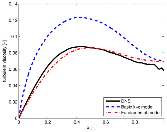
Figure 1.
Turbulent viscosities according to at , fundamental model , and the basic k- model versus the dimensionless distance from the wall, x. Results from DNS are represented by the solid line, results from the fundamental model are represented by a dash–dot line, and results from the basic k- model are represented by the dashed line.
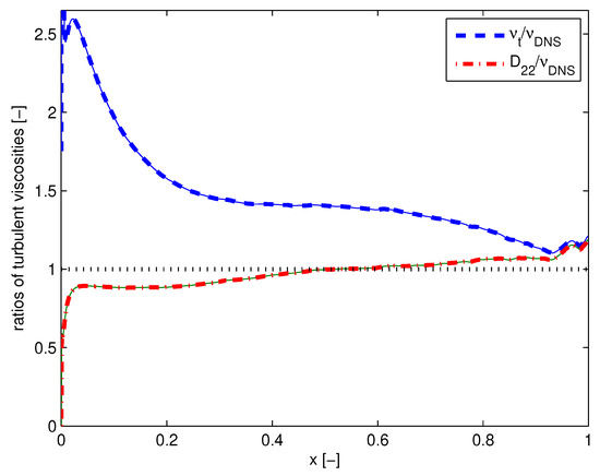
Figure 2.
Ratio of turbulent viscosity of the fundamental model to that of DNS at (lower line) and the ratio of turbulent viscosity of the basic k- model to that of DNS at (upper line) versus the dimensionless distance from the wall, x.
5.2. Diffusion of Temperature
Temperature is considered a conservative quantity in incompressible flow at high Reynolds numbers, where heat conductivity through molecular vibration is negligibly small outside thin layers at the walls. From the theory underlying the fundamental model, it follows that the thermal diffusion constant equals : cf. Equation (8). In the case of channel flow, it becomes and becomes equal to that of turbulent viscosity: cf. Equations (24d) and (24e). This result is confirmed by the Lagrangian-based DNS of channel flow at [15], where the thermal diffusion coefficient, according to DNS, is compared to that of the fundamentally based model, . The agreement closely resembles that shown in Figure 1 and Figure 2, c.q., and . Deviations of the predictions of the basic k- model are likely as equally large as those shown in Figure 1 and Figure 2.
5.3. Diffusion of Kinetic Energy and Pressure
In the basic k- model, fluxes of kinetic energy and pressure are lumped together, as shown in Equation (13). For channel flow, these terms become the following:
From Equation (14), we have the following for the fundamental model:
The description is used in the numerical solution of the equation for k in Section 6.
In Figure 3, we show the sum of both fluxes versus x, when the RHSs of (26) and (27) are evaluated by the DNS data. Values for the calibration constants and of 1 and were taken. Also, the value of the sums is obtained by the direct calculation of their values using the DNS of . The empirical construction of Equation (27), based on the fundamental model, offers surprisingly good agreement. The agreement extends over the entire x range and is obtained with the calibration constant, .
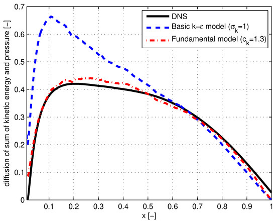
Figure 3.
Sum of turbulent fluxes of kinetic energy and pressure versus the dimensionless distance from the wall, x. The solid line is the sum according to DNS at , the dash–dot line is the empirical construction using the fundamental model, and the dashed line is the empirical construction of the basic k- model.
5.4. Diffusion of Energy Dissipation
DNS data do not provide information on the average values of products of velocity fluctuations and dissipation fluctuations. Direct verification of the diffusion representation is, thus, not possible. Further, the differential equation for mean energy dissipation in both models is largely an empirical construction. What remains possible is to verify the values of quantities derived from the solutions of the coupled differential equations for mean kinetic energy and mean energy dissipation rate against DNS data. This is the subject of the next section.
6. Solutions of and Compared with DNS
In the previous section, predictions of individual components of the models were verified by DNS. Further testing is executed by comparing numerically obtained solutions of the model equations as a whole with DNS.
6.1. Equations and Boundary Conditions
Model equations are given by coupled differential equations for mean kinetic energy and mean energy dissipation. For mean energy dissipation, the variable G is introduced, which is defined by the following:
Near the wall, outside the viscous layer, solutions should comply with the solutions of the log layer. Inertial subrange asymptotics [18] reveal that production, P, and dissipation, , are equal in this region: . Furthermore, , so that . DNS results show values of G in the log layer, which are between and 1 [13,14]. In the present analysis, the theoretical value of 1 is taken. Making use of relations (21), (23b), (23d), and (28), differential Equations (23e) and (23f) can be transformed into the following coupled equations for k and G, which are appropriate for the basic k- model.
- Basic k-ϵ model equations:
The equations appropriate for the fundamental model follow from (24h) and (24i) upon using (28), (21), (24a)–(24g).
- Fundamental model equations:
The value of follows from Equation (35) by letting x approach . It yields the following relation:
which is analogous to Equation (17) for the basic k- model; is the value of k at obtained from Equation (37). For , , and , . This suggests negative production. However, for the first term on the LHS of Equation (35), one can write the following:
where the last two terms have the same character as that of production, making the total of production-like terms positive.
6.2. Numerical Solution
Numerical instability is encountered when solving Equations (29), (30), (34), and (35), a feature not uncommon for k- equations; see Lew et al. [19]. The way out is to convert the equations into a diffusion problem by adding the terms and on the RHS of (29) and (30), and on the RHS of (34) and (35). This requires starting from a suitably chosen initial solution at ; see Borse [20]. After sufficient time, the solution converges to the desired stationary result.
Another difficulty encountered in the execution of the numerical calculations concerns the boundary condition for G at : cf. Equations (33) and (39). These are replaced by at . The effect of this simplification is limited to a small region near .
Figure 4 and Figure 5, respectively, show the distributions of kinetic energy, k, and the energy dissipation rate, G, versus x, according to DNS, the basic k- model (calculated from Equations (29) and (30)), and the fundamental model (calculated from Equations (34) and (35)).
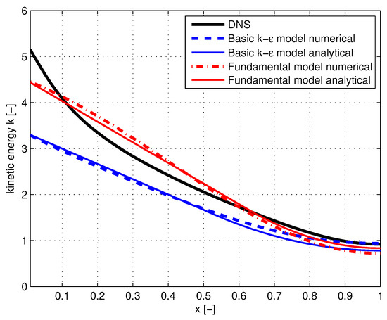
Figure 4.
Distribution of kinetic energy, k, versus x, according to DNS (solid line), the numerically and analytically assessed basic k- model (dashed and full lines, respectively), and the numerically and analytically assessed fundamental model (dash–dot and full lines, respectively).
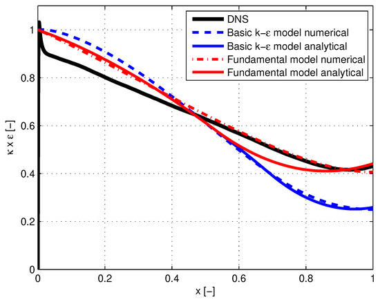
Figure 5.
Distribution of kinetic energy, G, versus x, according to DNS (solid line), the numerically and analytically assessed basic k- model (dashed and full lines, respectively), and the numerically and analytically assessed fundamental model (dash–dot and full lines, respectively).
6.3. Analytical Solution
The distinction is made between the area near the wall referred to as the outer region and the area near the center of the channel referred to as the inner region. The outer region is the area where the production and dissipation of energy are dominant. Turbulent diffusion of kinetic energy and pressure and turbulent diffusion of dissipation are negligibly small. It is the area where the log layer description for mean flow applies and where production equals dissipation [21]. In the inner region, turbulent diffusion of kinetic energy and pressure, as well as turbulent diffusion of dissipation, are important and in balance with energy dissipation, while production is negligibly small. For each region, analytical solutions can be derived, which are subsequently matched to arrive at a complete solution.
6.3.1. Solutions for k and G in the Outer Region
Solutions valid in the outer region are obtained by retaining the second and third terms in Equations (28) and (33), yielding and , or in terms of k and
- Basic k-ϵ model:
- Fundamental model:
- Fundamental model:
To derive the equations for G, which are applicable in the outer region, the second and third terms of Equation (41) need to be taken into account (and replacing B with A in Equation (41), for the basic k- model). Noting that in the outer region and one obtains for G from Equation (30) using relation (17) and from Equation (35) using relation (40), the result:
- Basic k-ϵ model and fundamental model:
The above descriptions for k and G are rather simple. They compare well with the numerical results for values of x, up to about . At greater distances from the wall, they start to deviate and fail to meet the conditions of the zero slope at . To overcome this deficiency, solutions valid for the inner region are developed.
6.3.2. Solutions for k in the Inner Region
Solutions for k are developed by describing k by a series of successive powers of . The linear term in is omitted in order to satisfy the zero-slope condition at . Disregarding terms of and higher, we write the following for k:
where is the value of k at ; and and a are to be determined. Substituting expression (47) in Equations (29) and (34), and equating the leading terms of for a in the basic k- and fundamental models, respectively, we obtain the following relations:
and
where is the value of G at . In deriving result (49), we take for at the value in accordance with Equation (37). The boundary between the inner and outer region is defined by . At this boundary, the value of k and its slope should match the values of the outer region. This yields the following relations:
for basic k- and the fundamental model, respectively. From Equations (47)–(51), the following solutions are obtained:
- For the basic k- model:
- and for the fundamental model:
6.3.3. Solutions for G in the Inner Region
For G in the inner region, the following expansion is used:
where the linear term, , is introduced to satisfy the boundary condition at : cf. Equations (33) and (39). The values of and a are to be determined. Substituting description (54) into Equations (30) and (35) and equating the leading terms of yield the following:
where
and
for the basic k- model and fundamental model, respectively. At the boundary of the inner and outer regions, , the values of G and its slope, according to the outer and inner regions, should become equal. This yields the following relations:
Eliminating from the above equations yields the following irreducible equation for :
The value of follows from Equation (56) by using the system’s values for the various parameters and taking for the value of the numerical calculations, i.e., . Consequently, and for the basic k- model and the fundamental model, respectively. Iteratively, one finds from Equation (60) that for the basic k- model and the fundamental model, . A complete analytical description of G for the outer and inner regions is obtained from Equation (46) when and Equations (54)–(56) when . The results are shown in Figure 5 with solid blue and red lines.
6.4. Discussion of Results
Numerical and analytical solutions for kinetic energy, k, and energy dissipation, , with the latter in terms of , have been developed for the basic k- model and a new fundamental model. The solutions are compared with DNS results and are shown in Figure 4 and Figure 5. Our conclusions are as follows:
- Analytical solutions agree in a satisfactory manner with numerical solutions. The analytical solutions reveal the relative contributions of turbulent diffusion, energy production, and energy dissipation in the outer and inner regions of the channel. They show to what extent the descriptions are empirically or fundamentally based and depend on calibration factors.
- Solutions for k in the outer region according to the fundamental model do not depend on calibration constants. They have a fundamental basis. The differences with DNS can be ascribed to errors as a result of truncation in the expansion with respect to , which underlies the fundamental model.
- Solutions for k in the inner region according to the fundamental model depend on the calibration factor, .
- Solutions for k in both the outer and inner regions, according to the basic k- model, depend on the calibration factors and .
- Solutions for G in the outer region, according to the fundamental model and the basic k- model, and , do not depend on calibration factors. Differences with DNS are due to some deviation between the value of production and dissipation in this area.
- Solutions for G in the inner region, according to the fundamental model and the basic k- model, and , respectively, depend on the calibration factors and .
- Using standard calibration constants in the solutions of the basic k- model results in notable deviations compared to DNS data. The deviations can be reduced by recalibrating , and . Deviations between diffusion constants remain significant because of different functional dependencies; see Figure 1, Figure 2 and Figure 3.
7. Velocity Distributions
The basic k- model is based on the assumption of an isotropic turbulence field. It cannot predict the anisotropic behavior of covariances or turbulent stresses. For the fundamental model, the distribution of follows from the solution of Equation (34). According to Equation (24b) , while , where k is given by Equation (37). In Figure 6, the distribution, versus x, of the calculated values of the standard deviations of the fluctuations , , and , is shown, according to the fundamental model and the results of DNS. Deviations are similar to those shown in [9] and are ascribed to the truncation of the expansions of , underlying the theory of the fundamental model. Deviations of the three variances, from k, which describe anisotropy, are next to the leading order in the expansion (cf. Equations (24a)–(24c)), and are, therefore, more sensitive to the truncation error.
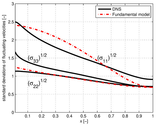
Figure 6.
Distribution of the standard deviations of fluctuating velocities , , and , versus x, according to DNS (solid line) and the fundamental model (dash–dot line).
For the gradient of the mean flow, the following relations can be derived. For the basic k- model from Equations (21) and (23b), we have the following:
For the fundamental model from Equations (21) and (24d), we have the following:
In Figure 7, the distributions are shown of versus x, according to DNS, the basic k- model, and the fundamental model. The deviations between DNS and the basic k- model are similar to those shown for and in Figure 1 and Figure 2. Similarly, the agreement between and is shown in Figure 1 and Figure 2. According to (21), , indicating that the disagreement of production with DNS in the case of the basic k- model is similar to that shown in Figure 7, and that the agreement of production with DNS for the fundamental model is similar to that shown in Figure 7.
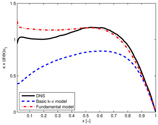
Figure 7.
Distribution of , versus x, according to DNS (solid line), the basic k- model (dash–dot line), and the fundamental model (dashed line).
The distribution of mean velocity predicted by the basic k- model and the fundamental model is obtained by integrating the RHSs of Equations (61) and (62). Because the models do not describe the velocity in the viscous layer at the wall, the integration starts at some distance from the wall for which the position is taken. The value of at this point, according to the DNS results of , is 17.2, which agrees with the values obtained from the measurements; see Monin and Yaglom, Vol. I, Figure 25 [21]. The results of the integration are shown in Figure 8, where the distributions of the mean velocity of the two models and DNS are presented. It is seen that for equal shear velocity (i.e., for equal longitudinal pressure gradient in the channel), the fundamental model somewhat overestimates mean velocity (by ), while the basic k- model underestimates it by .
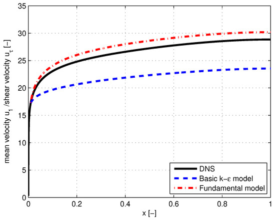
Figure 8.
Distribution of mean velocity divided by shear velocity, versus x, according to DNS (solid line), the basic k- model (dash–dot line), and the fundamental model (dashed line).
8. Discussion
An analysis is presented of two models to determine the mean values of turbulent flow variables, i.e., velocity, , pressure, p, turbulent diffusion, , kinetic energy, k, and energy dissipation, . The two models are the basic k- model widely used in engineering applications and environmental analysis [5,6], as well as a new fundamentally based model, which is derived from recently published statistical descriptions of inhomogeneous anisotropic turbulence [7,8,9]. The analysis focused on turbulent channel flow, which is highly anisotropic and inhomogeneous. It is of direct relevance to duct flow applications, turbulent boundary layers around bodies, and the atmospheric surface layer around the earth. Model predictions were verified against the published results of direct numerical simulations (DNS) for shear Reynolds numbers of 950 [15], 2000 [13], and [14]. The comparison focused on the regions outside the thin viscous boundary layers, which are a few millimeters at the wall. The development status of DNS is mature; its results can serve as a reliable source for verifying model predictions.
The basic k- model is built on an empirical isentropic representation of the turbulence field. It contains a gradient hypothesis for turbulent diffusion, which is supplemented by calibration constants. Using conventionally proposed values for the calibration constants [5,6], model predictions of several variables are found to deviate remarkably from the results of DNS. A summary is presented in Table 1.

Table 1.
The predictions of the basic k- model and the new fundamental model, compared with the DNS of turbulent channel flow.
The fundamental model is derived from a theory that has a theoretical basis [7,8,9]. Expressions for the turbulent diffusion of momentum and of conservative scalars, such as temperature and passive admixture (smoke, aerosols), are of a general nature. They are free from calibration constants. They are found to agree in a satisfactory manner with DNS results at all distances, x, from the wall (outside the thin boundary layer at the wall). The theory underlying the fundamental model does not provide generally valid expressions for the turbulent diffusion of non-conservative scalar kinetic energy, pressure, and energy dissipation. The non-conservative diffusion terms are only important for the determination of k and in the inner half of the channel. Here, non-conservative behavior has been modeled by using the diffusion expressions of conservative scalars provided with calibration factors. A summary is presented in Table 1.
9. Conclusions
CFD codes are generally based on empirical propositions for diffusion by turbulent fluctuations. This includes the basic k- model widely used in engineering and environmental analyses. The limitation of these models is that they lack generality. It is uncertain whether the constituting variables are truly and accurately represented by the proposed expressions, both in magnitude and spatial dependency. The addition of calibration factors tempers the prediction inaccuracies to some extent. At the same time, they need to be specified for each new case. However, calibration predictions can still deviate markedly from the correct results at different positions in the flow field.
Models that are derived from generally valid principles do not suffer from these limitations. The presented new model contains descriptions of important diffusion terms, which satisfy this criterion. Calibration factors are absent, and because of their generality, applicability exceeds that of channel flow. Points for improvement of the new model are as follows:
- (i)
- The agreements between the new model and DNS are satisfactory but not perfect, due to the truncation of the expansion in powers of the inverse of the universal Kolmogorov constant that underpins the theoretical foundation of the model. Extending the expansion will reduce the truncation error significantly.
- (ii)
- What is missing is a general description of the turbulent dispersion of non-conservative scalars. Their impact is limited to the description of k and in the interior part of the channel, or more generally, substantially away from walls where shear is imposed. The development of well-based descriptions for the diffusion of k and will eliminate the remaining empiricism of the model.
Funding
This research received no external funding.
Data Availability Statement
Data are contained within the article.
Acknowledgments
B.G.J. Ruis and H.S. Janssen are acknowledged for performing numerical calculations; G.M. Janssen is acknowledged for preparing the manuscript.
Conflicts of Interest
The author declares no conflicts of interest.
References
- Boussinesq, J. Mem.pres.par.div. savantis a l’acad. Sci. de Paris 1877, 24, 726–736. [Google Scholar]
- Taylor, G.I. Eddy Motion in the Atmosphere. Phil. Trans. R. Soc. Lond. A 1915, 215, 1–26. [Google Scholar] [CrossRef]
- Prandtl, L. 7. Bericht über Untersuchungen zur ausgebildeten Turbulenz. ZAMM 1925, 5, 136–139. [Google Scholar] [CrossRef]
- Von Kármán, T. Mechanische Ähnlichkeit und Turbulenz; Weidmannsche Buchh.: Berlin, Germany, 1930; pp. 58–76. [Google Scholar]
- Hanjalić, K.; Launder, B. Modelling Turbulence in Engineering and the Environment: Second-Moment Routes to Closure; Cambridge University Press: Cambridge, UK, 2011. [Google Scholar]
- Bernard, P.S.; Wallace, J.K. Turbulent Flow: Analysis, Measurement and Prediction; Wiley: Hoboken, NJ, USA, 2002. [Google Scholar]
- Brouwers, J.J.H. Statistical description of turbulent dispersion. Phys. Rev. E Stat. Nonlinear Soft Matter Phys. 2012, 86, 066309. [Google Scholar] [CrossRef] [PubMed]
- Brouwers, J.J.H. Statistical Models of Large Scale Turbulent Flow. Flow Turbul. Combust. 2016, 97, 369–399. [Google Scholar] [CrossRef][Green Version]
- Brouwers, J.J.H. Statistical Descriptions of Inhomogeneous fundamentally based Turbulence. Mathematics 2022, 10, 4619. [Google Scholar] [CrossRef]
- Monin, A.S.; Yaglom, A.M. Statistical Fluid Mechanics, Vol. II, Ch 8; Dover: New York, NY, USA, 2007. [Google Scholar]
- van Kampen, N.G. Stochastic Processes in Physics and Chemistry, 3rd ed.; Elsevier: New York, NY, USA, 2007. [Google Scholar]
- Stratonovich, R.L. Topics in the Theory of Random Noise; Gordon and Breach: New York, NY, USA, 1967; Volume 1. [Google Scholar]
- Hoyas, S.; Jiménez, J. Scaling of the velocity fluctuations in turbulent channels up to Re_τ = 2003. Phys. Fluids 2006, 18, 011702. [Google Scholar] [CrossRef]
- Hoyas, S.; Oberlack, M.; Alcántara-Ávila, F.; Kraheberger, S.V.; Laux, J. Wall turbulence at high friction Reynolds numbers. Phys. Rev. Fluids 2022, 7, 014602. [Google Scholar] [CrossRef]
- Kuerten, J.; Brouwers, J.J.H. Lagrangian statistics of turbulent channel flow at Re_τ = 950 calculated with direct numerical simulation and Langevin models. Phys. Fluids 2013, 25, 105108. [Google Scholar] [CrossRef]
- Kolmogorov, A. The Local Structure of Turbulence in Incompressible Viscous Fluid for Very Large Reynolds’ Numbers. Akad. Nauk. Sssr Dokl. 1941, 30, 301–305. [Google Scholar]
- George, W.K. The Decay of Homogeneous Isotropic Turbulence. Phys. Fluids A 1992, 4, 1492–1509. [Google Scholar] [CrossRef]
- Brouwers, J.J.H. Dissipation equals Production in the Log Layer of Wall Induced Turbulence. Phys. Fluids 2007, 19, 101702. [Google Scholar] [CrossRef]
- Lew, A.J.; Gustavo, C.; Carrica, B.; Carrida, P.M. A Note on the Numerical Treatment of the k-epsilon Turbulence Model*. Int. J. Comput. Fluid Dyn. 2001, 14, 201–209. [Google Scholar] [CrossRef]
- Borse, G.J. Numerical Methods with Matlab; Chapter 22; PWS Publishing: Boston, MA, USA, 1997; ISBN 0534938221. [Google Scholar]
- Monin, A.S.; Yaglom, A.M. Statistical Fluid Mechanics, Vol. I; Dover: New York, NY, USA, 2007. [Google Scholar]


Disclaimer/Publisher’s Note: The statements, opinions and data contained in all publications are solely those of the individual author(s) and contributor(s) and not of MDPI and/or the editor(s). MDPI and/or the editor(s) disclaim responsibility for any injury to people or property resulting from any ideas, methods, instructions or products referred to in the content. |
© 2024 by the author. Licensee MDPI, Basel, Switzerland. This article is an open access article distributed under the terms and conditions of the Creative Commons Attribution (CC BY) license (https://creativecommons.org/licenses/by/4.0/).