The Expected Dynamics for the Extreme Wind and Wave Conditions at the Mouths of the Danube River in Connection with the Navigation Hazards

Abstract

The entrance in the Sulina channel in the Black Sea is the target area of this study. This represents the southern gate of the seventh Pan-European transport corridor, and it is usually subjected to high navigation traffic. The main objective of the work is to provide a more comprehensive picture concerning the past and future expected dynamics of the environmental matrix in this coastal area, including especially the extreme wind and wave conditions in connection with the possible navigation risks. The methodology considered assumes analyses performed at three different levels. First, an analysis of some in situ measurements at the zero-kilometer point of the Danube is carried out for the 15-year period of 2009–2023. Together with the maximum wind speed and the maximum value of the wind gusts, the water level variation was analyzed at this point. As a second step, the analysis is based on wind speed data provided by regional climate models. Two periods, each spanning 30 years, are considered. These are the recent past (1976–2005), when comparisons with ERA5 reanalysis data were also performed, and the near future (2041–2070), when two different models and three climate scenarios were considered. The focus was on the extreme wind speed values, performing comparisons between the past and future expected extreme winds. Finally, the third analysis is related to the wave conditions. Thus, using as a forcing factor each of the wind fields that was previously analyzed, simulations employing a spectral wave model were carried out. The wave modeling system was focused using three different computational domains with increasing resolution towards the target area, and the nearshore wave conditions were evaluated. The results show that both the extreme wind and wave conditions are expected to slightly increase in the future. Especially in the wintertime, strong wind fields are often expected in this area, with wind gusts exceeding more than 70% of the hourly average wind velocity. With regard to the waves, due to the complex nearshore phenomena, considerable enhancements in terms of significant wave heights are induced, and there is also an elevated risk of the occurrence of rogue waves. This work is still ongoing, and taking into account the high navigation risks highlighted, the next step would be to elaborate the risk assessment of severe shipping conditions, particularly related to the likelihood or probability of adverse conditions with the potential of generating hazardous situations in this coastal environment.

1. Introduction

The dynamics of the last decades indicate that climate changes affect most natural systems in a significant way, and this especially concerns the global warming phenomena associated with higher temperature variations [1]. Furthermore, various climate scenarios (see, for example, [2,3]) indicate that a negative impact of climate change is expected in almost all regions of the world, inducing a visible enhancement in the intensity and frequency of the extreme events [4]. Coastal environments are more sensitive to such extreme events [5]. They represent the interface between land and water. On the other hand, the wind is usually stronger in the marine environment [6]. That is why its impact on the land located in the vicinity of the sea is usually higher.

The objective of the present work is to provide a more comprehensive picture concerning the expected dynamics of the extreme wind and wave conditions at the mouths of the Danube River in the Black Sea in connection with the navigation hazards. The focus is on the entrance to the Sulina channel, which represents the main navigation exit from the Danube to the Black Sea [7], being at the same time the southern gate of the seventh Pan-European transportation corridor linking the Black Sea to the North Sea via the Rhine-Main–Danube navigation system (inaugurated in 1992) [8]. The location of the target area in the Black Sea is illustrated in Figure 1. Since this represents the main southern entrance to the largest European inland navigation system, it is subjected to high navigation traffic [9]. Furthermore, for a distance of about 170 km, from Sulina at the Black Sea (considered the zero-kilometer point of the Danube) and up to the Romanian port of Braila (kilometer 170), the so-called Maritime Danube extends. The Danube is also navigable by maritime ships [10], while river ships can navigate upstream to Ulm in Germany [11]. Moreover, since the beginning of the war in Ukraine in February 2022, this traffic was significantly increased [12], with the Danube being an alternative and more secure route for the cereals and other goods exported by Ukraine.

The Danube also represents the most important water resource for the Black Sea [13], and the river outflow generates relatively strong currents in the coastal environment neighboring the deltaic zone. The Danube Delta, which is the largest in Europe [14], is delimited by the three principal branches of the river, Chilia, Sulina, and Saint George [15]. In this area, especially in spring, there are often risks of floods [16,17]. The wind and wave climate are characterized by relatively high-energy conditions [18], and extreme storms also occur with a certain frequency in this nearshore [19]. Furthermore, the waves are often increased at the mouths of the Danube by the wave–current interactions that occur between the incoming waves and the coastal currents induced by the river discharge into the sea [20]. Taking into account the complexity of this coastal environment and the associated processes [21], the relatively high frequency of severe weather conditions, the high navigation traffic, and the proximity of an ongoing war, various studies (see, for example, [22]) indicate that this area is subjected to high risks from the point of view of navigation hazards.

In this context, an analysis of the characteristics of the environmental matrix and its expected dynamics in the coastal area at the mouths of the Danube River, and especially at the entrance to the Sulina channel, is made in the present work. This analysis includes some in situ measurements for the wind and water level, reanalysis of wind data from the European Centre for Medium-Range Weather Forecasts (ECMWF), and projections of the future expected wind fields provided by regional climate models (RCMs) under various RCP (representative concentration pathway) and SSP (shared socioeconomic pathway) scenarios. Furthermore, an analysis of the wave conditions is also made by performing simulations over the entire basin of the sea using the SWAN (acronym from Simulating WAves Nearshore) spectral model [23] and focusing the modeling system with higher-resolution domains on the coastal environment at the mouths of the Danube River.

The present work can be considered as both actual and important because it provides reliable information concerning the navigation conditions and the associated risks in a coastal area with a high strategic and economic importance. At the same time, the proposed work has many elements of novelty. Thus, together with the past wind and wave conditions, the future expected wind and wave climate is assessed considering various climate models and scenarios. Another element of novelty is related to the probabilistic evaluation of the conditions when, due to the wave–current interactions, rogue waves may occur at the mouths of the Danube River.

2. Materials and Methods

2.1. In Situ Measurements

The bathymetric map of the target area considered in the present study is illustrated in Figure 2. Based on the information presented in references [24,25,26], the average currents generated by the Danube River outflow in the Black Sea are also represented on the map. Two types of data were available for the analysis, which was performed for the 15-year time interval of 2009–2023.

The first parameter analyzed is the water level. These values resulted from daily measurements [12] at the entrance to the Sulina channel. The water level is considered as the elevation of the free surface of the Danube relative to a specified vertical datum and refers to the difference in centimeters between the sampling point’ vertical datum in reference to a standard Black Sea elevation datum. The wind measurements, with data provided by reference [27], represent the second parameter analyzed. This includes the wind speed provided with a one-hour time step and the corresponding maximum speed of the wind gusts. The average wind direction is also provided by the data analyzed. Both the water level and wind measurements correspond to the zero-kilometer point of the Danube, denoted in Figure 2 as RP0 (reference point zero).

2.2. Wind Model Data Considered

The next analysis is based on the data coming from the wind models. These are carried out in two different locations, reference point 1 (RP1), which is offshore the Sulina channel with the coordinates (30.18° E, 45.12° N), and reference point 2 (RP2), which is offshore the Saint George arm of the Danube with the coordinates (30.01° E, 44.82° N). The first analysis of the wind climate relates to the hindcast period of 30 years (the interval of 1976–2005). The ERA5 database is considered for this analysis. This is a relatively new reanalysis wind product, being an upgrade of the former ERA-Interim [28]. These data start in 1950 and end five days behind the current time. They are provided in the public domain by the European Centre for Medium-Range Weather Forecasts, which is the most recent and one of the most reliable global atmospheric reanalysis databases. The resolution of the ERA5 wind data is 0.25° × 0.25° in the geographical space, and the time step is one hour. For each hour, it gives wind and atmospheric pressure fields that are consistent with the previous evolution of the parameters modelled. In the present work, the wind speed at a 10 m height above the sea level is considered for the analysis, with a 3 h time step.

The second 30-year time period taken into account for analysis considering various climate scenarios (RCP4.5, RCP8.5, and SSP5-8.5) and atmospheric models is 2041–2070. The first wind field considered is that given by the regional climate atmospheric model version 4 (RCA4) provided by the Rossby Centre of the Swedish Meteorological and Hydrological Institute (SMHI) [29]. This regional climate model is driven by the global climate model (GCM), MPI-M-MPI-ESM-LR [30]. MPI-M means the Max Planck Institute for Meteorology, while MPI-ESM indicates the Max-Planck-Institute Earth System Model, and LR is low resolution. These data are made available in the public domain via the COPERNICUS database [31]. A second RCM considered is ALADIN (versions 6 for RCPs and 6x for SSP5-8.5) [32]. ALADIN stands for Aire Limitée Adaptation dynamique Développement International and is a regional climate model forced by the global atmospheric model GCM CNRM-CM5 (Centre National de Recherches Météorologiques), which is an Earth system model that is designed to run climate simulations. This GCM comprises the ARPEGE Climate Model [33]. ARPEGE is run by Météo-France and is the acronym from Action de Recherche Petite Echelle Grande Echelle, with the meaning of a research project on small and large scales. With regard to the SSP climate scenarios, the data considered come from the fully coupled regional climate system model CNRM-RCSM6/ALADIN [34,35] (where RCSM is the acronym for regional climate system model). In addition to the analysis of the data for the 30-year future time period (2041–2070), comparisons were performed with the ERA5 data for the past. Taking into account the availability of the data from the climate wind models, which is different for the SSP scenarios than the data for the RCP scenarios, the 30-year time interval (1979–2008) was considered for SSP, while for RCP (either 4.5 or 8.5) the initial 30-year time interval (1976–2005) was kept.

2.3. Wave Model Simulations

The third-generation phase-averaged model SWAN [23] is considered in the present work to predict the wave conditions. This was implemented and validated against satellite data and in situ measurements in the entire basin of the Black Sea, and further on, it was focused considering a higher-resolution domain on the coastal area at the mouths of the Danube. This wave model is based on the spectrum concept and solves an advection-type equation in five dimensions (time, geographical, and spectral spaces) [36,37]. As in most of the spectral wave models, the spectrum considered is the action density spectrum (N) and not the energy density spectrum. This is because in the presence of the currents, the action density is conserved while the energy density is not. The action density is equal to the energy density (E) divided by the relative frequency ($\sigma$). Although SWAN was initially designed mainly for the nearshore areas, during this time, the model was developed in a significant way, and now it can also be successfully used on sub-oceanic and even oceanic scales, having performances comparable with standard wave models such as WAM (Wave Model) [38] or WW3 (Wave Watch 3) [39], which are designed for large scales. With regard to the sub-oceanic scales, SWAN becomes one of the most appropriate models, since one single model can be focused from large-scale generation to high-resolution domains via various computational levels. From this perspective, SWAN may be considered at this moment to be the most effective and reliable numerical model for predicting wave conditions and climate in an enclosed sea basin such as the Black Sea [40].

The advection-type equation considered in the SWAN model has the following general expression:

$$\frac{\partial N}{\partial t}+\nabla \left(N\right)+\frac{\partial }{\partial \sigma }\dot{\sigma }N+\frac{\partial }{\partial \theta }\dot{\theta }N=\frac{S}{\sigma },$$

(1)

For larger-scale applications, the spherical coordinates, longitude $\left(\lambda \right)$, and latitude $\left(\phi \right)$ are considered, and the operator $(\nabla )$ has the following expression:

$${\nabla }_{\mathrm{S}\mathrm{p}\mathrm{h}}\left(N\right)=\frac{\partial }{\partial \lambda }\dot{\lambda }N+\frac{1}{\cos \phi }\frac{\partial }{\partial \phi }\dot{\phi }N,$$

(2)

For coastal applications, the Cartesian coordinates (x) and (y) are more appropriate, and in this case, the operator $(\nabla )$ becomes:

$${\nabla }_{\mathrm{C}\mathrm{a}\mathrm{r}\mathrm{t}}\left(N\right)=\frac{\partial }{\partial x}\dot{x}N+\frac{\partial }{\partial y}\dot{y}N,$$

(3)

The left side of Equation (1) represents the kinematic part, and it indicates the propagation of the wave action in time, geographical, and spectral spaces. Some relevant phenomena such as wave diffraction or refraction are also included. The source (S) is expressed on the right hand side as the energy density components. Three components are more relevant in deep water. They correspond to the atmospheric input, dissipation by whitecapping, and nonlinear quadruplet interactions. In shallow and intermediate water, additional terms are included. They correspond especially to the finite depth effects and comprise phenomena such as depth-induced wave breaking, bottom friction, or triad nonlinear wave–wave interactions. Thus, the expression of the source term is as follows:

$$S=S_{in}+S_{nl}+S_{diss}+S_{fd}$$

(4)

Such a SWAN-based wave prediction system was previously implemented in the basin of the Black Sea and focused on its western coast, considering various computational levels [41,42].

Table 1. Characteristics of the computational domains defined for the SWAN model simulations focused on the coastal area at the mouths of the Danube in the Black Sea.

Spherical Domains	Δλ × Δφ	Δt (min)	nf	nθ	ngλ × ngφ = np
Sph1—Black Sea	0.08° × 0.08°	10 non-stat	24	36	176 × 76 = 13,376
Sph2—Danube mouths	0.01° × 0.01°	10 non-stat	24	36	71 × 61 = 4331
Cartesian Domain	Δx ×Δy (m)	Δt (min)	nf	nθ	ngx × ngy = np
Cart—Sulina	50 × 50	60 stat	30	36	135 × 216 = 29,160

presents the characteristics of the three computational domains considered in the present work. The first domain, defined in spherical coordinates (longitude and latitude, Δλ and Δφ), corresponds to the entire basin of the Black Sea (illustrated in Figure 1 and Figure 2). The second computational domain, defined also in spherical coordinates, is focused on the coastal area at the mouths of the Danube River and the corresponding geographical space. This is illustrated in Figure 2. Finally, a higher-resolution domain focused only on the Sulina channel was defined in Cartesian coordinates. The corresponding geographical space is illustrated in Figure 1.

Table 1 indicates the resolution in the geographical space (Δλ and Δφ, measured in degrees for spherical coordinates and Δx and Δy, measured in meters for Cartesian coordinates), where Δt is the time resolution in minutes, nf is the number of frequencies considered in the spectral space, nθ is number of directions, ngλ (or ngx) is the number of grid points along the longitude (or x-axis), ngφ (or ngy) is the number of grid points along the latitude (or y-axis, respectively), and np is total number of grid points. As it is known, in the case of the structured grids, the computational domain corresponding to the geographical space is discretized with a constant spatial step. This may, however, be different between the x and y axes, or between the longitude and latitude for the case of the spherical coordinates. On the other hand, the spectral space is defined by the number of frequencies (nf) having a logarithmic distribution and the number of directions (nθ) that are equally distributed. This means that the directional step considered in these simulations is constant (Δθ = 10°), while the step in the frequency space (Δf) is variable. It must also be highlighted at this point that, in the case of the larger geographical spaces, the spherical coordinates and the non-stationary mode are more reliable, while for the high-resolution computational domains, the Cartesian coordinates and stationary mode are usually considered to be more effective.

The physical processes activated in the SWAN simulations, corresponding to each of the three computational domains considered in the present work are presented in

Table 2. Physical processes activated in the SWAN simulations, corresponding to the eight defined computational domains. X—process activated, 0—process inactivated.

Input/Process	Wave	Wind	Tide	Curr	Gen	Wcap	Quad	Triad	Diffr	Bfric	Set Up	Br
Domains
Sph1	0	X	0	0	X	X	X	0	0	X	0	X
Sph2	X	X	0	X	X	X	X	X	0	X	0	X
Cart	X	X	0	X	X	X	X	X	X	X	X	X

. In this table, Wave indicates the wave forcing, Wind indicates the wind forcing, Td indicates the tide forcing, Curr indicates the current field input, Gen indicates generation by wind, Wcap indicates the whitecapping process, Quad is the quadruplet nonlinear interactions (interactions between four waves that usually occur in deep water), Tri is the triad nonlinear interactions (reflecting the interactions between three waves, which are usually characteristic to intermediate and shallow water), Dif is the diffraction process, Bfr is the bottom friction, Set up is the wave-induced set up, and Br is the depth-induced wave breaking.

Previous calibrations and validations were carried out to assess the reliability and performance of this wave prediction system in the Black Sea, indicating that the SWAN results are in general reliable for both average energy and storm conditions. For example, in reference [43], comparisons against satellite data were performed for the 20-year period of 1997–2016. In terms of significant wave heights (Hs), the following values resulted for the main statistical parameters: Bias = 0.05 m, RMSE = 0.38 m, SI = 0.36, R = 0.87, and S = 0.99. The parameters above presented are Bias, root mean square error (RMSE), scatter index (SI), correlation coefficient (R), and the regression slope (S), all of them being computed according to their standard definitions, as given below, where X_i represents the measured value, Y_i is the simulated value, and n is the number of observations:

$$X_{med}=\tilde{X}=\frac{\sum _{i=1}^n{X}_i}{n}, Bias=\frac{\sum _{i=1}^n\left(X_i-Y_i\right)}{n}, RMSE=\sqrt{\frac{\sum _{i=1}^n{\left(X_i-Y_i\right)}^2}{n}}$$

(5)

$$SI=\frac{RMSE}{\tilde{X}}, r=\frac{\sum _{i=1}^n\left(X_i-\tilde{X}\right)\left(Y_i-\tilde{Y}\right)}{{\left(\sum _{i=1}^n{\left(X_i-\tilde{X}\right)}^2\sum _{i=1}^n{\left(Y_i-\tilde{Y}\right)}^2\right)}^{\frac{1}{2}}}, S=\sqrt{\frac{\sum _{i=1}^n{Y_i}^2}{\sum _{i=1}^n{X_i}^2}}$$

(6)

It has to be highlighted at this point that the values of the statistical parameters Bias, RMSE, and SI are better when they are smaller, while the correlation coefficient and the regression slope are considered to be better when they are closer to the unity. In the case of the waves with significant wave heights higher than 3 m (associated with the storm conditions), for the 20-year time interval considered, the following values resulted for the main statistical parameters: Bias = −0.07 m, RMSE = 0.47 m, SI = 0.21, R = 0.78, and S = 1.05. Furthermore, the simulation results also indicate that, in the Black Sea basin, the storm waves represent about 2% of the total. These statistical results can be considered as reasonably accurate, and they give a good degree of credibility to the analyses related to the past and future storm conditions in the Black Sea, which are presented next. Furthermore, an assimilation scheme of the satellite data, based on an optimal interpolation approach, has been implemented [44], improving the statistical results in relative terms (Bias 57%, RMSE 17%, SI 20%, R 3%, and S 1%). It should also be highlighted that the above results were performed when the wave modeling system was forced with ERA5 reanalysis data, while for the future wave projections, RCM wind data have been used [45], considering SWAN version 41.31AB.

3. Results

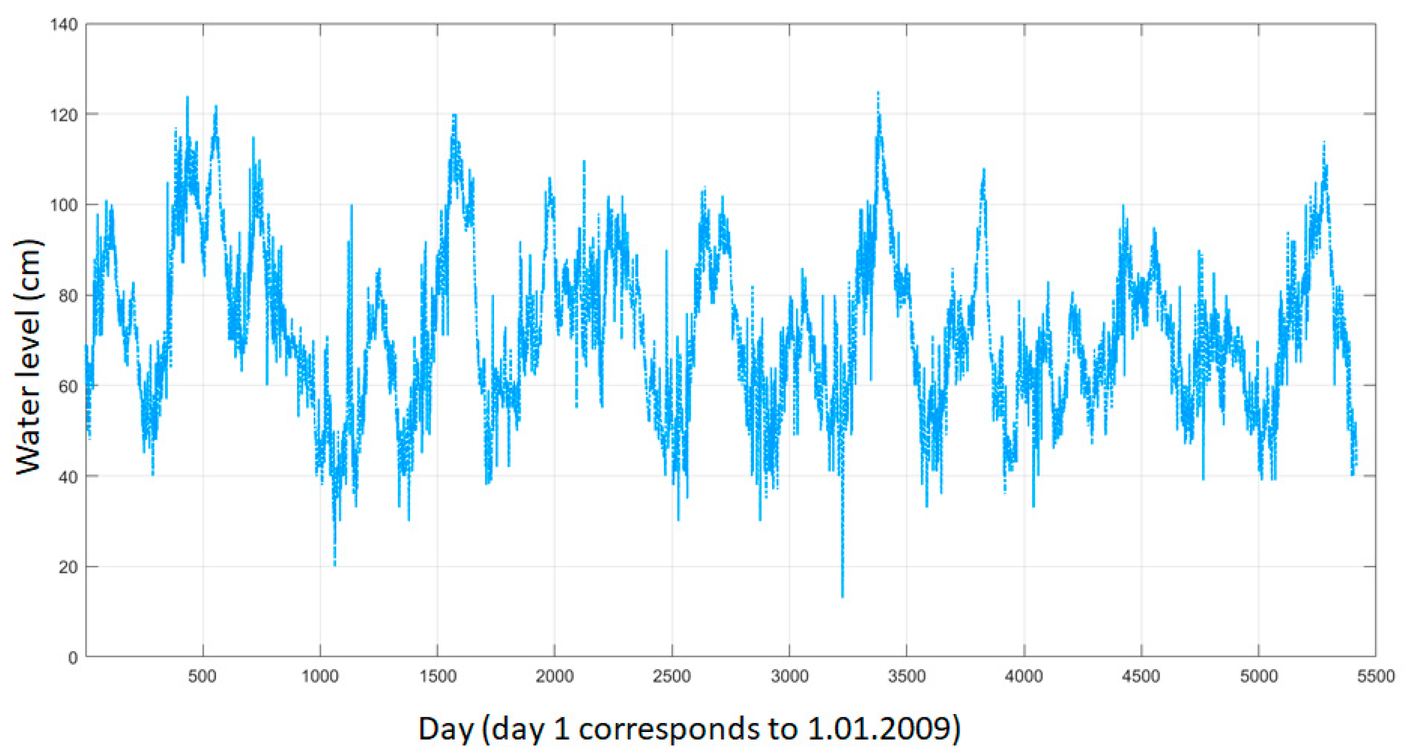
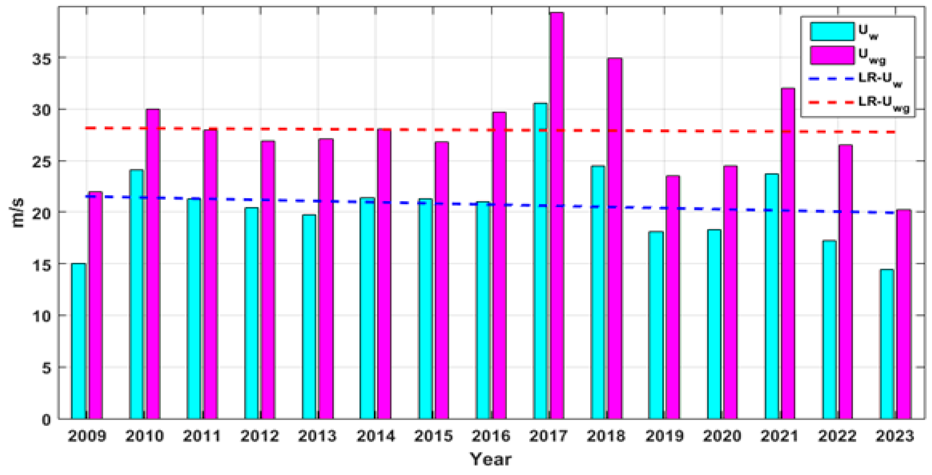
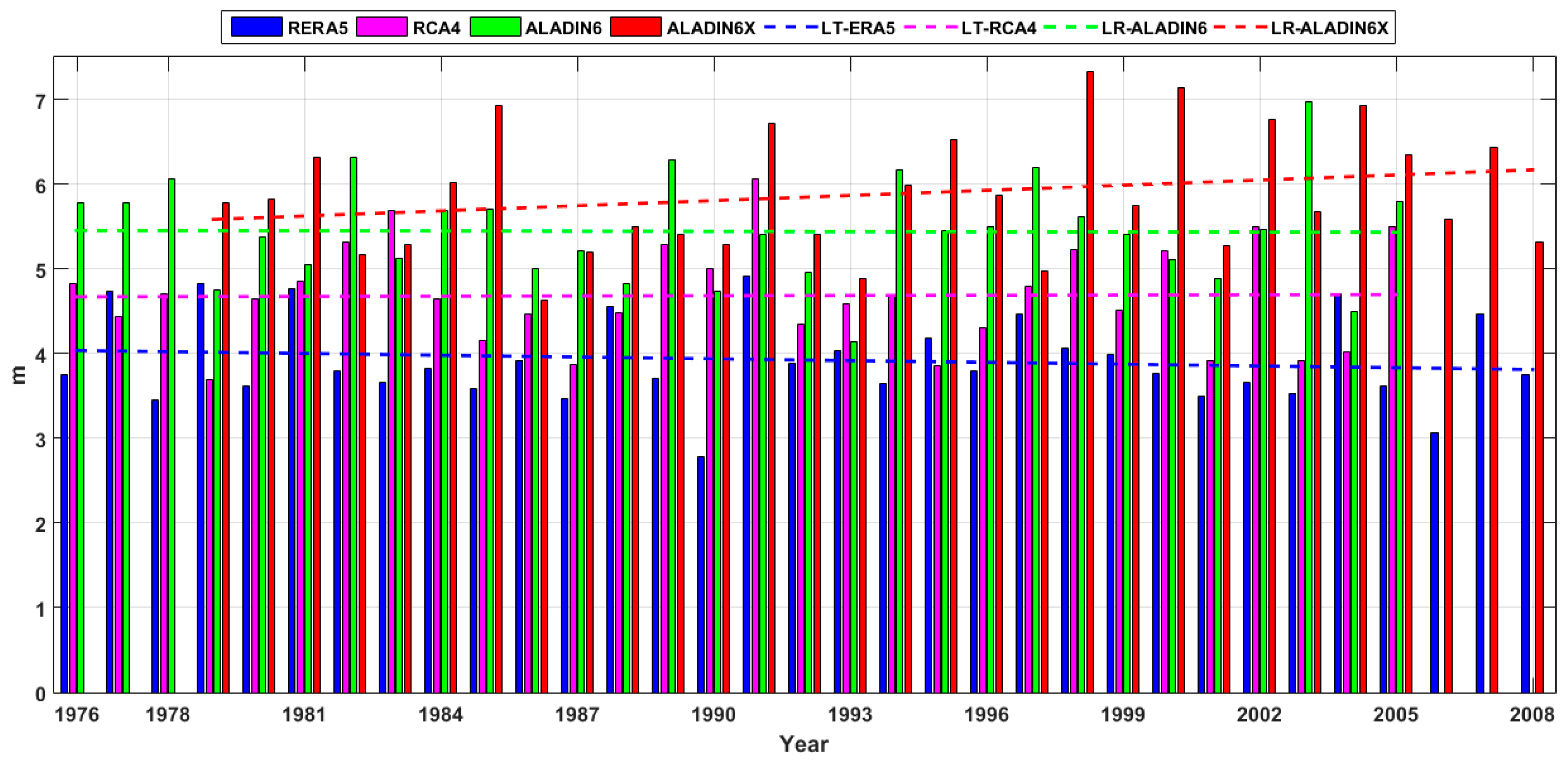
3.1. Analysis of the In Situ Measurements

An analysis of some in situ measurements performed at the entrance to the Sulina channel (denoted in Figure 1 as RP0) is performed next for the 15-year time interval of 2009–2023. The first parameter considered is the water level. Figure 3 illustrates the variations in the water level at the entrance to the Sulina channel (RP0). The data processed present the results of the daily measurements carried out for the 15-year time interval of 2009–2023. The results show that the maximum value of the water level measured during this time interval was 125 cm, the minimum was 13 cm, and the average value was 71.6 cm.

The next analysis relates the wind speed measured at the same reference point (RP0). The data processed provides the hourly values of the wind speed (Uw), the maximum value of the wind gust (Uwg) registered in the respective hour, and the mean wind direction. Thus, Figure 4 presents the wind roses for the two parameters, Uw and Uwg. Figure 5 illustrates the annual maximum series (bars) for both wind parameters considered (Uw and Uwg), corresponding to the 15-year time interval considered. In this figure, the linear regression (indicating the trend) is also illustrated. A trend line, or the line of best fit [46], is given by the following relationship:

y = sx + m,

(7)

where x is the independent variable, y is the dependent variable, s is the slope of the line, and m is the y-intercept. The regression parameters (s and m) are computed based on the following relationships:

$$s=\frac{\sum _{i=n}^n\left(x_i-\overline{x}\right)\left(y_i-\overline{y}\right)}{\sum _{i=1}^n{\left(x_i-\overline{x}\right)}^2}$$

(8)

$$m=\overline{y}-s\overline{x}$$

(9)

whith n the number of years for which the maximum annual values were calculated (in the present case, 15 years), x is the independent variable represented by each year and y is the dependent variable indicating the maximum value corresponding to each year.

Table 3. Maximum values for the wind speed (Uw) and wind gust (Uwg) corresponding to each month for the 15-year period of 2009–2023.

Month	Jan	Feb	Mar	Apr	May	Jun	Jul	Aug	Sep	Oct	Nov	Dec
Uw (m/s)	30.6	24.1	17.2	21.0	16.9	16.7	20.7	17.6	18.3	18.4	18.2	21.4
Uwg (m/s)	39.4	32.0	22.4	27.3	21.2	24.0	23.9	23.0	23.3	25.6	24.2	30.0
Uwg/Uw	1.29	1.33	1.30	1.30	1.25	1.44	1.16	1.31	1.27	1.39	1.33	1.40

presents the maximum values of the wind speed and wind gust, corresponding to each month for the 15-year period of 2009–2023. The values of the ratio between Uwg and Uw are also presented in this table. As can be seen in Table 3, the maximum value of this ratio is 1.44. However, it can be noticed that this value is mainly characteristic to the high winds, because the average value of the same ratio for the entire data set is 1.73. This means that under normal conditions, we can very often expect wind gusts with an intensity that is almost double than the hourly registered value of the wind speed at the entrance to the Sulina channel.

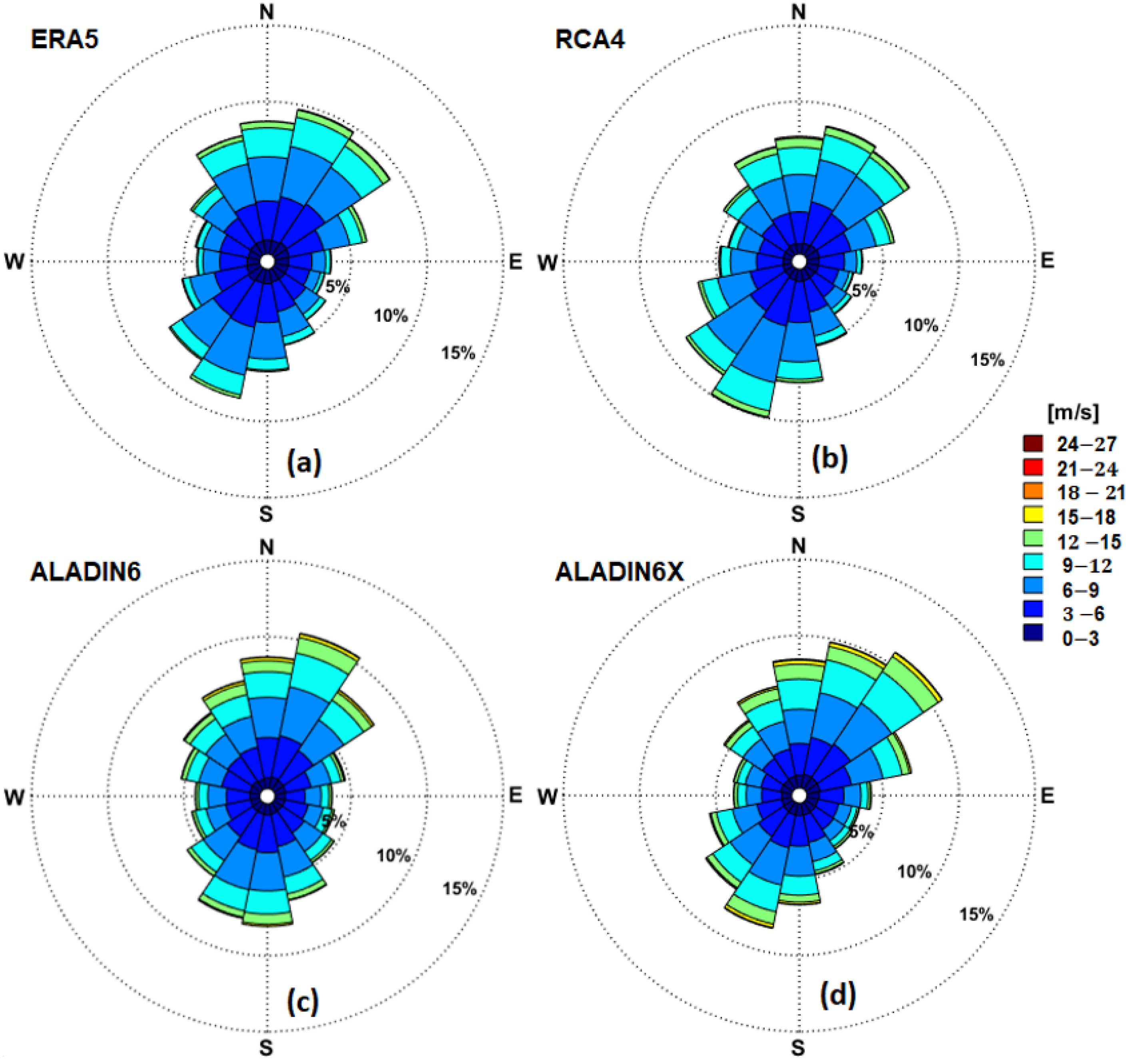
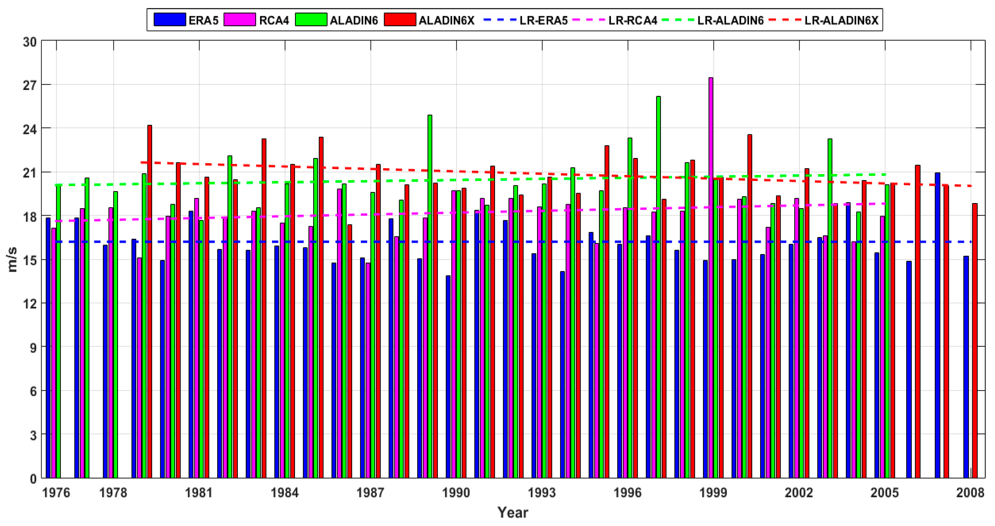
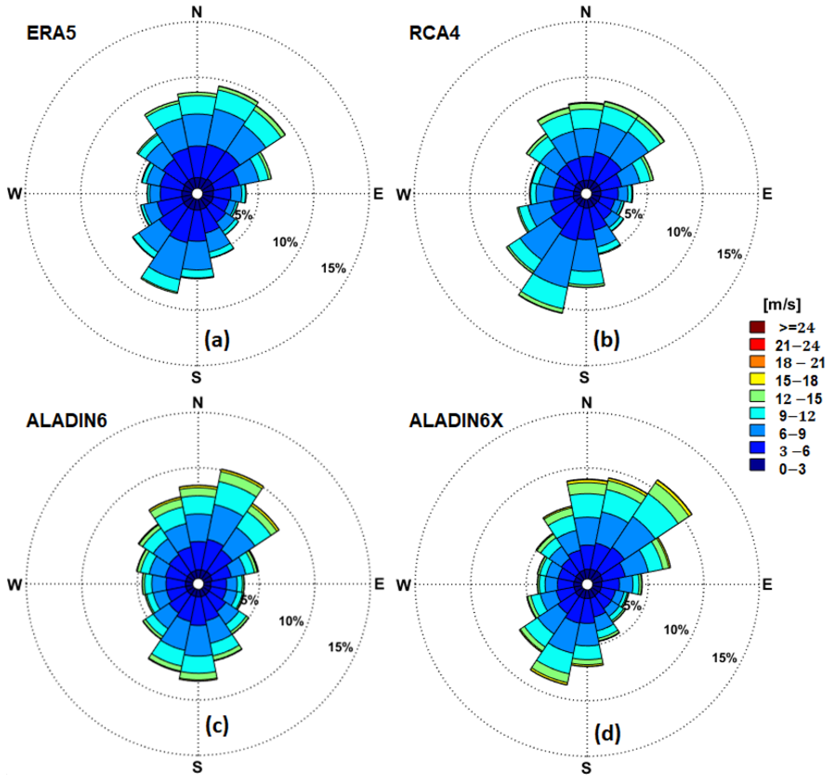
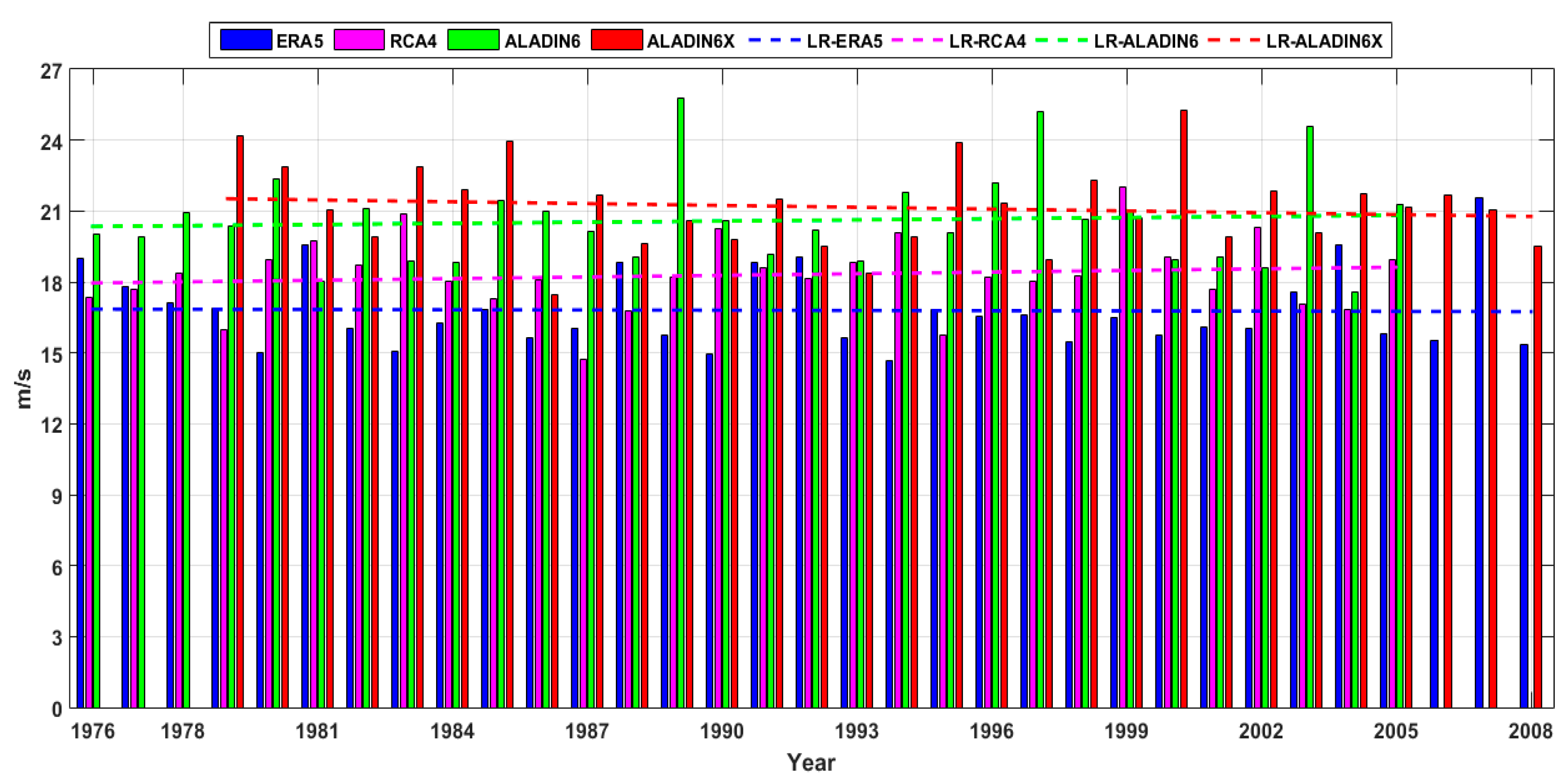
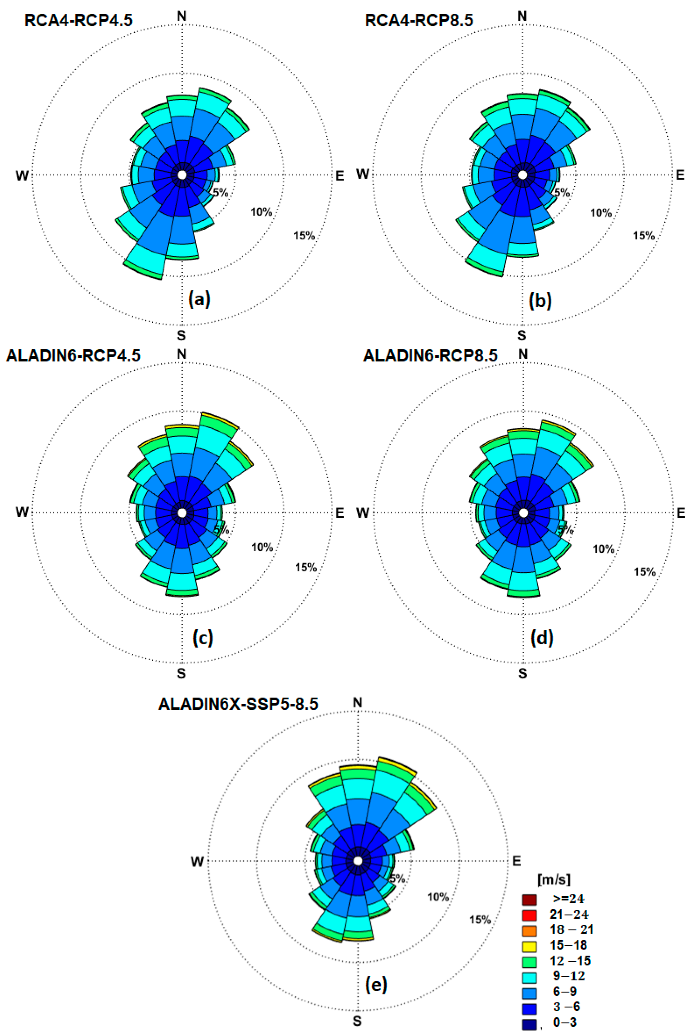
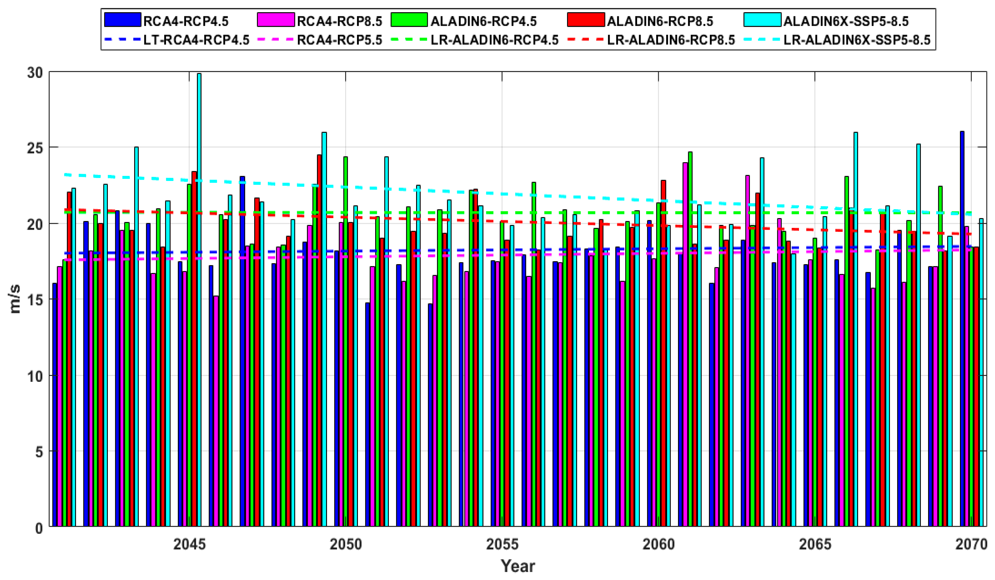
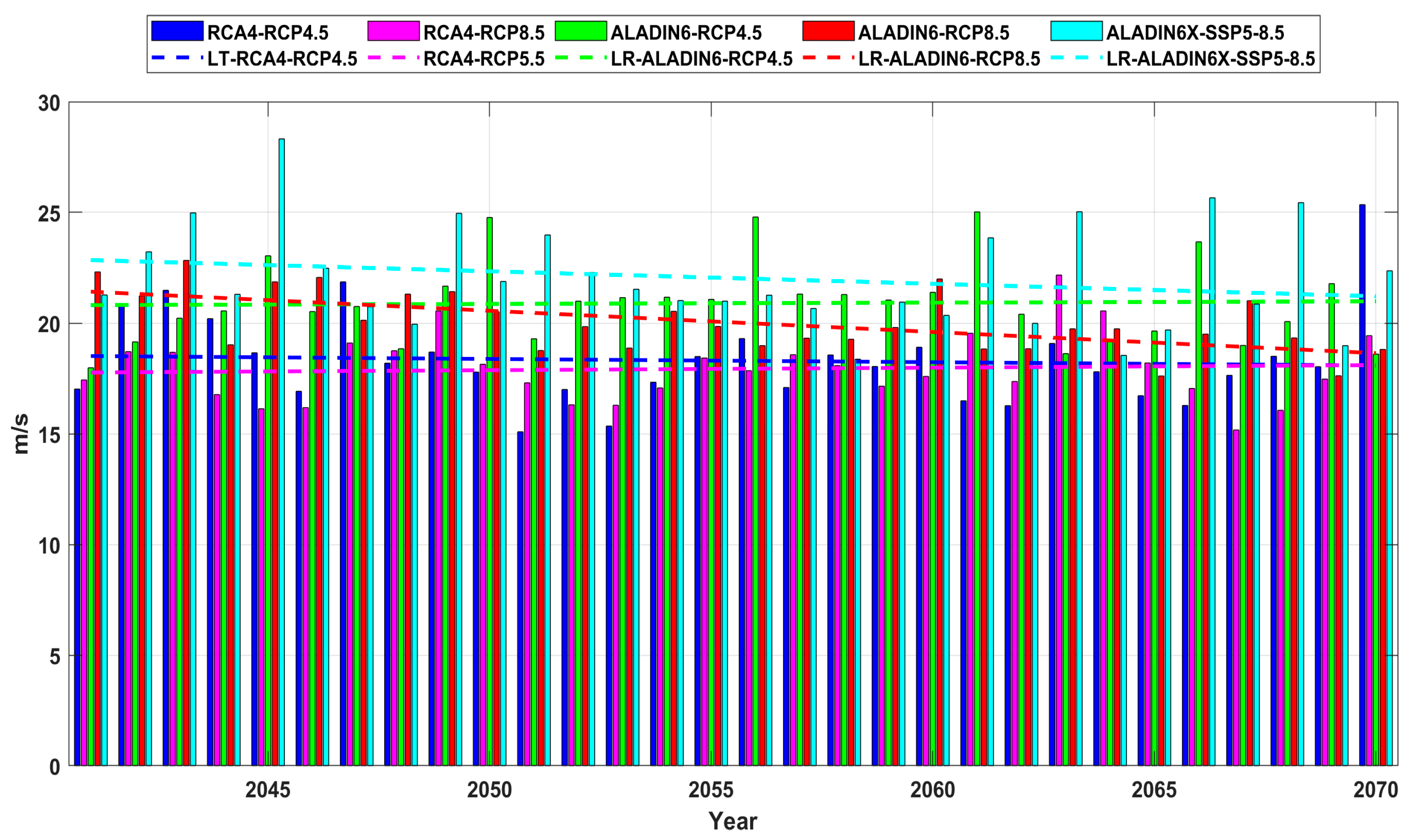
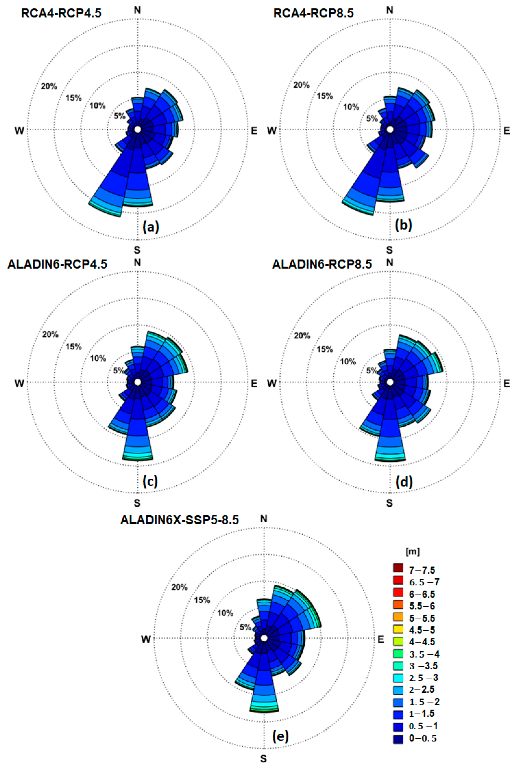
3.2. Analysis of Wind Data Offshore the Danube’s Mouths: Recent Past vs. near Future

The next analysis is made considering model wind data for the reference points RP1 (offshore Sulina) and RP2 (offshore Saint George). The analysis is made first for the past by processing the ERA5 data. The regional climate wind models, considered to evaluate the future expected wind conditions for the near future period of 2041–2071, are RCA4 and ALADIN6, both for RCP4.5 and RCP8.5, and ALADIN6x for SSP5-8.5. Since the historical data provided by the climate models are available for the 30-year time interval of 1976–2005, this period is considered for comparison with the ERA5 reanalysis data to assess the convergence and differences between the hindcast and historical data of the wind models. On the other hand, the SSP data are provided starting with 1979. In this case, the comparison with ERA5 is made for the 30-year period of 1979–2008. The wind roses corresponding to the reference points RP1 and RP2 (Sulina and Saint George, respectively) are illustrated in Figure 6 and Figure 7. In order to cover the entire period of 1976–2008, Figure 6a and Figure 7a were designed for this 33-year period, Figure 6b,c and Figure 7b,c for the 30-year period of 1976–2005, and Figure 6d and Figure 7d for the 30-year time interval of 1979–2008. First, it can be noticed from these figures that the wind conditions in the two locations (RP1 and RP2) are generally similar. With regard to the values of the maximum wind speed, for Sulina, they are U_10ERA = 20.94 m/s, U_10RCA = 27.49 m/s, U_10AL6 = 26.16 m/s, and U_10AL6x = 24.2 m/s, while for Saint George, they are U_10ERA = 21.55 m/s, U_10RCA = 22.01 m/s, U_10AL6 = 25.77 m/s, and U_10AL6x = 25.4 m/s. According to the results presented, the highest value of the maximum wind speed (27.49 m/s) between the two reference points considered corresponds to RP1 (Sulina). This was provided by the RCA4 climate wind model.

The annual maximum series corresponding to the same time intervals form the recent past considered before are presented in Figure 8 (for RP1) and Figure 9 (for RP2). At this point, it should be also highlighted that the time step of all the wind model data considered and processed is of 3 h, so considerably higher wind speed values can occur in this time window. It should be also noticed that there is an acceptable concordance between the models and the RCMs (especially ALADIN), providing generally higher wind speed values than ERA5.

The wind roses expected for the near future period (2041–2070) are illustrated in Figure 10 and Figure 11 for RP1 and RP2, respectively. The results presented indicate similarity with the recent past, with the observation that a higher percentage of the wind coming from the Northeast direction is expected in the future.

The corresponding annual maximum series and linear trends are presented in Figure 12 and Figure 13, respectively. For Sulina, the maximum values of the wind speed evaluated using the climatic models are U_10RCA4.5 = 26.11 m/s, U_10RCA8.5 = 23.96 m/s, U_10AL4.5 = 24.65 m/s, U_10AL8.5 = 24.48 m/s, and U_10AL5-8.5 = 29.85 m/s, while for Saint George, they are U_10RCA4.5 = 25.35 m/s, U_10RCA8.5 = 22.16m/s, U_10AL4.5 = 25.02 m/s, U_10AL8.5 = 22.83 m/s, and U_10AL5-8.5 = 28.32 m/s.

As for the recent past period, the results show that in the near future time interval considered, the highest wind speed is also expected in Sulina (29.85 m/s). However, this time, the highest wind conditions are provided by the SSP5-8.5 climate scenario.

It can also be noticed that, for the near future period analyzed, the SSP5-8.5 data provide systematically higher wind speed values than all the other climate scenarios. On the other hand, the SSP data indicate higher wind speeds than in the past, a relative increase of about 22% in RP1 and of 11.5% in RP2. From this perspective, the results indicate a slight tendency of enhancement of the extreme winds in the coastal environment at the mouths of the Danube River. This tendency has also been reported in other works (for example, reference [47]).

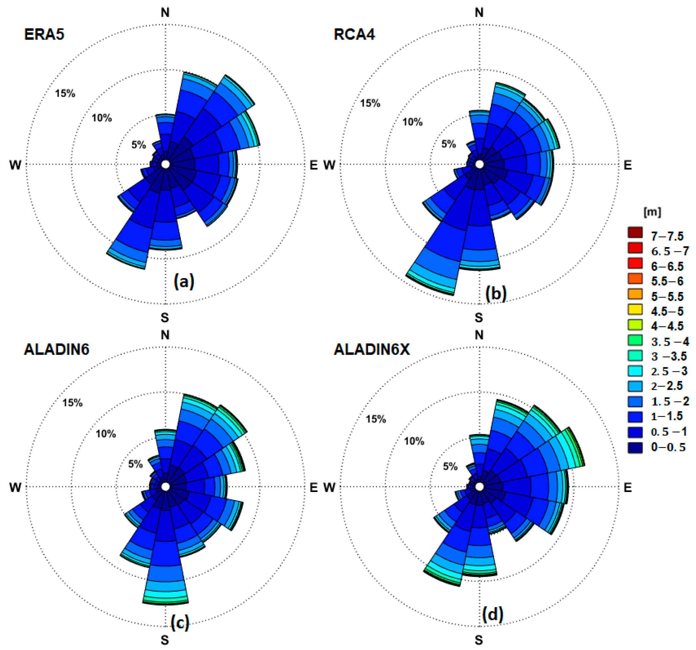
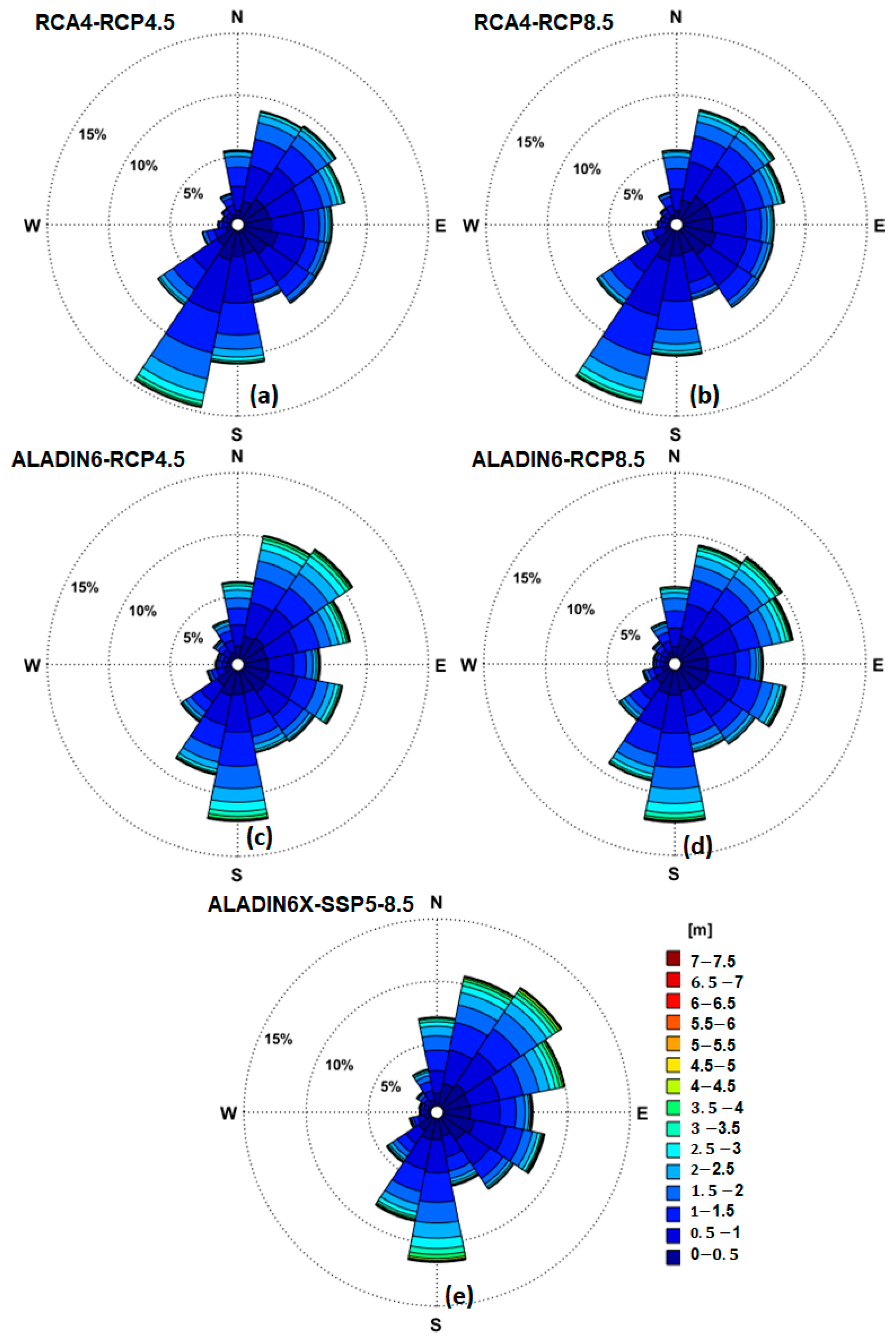
3.3. Analysis of Wave Data Offshore the Danube’s Mouths: Recent Past vs. near Future

Using the wind fields provided by ERA5 for the recent past and those coming from the regional climate models (RCA4 and ALADIN) under the scenarios previously considered (RCP4.5, RCP8.5 and SSP5-8.5), simulations employing the wave modeling system SWAN based were carried out. The focusing of the system towards the target area for a case of a typical storm in the Black Sea corresponding to the timeframe 21.12.2004h03 is illustrated in Figure 14 in terms of significant wave height scalar fields and wave vectors. The wave vectors indicate the mean wave direction, and their numerical values are represented by the value of the significant associated wave height. The color bar given in this figure associates a different color to each interval value of 0.5 m for the significant wave height. According to the results presented in this figure, for the case of the storms propagating from east to west (which are typical for this region), due to the effects of the wave-current interactions at the mouths of the Danube River, the significant wave height values are very high and very close to the higher value in the entire sea basin. For example, in Figure 14, the maximum Hs value in the Black Sea is 7.26 m, while the maximum Hs value at the mouths of the Danube is 7.24 m.

Based on the results of the wave modeling system in the two reference points defined RP1 and RP2 for the two 30-year time intervals (recent past and near future), and considering as forcing factors the wind fields provided by the models mentioned in the previous section, an analysis of the past and future expected wave climate in the target area is presented next.

The Hs wave roses corresponding to the reference points RP1 and RP2 (Sulina and Saint George, respectively) are illustrated in Figure 15 and Figure 16. In order to cover the entire period of 1976–2008, Figure 15a and Figure 16a were designed for this 33-year period, Figure 15b,c and Figure 16b,c for the 30-year period of 1976–2005, and Figure 16d and Figure 17d for the 30-year time interval of 1979–2008. As in the case of the wind, it can be noticed from these figures that the wave conditions in the two locations (RP1 and RP2) are in general similar in terms of both Hs and wave directions. With regard to the maximum Hs values, for Sulina, they are H_sERA = 4.5 m, H_sRCA = 5.65 m, H_sAL6 = 6.27 m/s, and H_sAL6x = 7.04 m, while for Saint George, the results are H_1s0ERA = 4.91 m, H_sRCA = 6.061 m, H_sAL6 = 6.96 m, and H_sAL6x = 7.33 m/s. According to the results presented, the highest value of the significant wave height (7.33 m/s) between the two reference points considered corresponds to RP2. This was provided by the ALADIN6x wind model as the forcing system for SWAN.

The annual maximum series corresponding to the same time intervals from the recent past considered before are presented in Figure 17 (for RP1) and Figure 18 (for RP2). It should be mentioned that, as in the case of the wind, the time step considered for the wave model output is 3 h. It should be also noticed that there is an acceptable concordance between the models. However, it can be observed at this point that when forcing the wave modeling system, the RCMs (and especially ALADIN) generally provide higher Hs values than ERA5.

The Hs wave roses expected for the near future period (2041–2070) are illustrated in Figure 19 and Figure 20 for RP1 and RP2, respectively. The results presented are similar to those from the recent past. The corresponding Hs annual maximum series and linear trends are presented in Figure 21 and Figure 22, respectively. For Sulina, the maximum Hs values evaluated are H_sRCA4.5 = 6.19 m, H_sRCA8.5 = 6.13 m, H_sAL4.5 = 7.13 m, H_1AL8.5 = 5.7 m, and H_sAL5-8.5 = 7.05 m, while for Saint George, they are H_sRCA4.5 = 6.86 m, H_sRCA8.5 = 6.51 m, H_sAL4.5 = 7.29 m, H_1AL8.5 = 6.19 m, and H_sAL5-8.5 = 7.31 m.

At this point, it can be noticed that, for the near future period analyzed, a similar tendency to the case of the wind fields occurs, in the sense that the ALADIN data provide higher values for the significant wave heights than when the RCA4 model is considered as the forcing wind field for the wave model. However, unlike in the case of the wind analysis, ALADIN6 for the RCP4.5 climate scenario provides higher Hs values in the target area than the SSP5-8.5 data. Finally, it can be also underlined that the results provided by the RCMs for the recent past in terms of the maximum values of the significant wave height, which may occur offshore the coastal area at the mouths of the Danube River, appear to be more realistic than the ones provided when ERA5 is considered as the wind driver for the wave model. This is probably because the ERA5 data have a tendency to systematically underestimate the maximum wind speed values. This observation is in line with the findings of various previous works (for example, references [43,44,45] or [47,48]), but also with some in situ observations.

4. Discussion

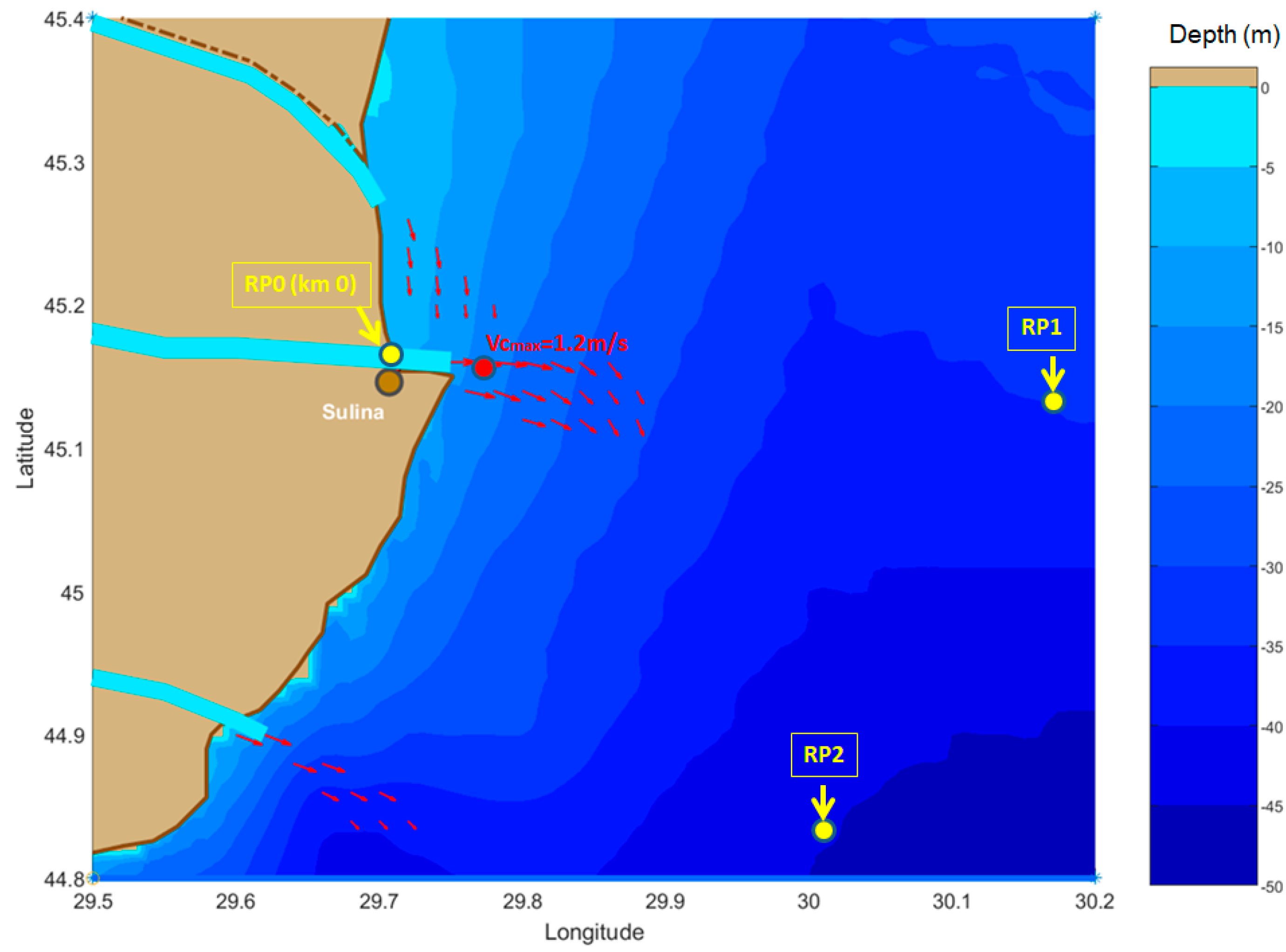
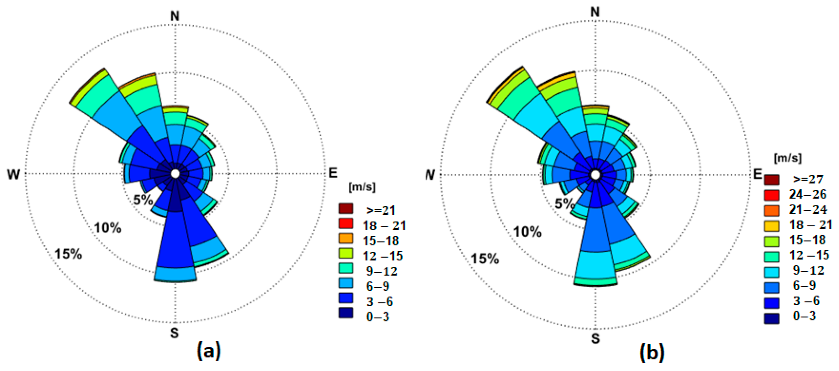
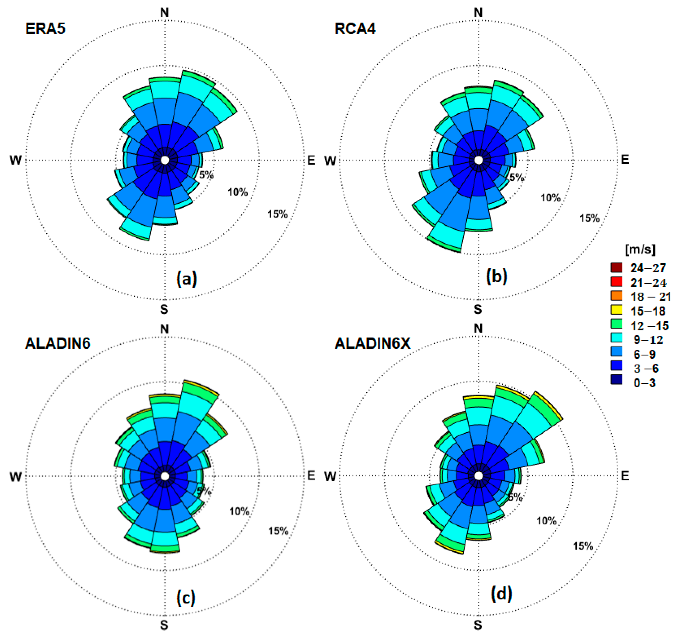
• The analysis of the wind data shows that there is in general a good match between the measurements and the model results, especially with regard to the intensity of the maximum wind speeds. However, by comparing Figure 4 and Figure 6, we can notice that in RP0, the dominant wind direction is from north to northwest, while in RP1, it is from north to northeast. Furthermore, unlike in RP0, in RP1, significant winds also come from the southeast, while in both cases, significant winds come from the south. The main explanation for these differences is that while RP1 is located 30 km offshore, RP0 represents the zero-kilometer point of the Danube, where both the influence of the coast and the local wind currents propagating along the river are more consistent.
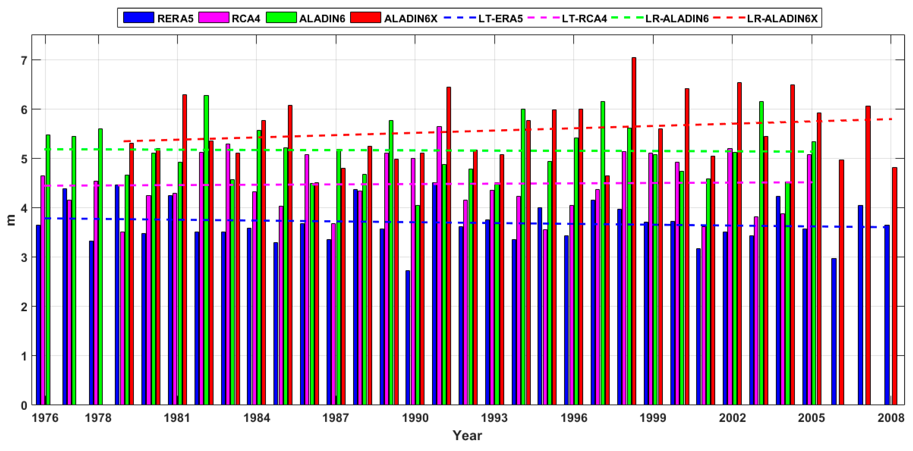
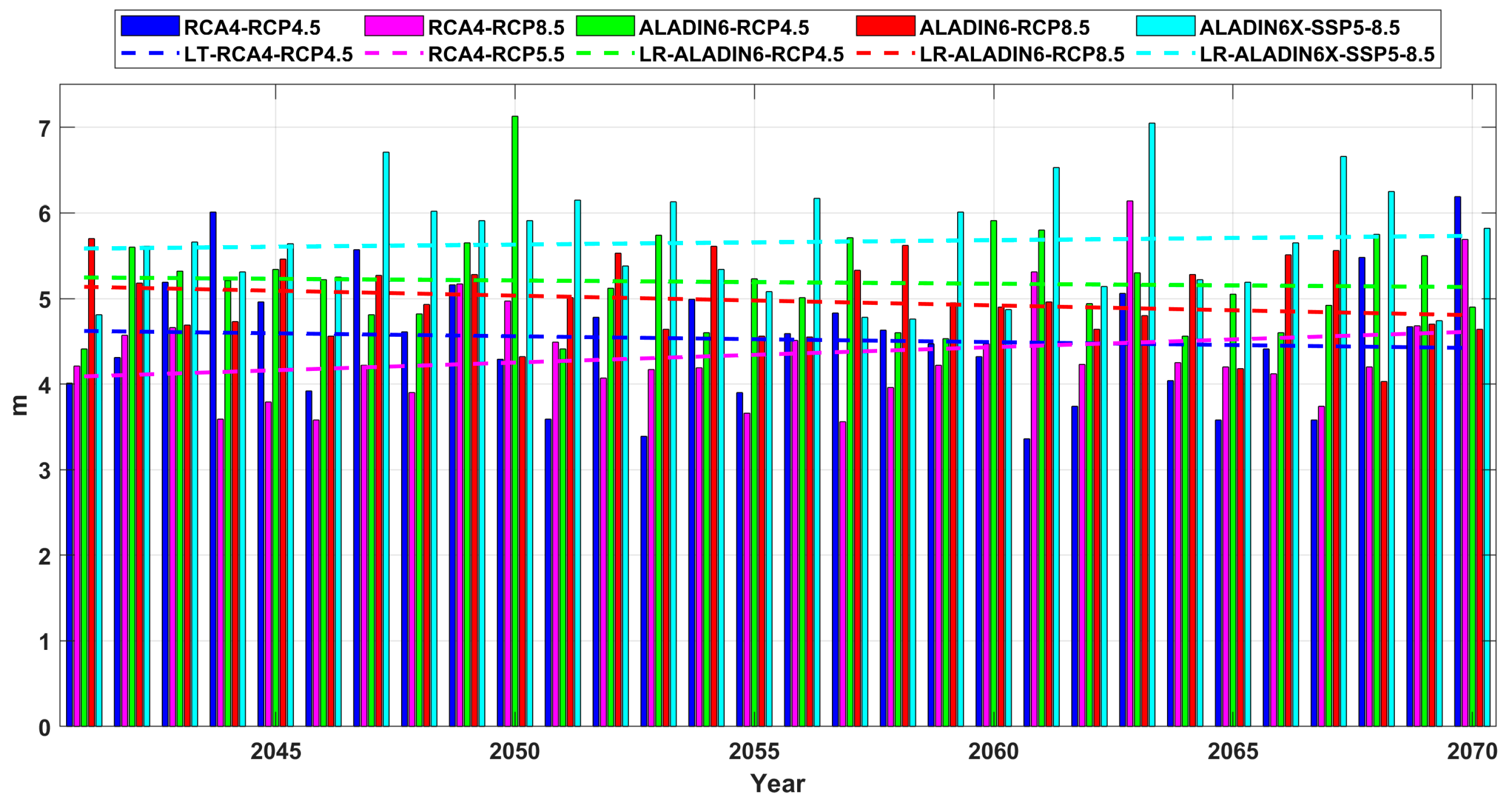
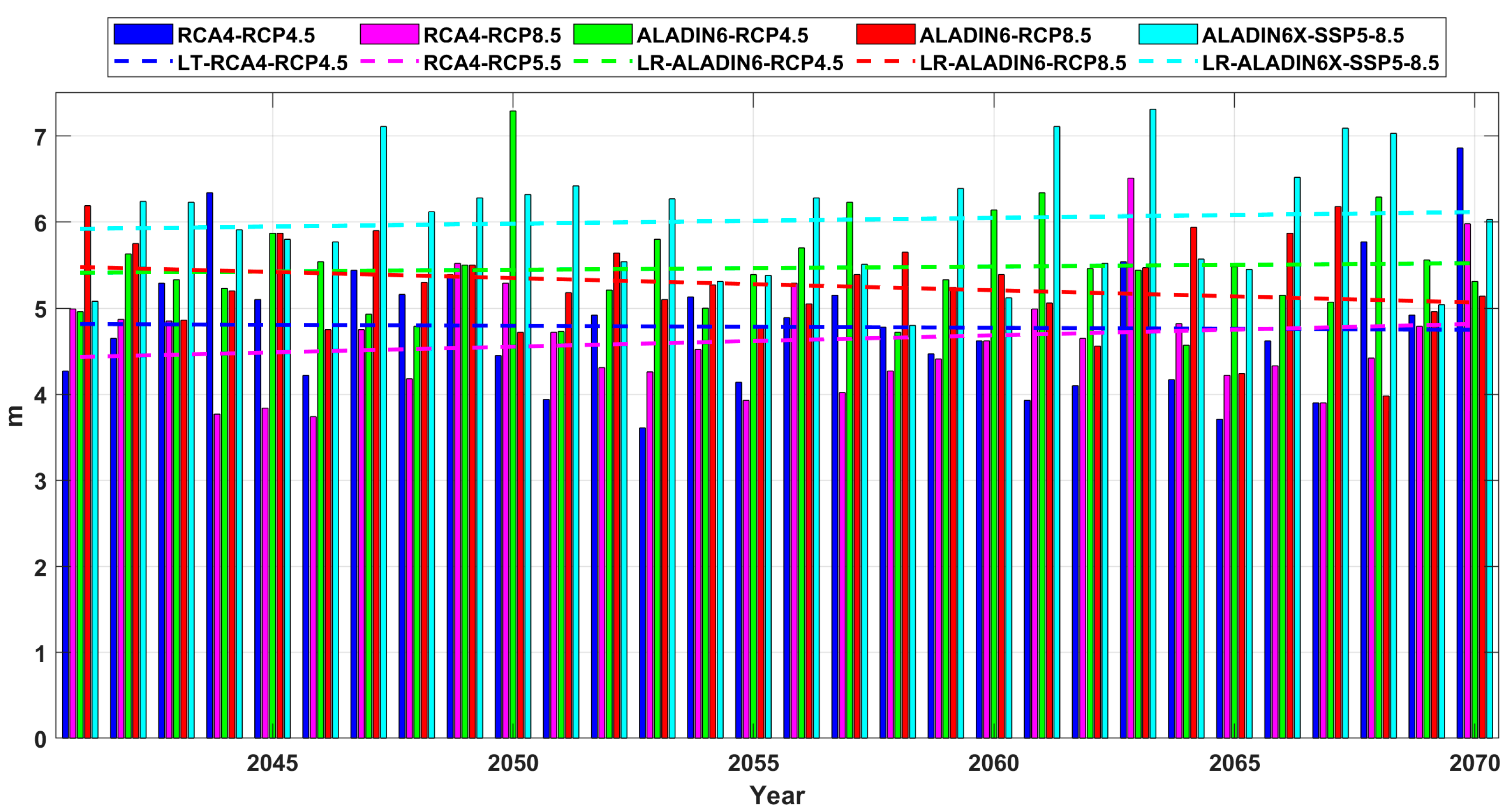
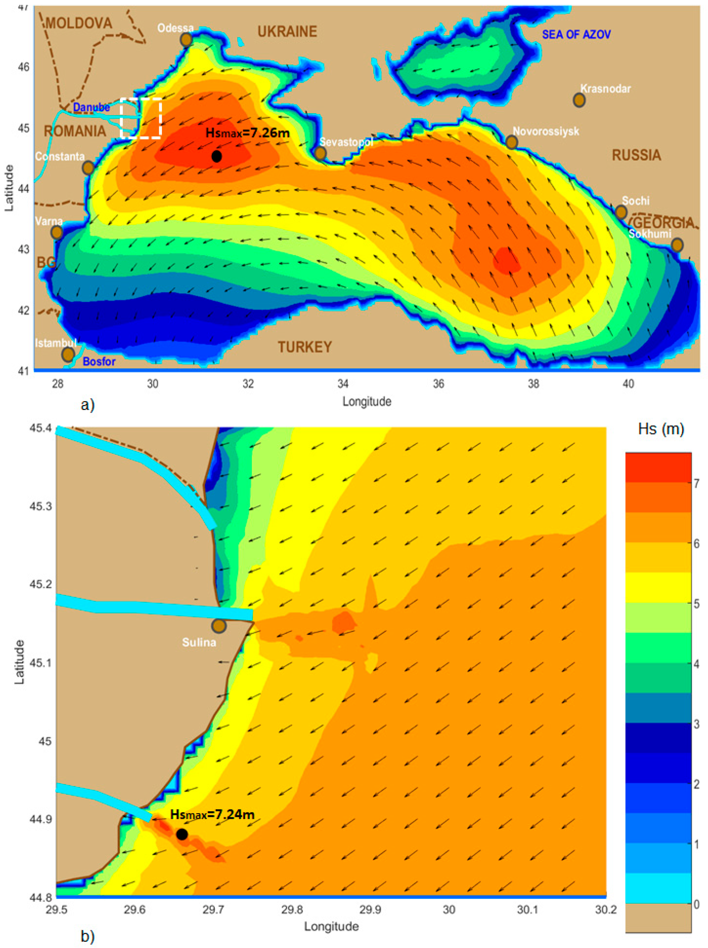
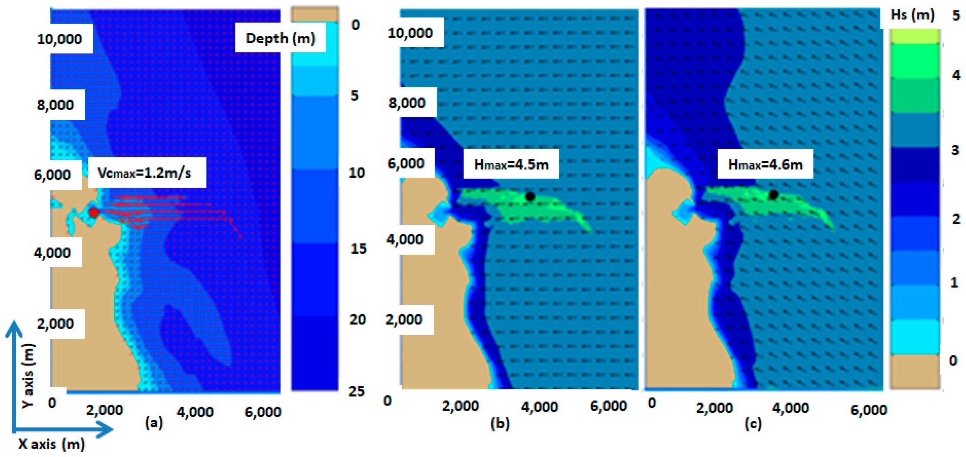
• With regard to the waves, the results show that we can expect significant wave heights that are even higher than 7 m in the coastal environment offshore the mouths of the Danube River. Furthermore, as Figure 14 clearly illustrates, the local processes and especially the wave–current interactions and the shallow water effects induce considerable enhancements in the wave height in the nearshore. From this perspective and in order to assess better the influence of the local effects at the entrance to the Sulina channel, wave model simulations were carried out considering the most common wave patterns from the point of view of the significant wave height (Hso) and the mean wave direction of the incoming waves on the offshore boundary (Wdir), as indicated by Figure 15, Figure 16, Figure 19 and Figure 20. Furthermore, previous results in terms of the wave modeling presented in reference [48] were also considered. Thus, in the high-resolution computational domain described in Table 1, SWAN simulations were performed considering significant wave heights and wave directions in the ranges of [1–5 m] and [30°–150°]. Based on the results of these simulations, an index giving the relative enhancement in the significant wave height at the entrance to the Sulina channel due to the wave–current interactions (RE_Hs) was evaluated. The expression of this index is given by the equation below, while the corresponding values are provided in

  Table 4. Results of the SWAN model simulations in the presence of currents considering various significant wave heights and mean wave directions incoming on the external boundary of the computational domain.

  Hso (m)	Wdir (°)
  	30		60		90		120		150
  	REHs (%)	BFI	REHs (%)	BFI	REHs (%)	BFI	REHs (%)	BFI	REHs (%)	BFI
  1	23	0.7	30	0.8	38	0.9	42	0.94	38	0.85
  2	17.5	1.2	25	1.5	36.5	1.75	38.5	1.4	27.5	1.3
  3	11	1.2	18.6	1.6	32.5	1.9	35	1.7	20.7	1.4
  4	8.25	1.1	15	1.5	30	1.8	31.75	1.6	17.75	1.4
  5	6	0.9	12.8	1.4	23.4	1.7	24.2	1.5	13.6	1.3

  .

$${RE}_{Hs}=\left({Hs}_{max}-Hso\right)/Hso$$

(10)

On the other hand, while spectral wave models such as SWAN are used to provide predictions in terms of the significant wave height, which represents four times the area under the spectral density, from the point of view of the navigation hazards, we are more interested in the prediction of the larger wave heights such as the maximum wave height. Usually, this is estimated based on some theoretical probabilistic distributions [49] among which the most common is the Rayleigh distribution [50], according to which waves with a maximum wave height of almost double the significant wave height can be often expected in a wave group. There are, however, situations when the ratio between the maximum and the significant wave height can be higher, or even much higher, than 2. Such kinds of waves are called freak or rogue waves, and they are very dangerous, inducing a high risk of hazards in navigation and many other marine activities. Thus, passing now from a statistical approach to a probabilistic one, we can estimate the higher risks of occurrences for such kinds of waves via the Benjamin–Feir index (BFI). The BFI, or the steepness-over-randomness ratio, was introduced by Jansen [51] and is defined as follows:

$$BFI=\sqrt{2\pi }St·Q_p$$

(11)

where St represents the integral wave steepness, representing the ratio between the significant wave height and the wavelength, and Q_p is the peakedness of the wave spectrum, defined as follows:

$$Q_p=2\frac{\iint \sigma E^2\left(\sigma ,\theta \right)d\sigma d\theta }{{\left(\iint \sigma E\left(\sigma ,\theta \right)d\sigma d\theta \right)}^2}$$

(12)

In fact, the BFI is a spectral shape parameter that can be related to the kurtosis of the wave height distribution, with the kurtosis depending on the square of the BFI. Experimental results indicate that for BFI = 0.2, the maximum wave heights are very well described by the Rayleigh distribution, while for BFI values greater than 0.9, the ratio of Hmax/Hs is substantially underestimated. The values of the BFI index corresponding to the most relevant wave propagation patterns are also presented in Table 4. The results indicate that BFI values higher than 1.5 occur in this area for waves with significant wave heights between 3 and 4 m and when the mean wave direction on the offshore boundary is between 90 and 120 degrees. From this perspective, two additional simulations were performed, considering the two situations presenting the highest risk from the point of view of the occurrence of rogue waves. The results are illustrated in Figure 23. Thus, Figure 23a presents the bathymetric map of the computational domain and the average current field. Figure 23b illustrates the results of the SWAN simulations in terms of the significant wave height scalar fields and wave vectors, considering offshore wave conditions of Hs = 3.5 m and a mean wave direction of 90 degrees. In Figure 23c, the same results are shown, considering offshore wave conditions of Hs = 3.5 m and a mean wave direction of 120 degrees. The values of the BFI index are indeed higher than those presented in Table 4, being 1.95 (with RE_Hs = 28.6%) for the simulations from Figure 23b and 1.9 (with RE_Hs = 31.4%) for that illustrated in Figure 23c. The above results indicate that, in addition to the enhancement in terms of Hs expressed by the values of the RE_Hs index, there is also a high risk of occurrence of abnormal waves for which the ratio between the maximum and the significant wave height is higher than 2.

5. Conclusions

The objective of this work was to study the past and future dynamics of the environmental matrix, especially wind and waves, at the entrance to the Sulina channel (the zero-kilometer point of the Danube). This represents the main southern entrance to the navigation system of Rhine–Main–Danube, the largest inland waterway in Europe linking the Black and the North Seas.

An analysis of 15 years of recent in situ measurements showed that the maximum value of the wind speed registered in this point was almost 31 m/s, while the maximum speed of the wind gust was almost 40 m/s, which was about 30% higher than the hourly value. The results also indicate that, for the entire data set analyzed, the average value of the ratio between the maximum speed of the wind gust and the hourly wind speed value was 1.7. However, in the case of the high wind speeds, the intensity of the wind gusts was relatively lower, and the values of the ratio between the maximum speed of the wind gusts and the hourly wind speed value was generally within the range of [1.3–1.4]. This means that wind gusts with speeds higher than 35 m/s are expected in this coastal area.

A second analysis was performed in two locations (one offshore Sulina and the other offshore Saint George) and was based on data provided by two regional wind climate models (RCA4 and ALADIN) under several scenarios (RCP4.5, RCP8.5, and SSP5-8.5). The analysis was performed for the future 30-year time interval (2041–2070). In order to compare the evolution of the wind climate in relation to the past conditions, a 30-year time interval from the past was also considered. For this period, the ERA5 reanalysis data were processed and analyzed in parallel with the RCM data. The climate model results indicated similar intensities for the past to those provided by the measurements for the maximum wind speed. All the models indicated maximum values of the wind speed that were higher than 25 m/s. It must also be highlighted that the time step considered for all the models was 3 h. The results show that slightly higher values are expected in the future for the wind speed compared to the past, especially in the case of SSP5-8.5.

The last analysis relates to the waves. In this connection, a wave modeling system that was previously validated against both in situ measurements and satellite data was forced successively with each wind data field considered. Simulations were performed for the two 30-year time periods that were previously defined in the case of the wind analysis. The results show that Hs values of about 7 m were encountered close to the mouths of the Danube in the past offshore. Such extreme values might be also expected more often in the future. The wave model simulations performed in the high-resolution computational domain that were focused on the Sulina channel also showed that, due to the nearshore effects, an enhancement between 30% and 40% in terms of wave height may be expected at the entrance to the Sulina channel. Furthermore, in addition to the significant wave heights being higher, due to the strong wave–current interaction processes, the probability of rogue waves occurring is very high. From this perspective, the results of the present work indicate that the most dangerous situations, from the point of view of a higher probability of the occurrence of rogue waves, correspond to the incoming waves with directions between 60° and 120° and significant wave heights higher than 2 m. This indicates that waves with heights of 20 m or greater and wind speeds higher than 30 m/s, associated with wind gusts that might exceed 40 m/s, can be expected in extreme storm conditions in this coastal environment.

Finally, based on the summarized three pillars of the above analysis, emphasizing the wind and wave extreme values that may occur as well as the conditions that can generate them, the general conclusion of this work is that the navigation conditions in this sector present a high risk of incidents and accidents, especially in the wintertime. In fact, for this reason, even in the case of moderate storms, the navigation is very often closed at the entrance to the Sulina channel. This work is still ongoing, and a next step would be to elaborate in more detail the risk assessment of severe shipping conditions, particularly focusing on the likelihood or probability of adverse conditions creating hazardous situations in this important navigation area.

References

1. United Nations. Report of the Conference of the Parties to the United Nations Framework Convention on Climate Change (21st Session); United Nations: Paris, France, 2015; Volume 4, p. 2017. [Google Scholar]
2. Moss, R.H.; Edmonds, J.A.; Hibbard, K.A.; Manning, M.R.; Rose, S.K.; Van Vuuren, D.P.; Carter, T.R.; Emori, S.; Kainuma, M.; Kram, T.; et al. The next generation of scenarios for climate change research and assessment. Nature 2010, 463, 747–756. [Google Scholar] [CrossRef] [PubMed]
3. Schleussner, C.-F. The Paris Agreement—The 1.5 °C Temperature Goal. Climate Analytics, January 2022. [Google Scholar]
4. IPCC. Managing the Risks of Extreme Events and Disasters to Advance Climate Change Adaptation; Field, C.B., Ed.; A Special Report of Working Groups I and II of the Intergovernmental Panel on Climate Change; Cambridge University Press: Cambridge, UK; New York, NY, USA, 2012; p. 582. [Google Scholar]
5. Toimil, A.; Losada, I.J.; Nicholls, R.J.; Dalrymple, R.A.; Stive, M.J.F. Addressing the challenges of climate change risks and adaptation in coastal areas: A review. Coast. Eng. 2020, 156, 103611. [Google Scholar] [CrossRef]
6. Rusu, E. A 30-year projection of the future wind energy resources in the coastal environment of the Black Sea. Renew. Energy 2019, 139, 228–234. [Google Scholar] [CrossRef]
7. Negm, A.; Zaharia, L.; Toroimac, G.I. The Lower Danube River Hydro-Environmental Issues and Sustainability; Springer: Berlin/Heidelberg, Germany, 2022; ISBN 978-3-031-03864-8. [Google Scholar]
8. Răileanu, A.B.; Rusu, L.; Rusu, E. An Evaluation of the Dynamics of Some Meteorological and Hydrological Processes along the Lower Danube. Sustainability 2023, 15, 6087. [Google Scholar] [CrossRef]
9. ShipTraffic.net, River Discharge and Related Historical Data from the European Flood Awareness System. Available online: http://www.shiptraffic.net/2001/04/danube-river-ship-traffic.html?full_screen=yes&map=vf (accessed on 12 February 2024).
10. Stagl, J.C.; Hattermann, F.F. Impacts of Climate Change on Riverine Ecosystems: Alterations of Ecologically Relevant Flow Dynamics in the Danube River and Its Major Tributaries. Water 2016, 8, 566. [Google Scholar] [CrossRef]
11. Maternová, A.; Materna, M.; Dávid, A. Revealing Causal Factors Influencing Sustainable and Safe Navigation in Central Europe. Sustainability 2022, 14, 2231. [Google Scholar] [CrossRef]
12. Galati Lower Danube River Administration, A.A. Available online: https://www.afdj.ro/en/content/ship-statistics (accessed on 12 February 2024).
13. Rouholahnejad Freund, E.; Abbaspour, K.C.; Lehmann, A. Water Resources of the Black Sea Catchment under Future Climate and Landuse Change Projections. Water 2017, 9, 598. [Google Scholar] [CrossRef]
14. Ivan, A.; Gasparotti, C.; Rusu, E. Influence of the interactions between waves and currents on the navigation at the entrance of the Danube delta. Protection and Sustainable Management of the Black Sea Ecosystem, Special Issue. J. Environ. Prot. Ecol. 2012, 13, 1673–1682. [Google Scholar]
15. Stanica, A.; Panin, N. Present evolution and future predictions for the deltaic coastal zone between the Sulina and Sf. Gheorghe Danube River mouths. Geomorphology 2009, 107, 41–46. [Google Scholar] [CrossRef]
16. Banescu, A.; Arseni, M.; Georgescu, L.P.; Rusu, E.; Iticescu, C. Evaluation of different simulation methods for analyzing flood scenarios in the Danube Delta. Appl. Sci. 2020, 10, 8327. [Google Scholar] [CrossRef]
17. Arseni, M.; Roșu, A.; Bocăneală, C.; Constantin, D.-E.; Georgescu, P.L. Flood hazard monitoring using GIS and remote sensing observations. Carpathian J. Earth Environ. Sci. 2017, 12, 329–334. [Google Scholar]
18. Onea, F.; Rusu, E. Wind energy assessments along the Black Sea basin. Meteorol. Appl. 2014, 21, 316–329. [Google Scholar] [CrossRef]
19. Bernardino, M.; Rusu, L.; Guedes Soares, C. Evaluation of extreme storm waves in the Black Sea. J. Oper. Oceanogr. 2021, 14, 114–128. [Google Scholar] [CrossRef]
20. Rusu, E. Modeling of wave-current interactions at the Danube’s mouths. J. Mar. Sci. Technol. 2010, 15, 143–159. [Google Scholar] [CrossRef]
21. Lazar, L.; Rodino, S.; Pop, R.; Tiller, R.; D’Haese, N.; Viaene, P.; De Kok, J.-L. Sustainable Development Scenarios in the Danube Delta—A Pilot Methodology for Decision Makers. Water 2022, 14, 3484. [Google Scholar] [CrossRef]
22. Novac, V.; Stavarache, G.; Rusu, E. Naval accidents causative factors—A Black Sea case study. Int. Multidiscip. Sci. GeoConference Surv. Geol. Min. Ecol. Manag. SGEM 2021, 21, 551–559. [Google Scholar]
23. Booij, N.; Ris, R.; Holthuijsen, L. A third generation wave model for coastal regions. Part 1: Model description and validation. J. Geophys. Res. 1999, 104, 7649–7666. [Google Scholar] [CrossRef]
24. ICPDR 2004, Danube Basin Analysis, WDF Report 2004. Available online: https://www.icpdr.org/sites/default/files/nodes/documents/danube_basin_analysis_2004.pdf (accessed on 2 December 2023).
25. Poncos, V.; Teleaga, D.; Bondar, C.; Oaie, G. A new insight on the water level dynamics of the Danube Delta using a high spatial density of SAR measurements. J. Hydrol. 2013, 482, 79–91. [Google Scholar] [CrossRef]
26. Bajo, M.; Ferrarin, C.; Dinu, I.; Umgiesser, G.; Stanica, A. The water circulation near the Danube Delta and the Romanian coast modelled with finite elements. Cont. Shelf Res. 2014, 78, 62–74. [Google Scholar] [CrossRef]
27. Romanian National Authority of Meteorology. 2024. Available online: https://www.meteoromania.ro/servicii/date-meteorologice/ (accessed on 14 September 2023).
28. ERA5/ECMWF. Available online: https://www.ecmwf.int/en/forecasts/datasets/reanalysis-datasets/era5 (accessed on 22 January 2024).
29. Giorgetta, M.A.; Jungclaus, J.; Reick, C.H.; Legutke, S.; Bader, J.; Böttinger, M.; Brovkin, V.; Crueger, T.; Esch, M.; Fieg, K.; et al. Climate and carbon cycle changes from 1850 to 2100 in MPI-ESM simulations for the Coupled Model Intercomparison Project phase 5. J. Adv. Model. Earth Syst. 2013, 5, 572–597. [Google Scholar] [CrossRef]
30. Giorgetta, M.; Jungclaus, J.; Reick, C.; Legutke, S.; Brovkin, V.; Crueger, T.; Esch, M.; Fieg, K.; Glushak, K.; Gayler, V.; et al. CMIP5 Simulations of the Max Planck Institute for Meteorology (MPI-M) Based on the MPI-ESM-LR Model: The piControl Experiment, Served by ESGF. World Data Center for Climate (WDCC) at DKRZ; PCMDI: San Francisco, CA, USA, 2012. [Google Scholar] [CrossRef]
31. COPERNICUS Database. Available online: https://cds.climate.copernicus.eu/cdsapp#!/dataset/projections-cordex-domains-single-levels?tab=form (accessed on 12 September 2023).
32. Nabat, P.; Somot, S.; Cassou, C.; Mallet, M.; Michou, M.; Bouniol, D.; Decharme, B.; Drugé, T.; Roehrig, R.; Saint-Martin, D. Modulation of radiative aerosols effects by atmospheric circulation over the Euro-Mediterranean region. Atmos. Chem. Phys. 2020, 20, 8315–8349. [Google Scholar] [CrossRef]
33. Roehrig, R.; Beau, I.; Saint-Martin, D.; Alias, A.; Decharme, B.; Guérémy, J.; Voldoire, A.; Abdel-Lathif, A.Y.; Bazile, E.; Belamari, S.; et al. The cnrm globalatmosphere model arpege-climat 6.3: Description and evaluation. J. Adv. Model. Earth Syst. 2020, 12, e2020MS002075. [Google Scholar] [CrossRef]
34. Darmaraki, S.; Somot, S.; Sevault, F.; Nabat, P. Past variability of Mediterranean Sea marine heatwaves. Geophys. Res. Lett. 2019, 46, 9813–9823. [Google Scholar] [CrossRef]
35. CNRM 2023. Available online: https://www.umr-cnrm.fr/spip.php?article1098&lang=fr (accessed on 14 March 2023).
36. Holthuijsen, H. Waves in Oceanic and Coastal Waters; Cambridge University Press: Cambridge, UK, 2007; p. 387. [Google Scholar]
37. Rusu, E. Strategies in using numerical wave models in ocean/coastal applications. J. Mar. Sci. Technol. 2011, 19, 58–75. [Google Scholar] [CrossRef]
38. WAMDI Group. The WAM model—A third generation ocean wave prediction model. J. Phys. Oceanogr. 1988, 18, 1775–1810. [CrossRef]
39. Tolman, H.L. A third-generation model for wind waves on slowly varying, unsteady and inhomogeneous depths and currents. J. Phys. Oceanogr. 1991, 21, 782–797. [Google Scholar] [CrossRef]
40. Rusu, L.; Bernardino, M.; Guedes Soares, C. Wind and wave modelling in the Black Sea. J. Oper. Oceanogr. 2014, 7, 520. [Google Scholar] [CrossRef]
41. Rusu, E. Reliability and Applications of the Numerical Wave Predictions in the Black Sea. Front. Mar. Sci. 2016, 3, 95. [Google Scholar] [CrossRef]
42. Rusu, E. Study of the Wave Energy Propagation Patterns in the Western Black Sea. Appl. Sci. 2018, 8, 993. [Google Scholar] [CrossRef]
43. Rusu, E. An analysis of the storm dynamics in the Black Sea. Ro. J. Techn. Sci. Appl. Mech. 2018, 63, 127–142. [Google Scholar]
44. Rusu, L. Assessment of the Wave Energy in the Black Sea Based on a 15-Year Hindcast with Data Assimilation. Energies 2015, 8, 1037010388. [Google Scholar] [CrossRef]
45. Rusu, L. A projection of the expected wave power in the Black Sea until the end of the 21st century. Renew. Energy 2020, 160, 136–147. [Google Scholar] [CrossRef]
46. Yan, X.; Su, X. Linear Regression Analysis: Theory and Computing; World Scientific: Singapore, 2009; pp. 1–2. ISBN 9789812834119. [Google Scholar]
47. Rusu, L.; Butunoiu, D.; Rusu, E. Analysis of the extreme storm events in the Black Sea considering the results of a ten-year wave hindcast. J. Environ. Prot. Ecol. 2014, 15, 445–454. [Google Scholar]
48. Rusu, E.; Soares, C.G. Modelling the effect of wave current interaction at the mouth of the Danube river. In Developments in Maritime Transportation and Exploitation of Sea Resources; CRC Press, Taylor & Francis Group: London, UK, 2013; pp. 979–986. [Google Scholar]
49. Nayaka, S.; Panchangb, V. A Note on Short-term Wave Height Statistics. Aquat. Procedia 2015, 4, 274–280. [Google Scholar] [CrossRef]
50. Longuuet-Higgins, M.S. On the Statistical Distribution of the Heights of Sea Waves. J. Mar. Res. 1952, 11, 245–265. [Google Scholar]
51. Janssen, P.A.E.M. Nonlinear four-wave interactions and freak waves. J. Phys. Oceanogr. 2003, 33, 863–883. [Google Scholar] [CrossRef]
Figure 1. The Black Sea and the main target area (the entrance to the Sulina channel). Figure processed from Google Earth.
Inventions 09 00041 g001
Figure 2. The bathymetric map of the coastal area at the Danube’s mouths and the position of the three reference points considered. The coastal currents induced by the river outflow, estimated according to references [24,25,26], are also represented with red arrows.
Inventions 09 00041 g002
Figure 3. Variations in the water level at the entrance to the Sulina channel (RP0). Results of the daily measurements carried out for the 15-year time interval of 2009–2023.
Inventions 09 00041 g003
Figure 4. Wind roses corresponding to the 15-year time interval of 2009–2023. (a) Uw—hourly averaged values of the wind speed; (b) Uwg—maximum value of the wind gust.
Inventions 09 00041 g004
Figure 5. Uw and Uwg represent annual maxim series measured at the entrance to the Sulina channel (RP0), corresponding to 15-year time interval of 2009–2023.
Inventions 09 00041 g005
Figure 6. Wind roses offshore the Sulina channel (RP1) for the recent past period based on an analysis of the hindcast and climate model data. (a) ERA5 (1976–2008); (b) RCA4 for the RCP scenarios (1976–2005); (c) ALADIN6 for the RCP scenarios (1976–2005); (d) ALADIN6x for the SSP scenario (1979–2008).
Inventions 09 00041 g006
Figure 7. Wind roses offshore the Saint George arm of the Danube (RP2) for the recent past period based on an analysis of the hindcast and climate model data. (a) ERA5 (1976–2008); (b) RCA4 for the RCP scenarios (1976–2005); (c) ALADIN6 for the RCP scenarios (1976–2005); (d) ALADIN6x for the SSP scenario (1979–2008).
Inventions 09 00041 g007
Figure 8. Wind speed (U10) annual maximum series and linear trends for the recent past period offshore Sulina (RP1). ERA5 (1976–2008), RCA4 and ALADIN6 (1976–2005), and ALADIN6x (1979–2008).
Inventions 09 00041 g008
Figure 9. Wind speed (U10) annual maximum series and linear trends for the recent past period offshore Saint George (RP2). ERA5 (1976–2008), RCA4 and ALADIN6 (1976–2005), and ALADIN6x (1979–2008).
Inventions 09 00041 g009
Figure 10. Wind roses offshore the Sulina channel (RP1) for the near future period (2041–2070) based on an analysis of the climate model data. (a) RCA4-RCP4.5; (b) RCA4-RCP8.5; (c) ALADIN6-RCP4.5; (d) ALADIN6-RCP8.5; (e) ALADIN6x-SSP5-8.5.
Inventions 09 00041 g010
Figure 11. Wind roses offshore Saint George (RP2) for the near future period (2041–2070) based on an analysis of the climate model data. (a) RCA4-RCP4.5; (b) RCA4-RCP8.5; (c) ALADIN6-RCP4.5; (d) ALADIN6-RCP8.5; (e) ALADIN6x-SSP5-8.5.
Inventions 09 00041 g011
Figure 12. Wind speed (U10) annual maximum series and linear trends, projections for the near future period (2041–2070) offshore Sulina (RP1). RCA4 (RCP4.5 and RCP8.5), ALADIN6 (RCP4.5 and RCP8.5), and ALADIN6x SSP5-8.5.
Inventions 09 00041 g012
Figure 13. Wind speed (U10) annual maximum series and linear trends, projections for the near future period (2041–2070) offshore Saint George (RP2). RCA4 (RCP4.5 and RCP8.5), ALADIN6 (RCP4.5 and RCP8.5), and ALADIN6x SSP5-8.5.
Inventions 09 00041 g013
Figure 14. Typical storm in the Black Sea: significant wave height scalar fields and wave vectors. SWAN model simulation corresponding to the timeframe 21.12.2004h03. (a) Black Sea basin; (b) coastal environment at the mouths of the Danube River.
Inventions 09 00041 g014
Figure 15. Hs wave roses offshore the Sulina channel (RP1) for the recent past period based on an analysis of the results provided by the wave modeling system forced with reanalysis and climate model data. The forcing wind fields considered are: (a) ERA5 (1976–2008); (b) RCA4 for the RCP scenarios (1976–2005); (c) ALADIN6 for the RCP scenarios (1976–2005); (d) ALADIN6x for the SSP scenario (1979–2008).
Inventions 09 00041 g015
Figure 16. Hs wave roses offshore the Saint George arm of the Danube (RP2) for the recent past period based on the analysis of the results provided by the wave modeling system forced with reanalysis and climate model data. The forcing wind fields considered are: (a) ERA5 (1976–2008); (b) RCA4 for the RCP scenarios (1976–2005); (c) ALADIN6 for the RCP scenarios (1976–2005); (d) ALADIN6x for the SSP scenario (1979–2008).
Inventions 09 00041 g016
Figure 17. Hs annual maximum series and linear trends for the recent past period offshore Sulina (RP1). Results of wave model simulations forced with the following wind fields: ERA5 (1976–2008), RCA4 and ALADIN6 (1976–2005), and ALADIN6x (1979–2008).
Inventions 09 00041 g017
Figure 18. Hs annual maximum series and linear trends for the recent past period offshore Saint George (RP2). Results of wave model simulations forced with the following wind fields: ERA5 (1976–2008), RCA4 and ALADIN6 (1976–2005), and ALADIN6x (1979–2008).
Inventions 09 00041 g018
Figure 19. Hs wave roses offshore the Sulina channel (RP1) for the near future period (2041–2070) based on the analysis of the results provided by the wave modeling system forced with the climate model data. The forcing wind fields considered are: (a) RCA4-RCP4.5; (b) RCA4-RCP8.5; (c) ALADIN6-RCP4.5; (d) ALADIN6-RCP8.5; (e) ALADIN6x-SSP5-8.5.
Inventions 09 00041 g019
Figure 20. Hs wave roses offshore the Saint George arm of the Danube (RP2) for the near future period (2041–2070) based on the analysis of the results provided by the wave modeling system forced with climate model data. The forcing wind fields considered are: (a) RCA4-RCP4.5; (b) RCA4-RCP8.5; (c) ALADIN6-RCP4.5; (d) ALADIN6-RCP8.5; (e) ALADIN6x-SSP5-8.5.
Inventions 09 00041 g020
Figure 21. Hs annual maximum series and linear trends, projections for the near future period (2041–2070) offshore Sulina (RP1). Results of wave model simulations forced with the following wind fields: RCA4 (RCP4.5 and RCP8.5), ALADIN6 (RCP4.5 and RCP8.5), and ALADIN6x SSP5-8.5.
Inventions 09 00041 g021
Figure 22. Hs annual maximum series and linear trends, projections for the near future period (2041–2070) offshore Saint George (RP2). Results of wave model simulations forced with the following wind fields: RCA4 (RCP4.5 and RCP8.5), ALADIN6 (RCP4.5 and RCP8.5), and ALADIN6x SSP5-8.5.
Inventions 09 00041 g022
Figure 23. Swan simulations in the high-resolution computational domain focused on the entrance to the Sulina channel. (a) Bathymetric map of the computational domain and current field (with red color); (b) significant wave height scalar fields and wave vectors considering the offshore wave conditions of Hs = 3.5 and a mean wave direction of 90 degrees; (c) significant wave height scalar fields and wave vectors considering offshore wave conditions of Hs = 3.5 m and a mean wave direction of 120 degrees.
Inventions 09 00041 g023