


Enhancing the Damage Detection and Classification of Unknown Classes with a Hybrid Supervised–Unsupervised Approach


 ,
, 
Abstract
1. Introduction
2. Methodology
2.1. Feature Extraction
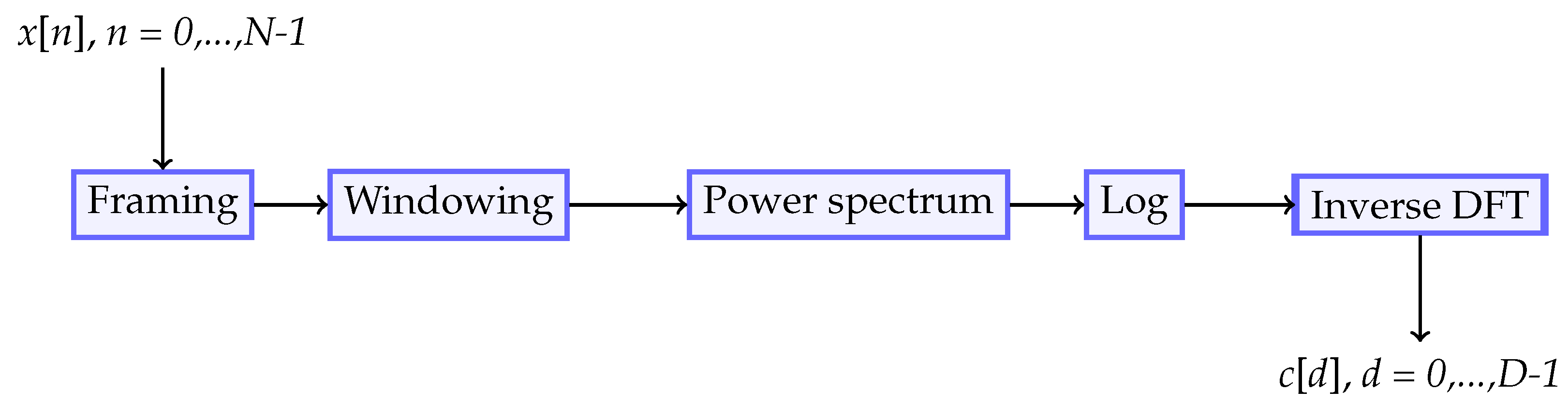
2.1.1. Cepstral Coefficients
2.1.2. Linear Discriminant Analysis
2.1.3. Probabilistic Linear Discriminant Analysis
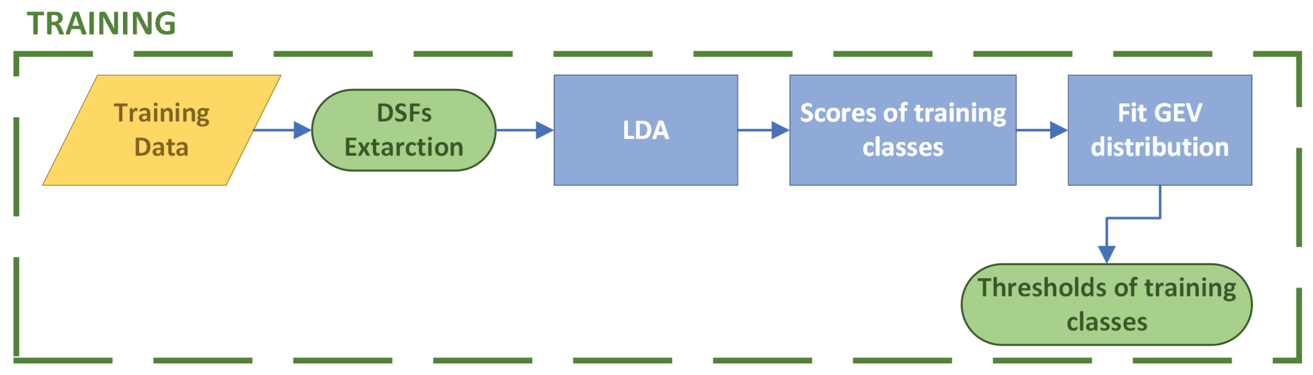
2.2. Training
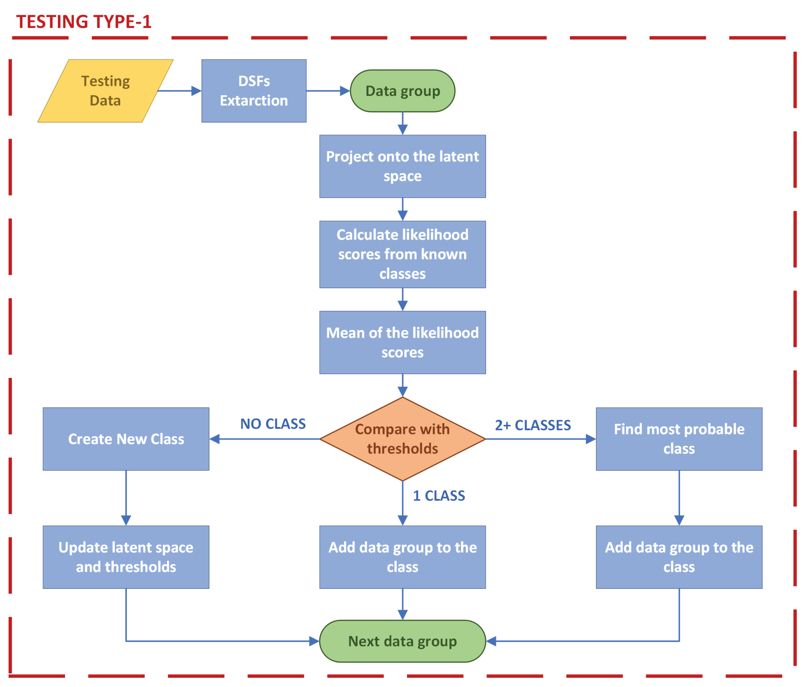
2.3. Testing Type 1
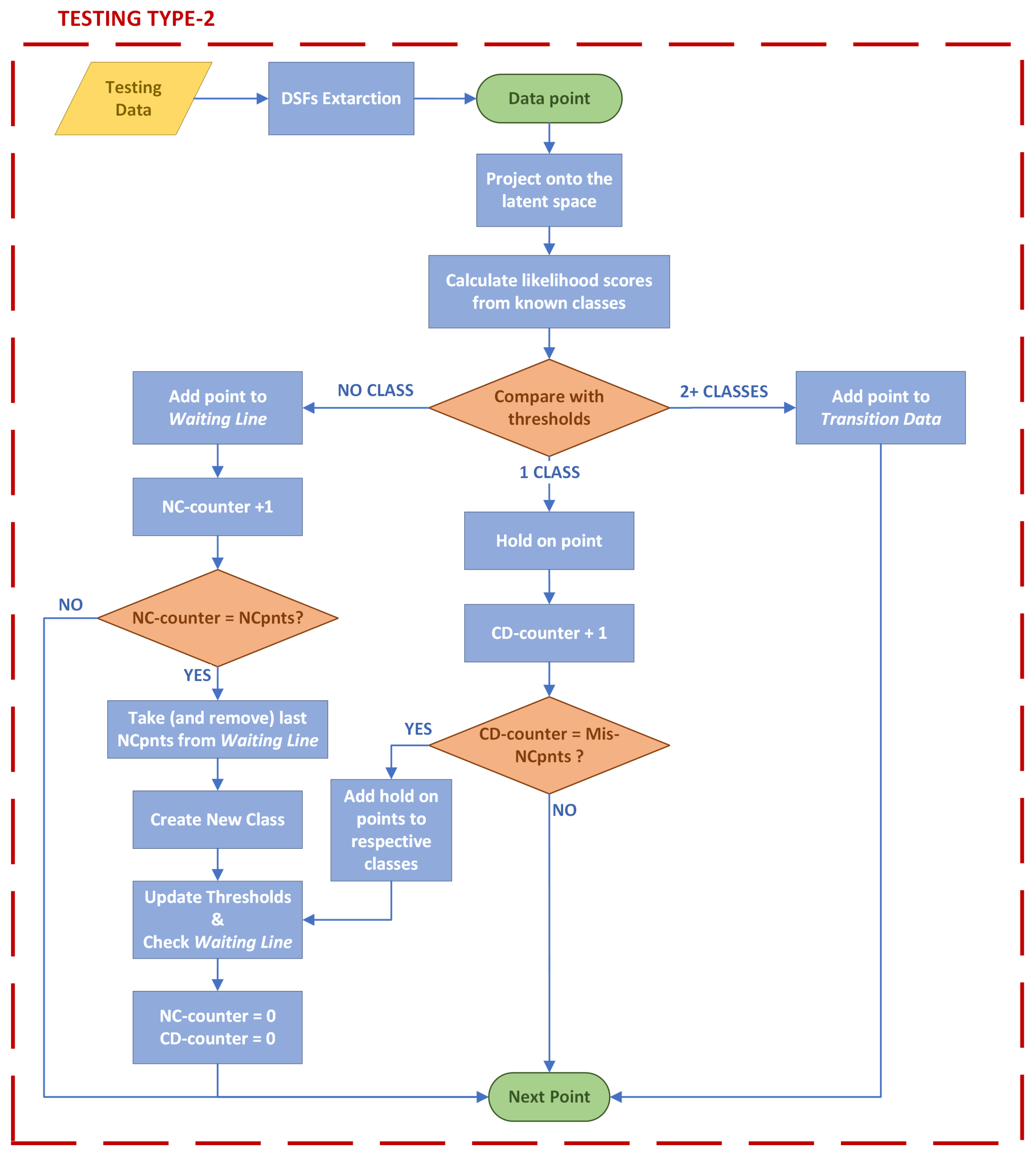
2.4. Testing Type 2
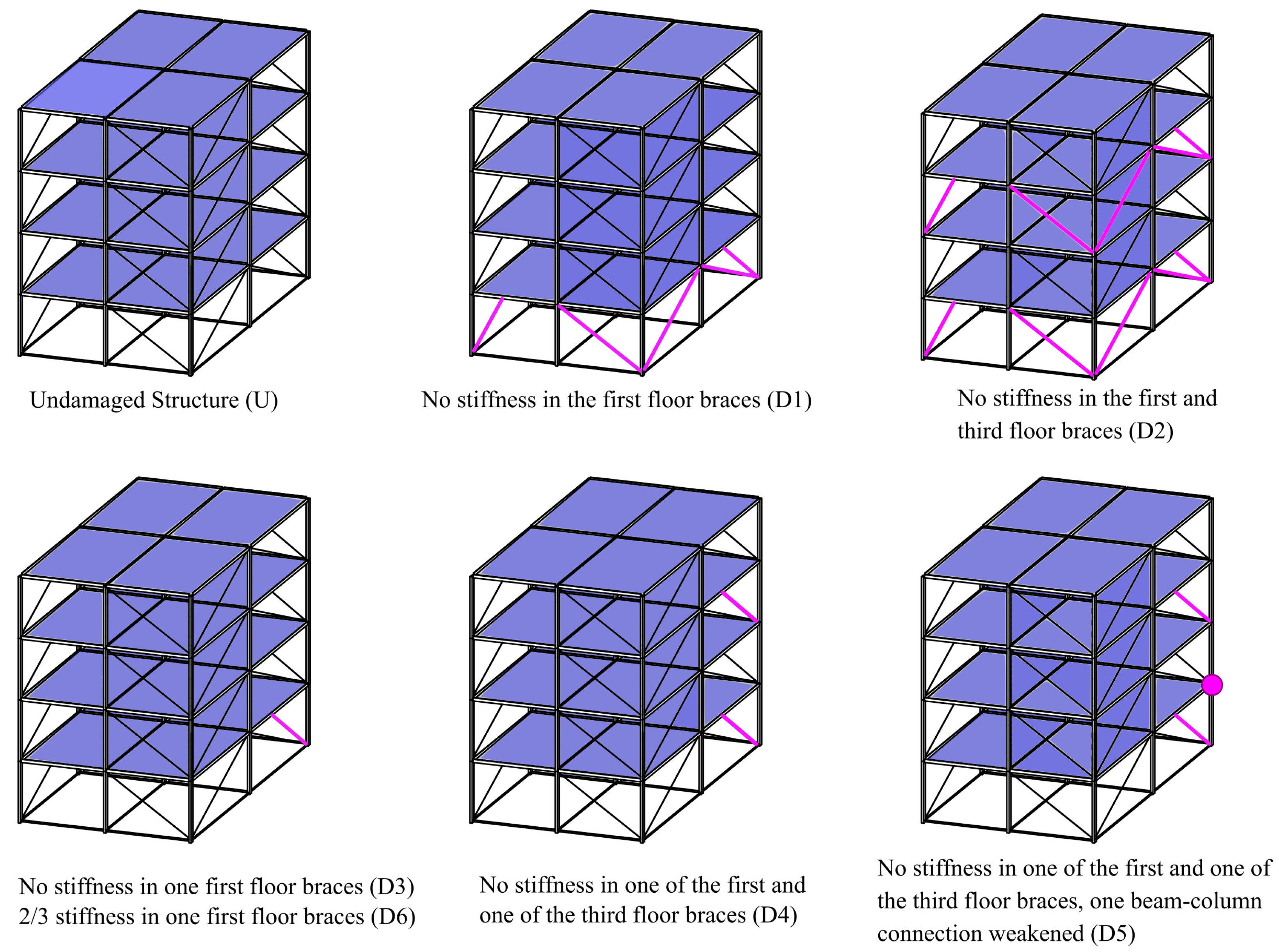
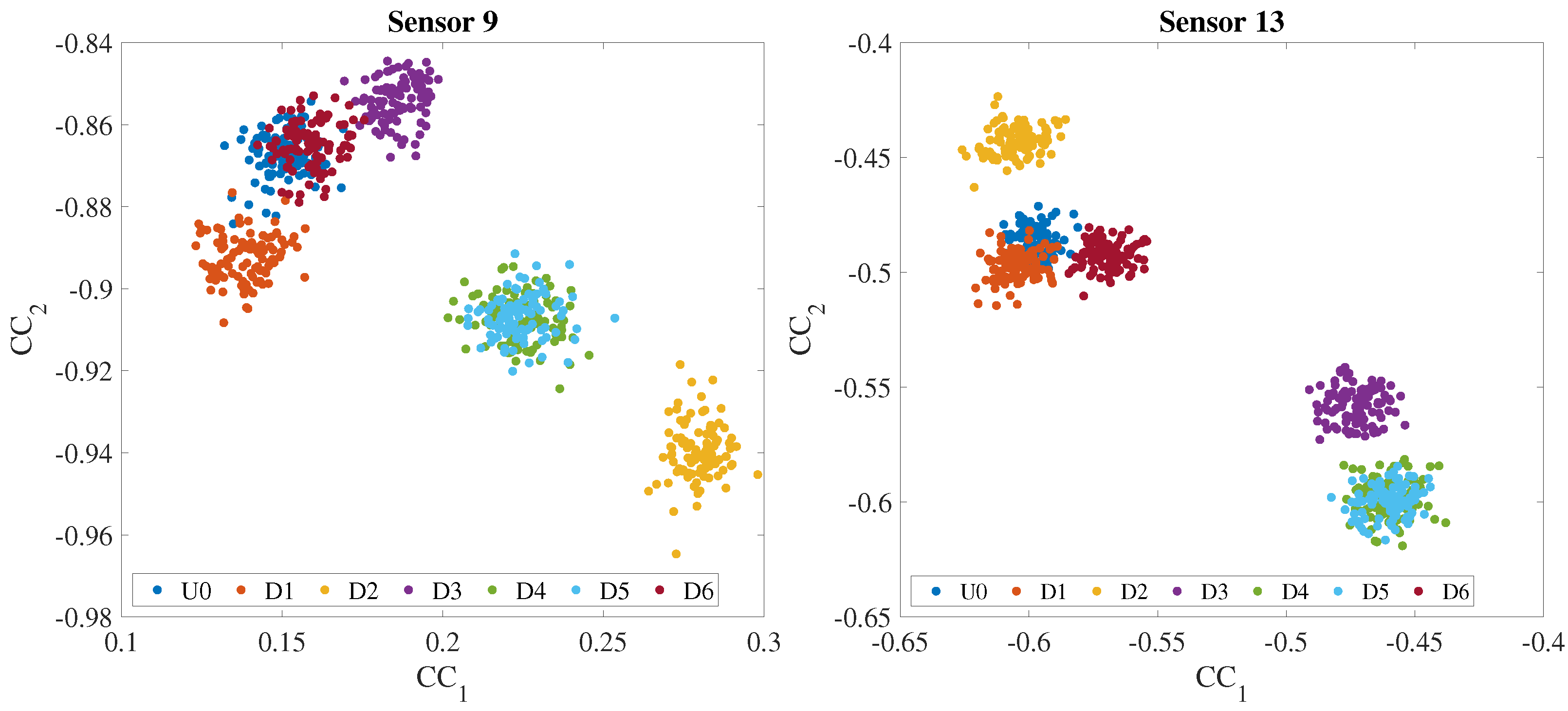
3. Case-Study 1: 12 DOF Numeric Dataset
3.1. Training Phase
3.2. Testing Type 1
3.3. Testing Type 2
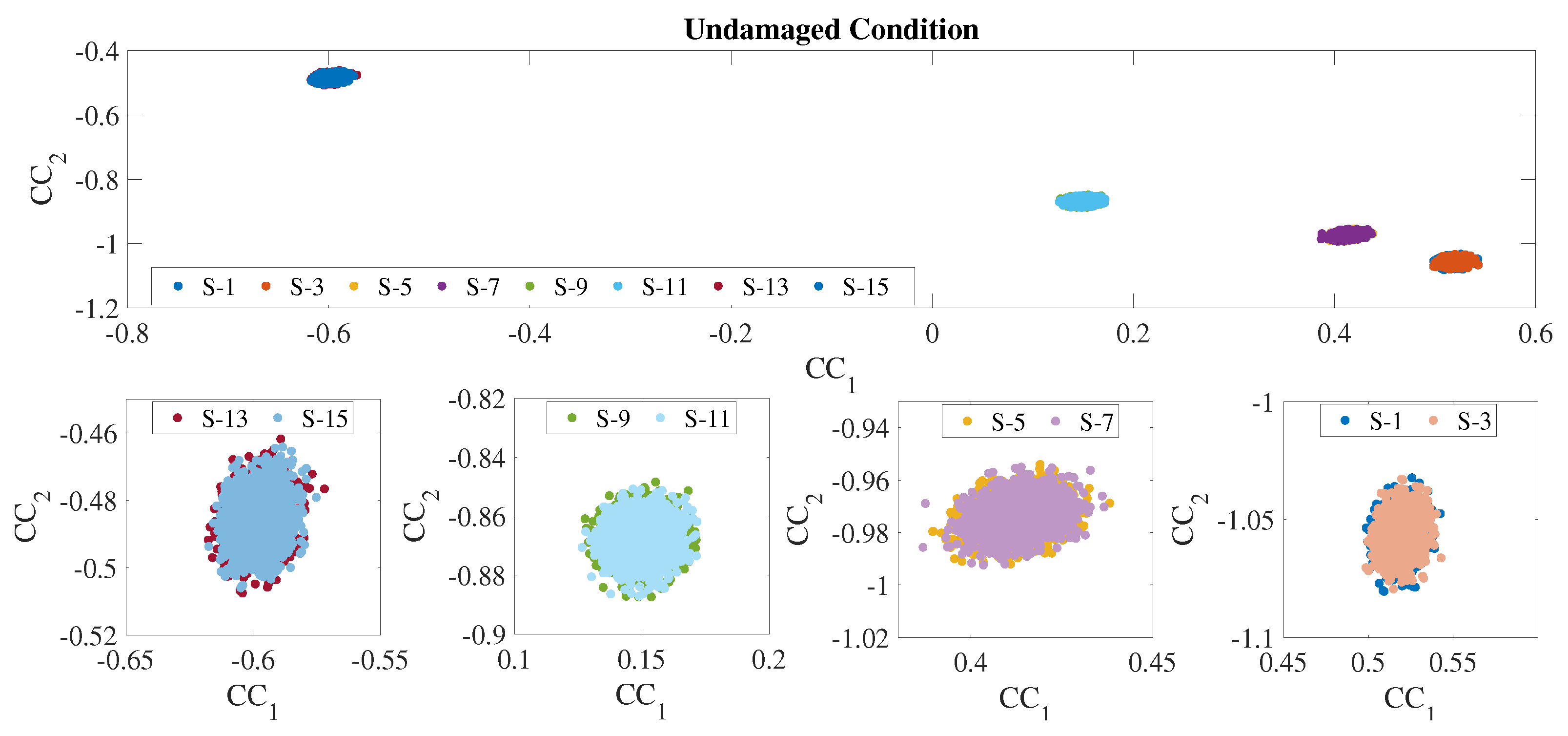
4. Case-Study 2: Z24 Bridge Experimental Data
4.1. The Z24 Bridge Dataset
4.2. Training Phase
4.3. Testing Type 1
4.4. Testing Type 2
5. Conclusions
Author Contributions
Funding
Data Availability Statement
Acknowledgments
Conflicts of Interest
References
- Farrar, C.R.; Worden, K. An introduction to structural health monitoring. Philos. Trans. R. Soc. A Math. Phys. Eng. Sci. 2007, 365, 303–315. [Google Scholar] [CrossRef]
- Gharehbaghi, V.R.; Noroozinejad Farsangi, E.; Noori, M.; Yang, T.; Li, S.; Nguyen, A.; Málaga-Chuquitaype, C.; Gardoni, P.; Mirjalili, S. A critical review on structural health monitoring: Definitions, methods, and perspectives. Arch. Comput. Methods Eng. 2021, 29, 2209–2235. [Google Scholar] [CrossRef]
- Fan, W.; Qiao, P. Vibration-based damage identification methods: A review and comparative study. Struct. Health Monit. 2011, 10, 83–111. [Google Scholar] [CrossRef]
- Hou, R.; Xia, Y. Review on the new development of vibration-based damage identification for civil engineering structures: 2010–2019. J. Sound Vib. 2021, 491, 115741. [Google Scholar] [CrossRef]
- Brownjohn, J.M.; Xia, P.Q.; Hao, H.; Xia, Y. Civil structure condition assessment by FE model updating: Methodology and case studies. Finite Elem. Anal. Des. 2001, 37, 761–775. [Google Scholar] [CrossRef]
- Friswell, M.; Mottershead, J.E. Finite Element Model Updating in Structural Dynamics; Springer Science & Business Media: Berlin, Germany, 1995; Volume 38. [Google Scholar]
- Cabboi, A.; Gentile, C.; Saisi, A. From continuous vibration monitoring to FEM-based damage assessment: Application on a stone-masonry tower. Constr. Build. Mater. 2017, 156, 252–265. [Google Scholar] [CrossRef]
- Ying, Y.; Garrett, J.H., Jr.; Oppenheim, I.J.; Soibelman, L.; Harley, J.B.; Shi, J.; Jin, Y. Toward data-driven structural health monitoring: Application of machine learning and signal processing to damage detection. J. Comput. Civ. Eng. 2013, 27, 667–680. [Google Scholar] [CrossRef]
- Tibaduiza Burgos, D.A.; Gomez Vargas, R.C.; Pedraza, C.; Agis, D.; Pozo, F. Damage identification in structural health monitoring: A brief review from its implementation to the use of data-driven applications. Sensors 2020, 20, 733. [Google Scholar] [CrossRef]
- Balafas, K.; Kiremidjian, A.S. Extraction of a series of novel damage sensitive features derived from the continuous wavelet transform of input and output acceleration measurements. Proc. Sens. Smart Struct. Technol. Civil Mech. Aerosp. Syst. 2014, 9061, 386–394. [Google Scholar]
- Worden, K.; Manson, G.; Fieller, N.R. Damage detection using outlier analysis. J. Sound Vib. 2000, 229, 647–667. [Google Scholar] [CrossRef]
- Farrar, C.R.; Worden, K. Structural Health Monitoring: A Machine Learning Perspective; John Wiley & Sons: Hoboken, NJ, USA, 2012. [Google Scholar]
- Cross, E.; Manson, G.; Worden, K.; Pierce, S. Features for damage detection with insensitivity to environmental and operational variations. Proc. R. Soc. A Math. Phys. Eng. Sci. 2012, 468, 4098–4122. [Google Scholar] [CrossRef]
- Gibbs, D.; Jankowski, K.; Rees, B.; Farrar, C.; Flynn, G. Identifying Environmental-and Operational-Insensitive Damage Features. In Data Science in Engineering, Volume 9: Proceedings of the 39th IMAC, A Conference and Exposition on Structural Dynamics 2021; Springer: Cham, Switzerland, 2022; pp. 105–121. [Google Scholar]
- Wang, Z.; Yang, D.H.; Yi, T.H.; Zhang, G.H.; Han, J.G. Eliminating environmental and operational effects on structural modal frequency: A comprehensive review. Struct. Control Health Monit. 2022, 29, e3073. [Google Scholar] [CrossRef]
- Tronci, E.M.; Betti, R.; De Angelis, M. Damage detection in a RC-masonry tower equipped with a non-conventional TMD using temperature-independent damage sensitive features. Dev. Built Environ. 2023, 15, 100170. [Google Scholar] [CrossRef]
- Kim, J.T.; Ryu, Y.S.; Cho, H.M.; Stubbs, N. Damage identification in beam-type structures: Frequency-based method vs mode-shape-based method. Eng. Struct. 2003, 25, 57–67. [Google Scholar] [CrossRef]
- Yao, R.; Pakzad, S.N. Autoregressive statistical pattern recognition algorithms for damage detection in civil structures. Mech. Syst. Signal Process. 2012, 31, 355–368. [Google Scholar] [CrossRef]
- Bernagozzi, G.; Achilli, A.; Betti, R.; Diotallevi, P.P.; Landi, L.; Quqa, S.; Tronci, E.M. On the use of multivariate autoregressive models for vibration-based damage detection and localization. Smart Struct. Syst. Int. J. 2021, 27, 335–350. [Google Scholar]
- Bogert, B.P. The quefrency alanysis of time series for echoes: Cepstrum, pseudoautocovariance, cross-cepstrum and saphe cracking. Proc. Symp. Time Ser. Anal. 1963, 209–243. [Google Scholar]
- Oppenheim, A.V.; Schafer, R.W. Discrete-Time Signal Processing; Prentice-Hall: Hoboken, NJ, USA, 1999; Volume 2, pp. 878–882. [Google Scholar]
- Davis, S.; Mermelstein, P. Comparison of parametric representations for monosyllabic word recognition in continuously spoken sentences. IEEE Trans. Acoust. Speech Signal Process. 1980, 28, 357–366. [Google Scholar] [CrossRef]
- Hasan, M.R.; Jamil, M.; Rahman, M. Speaker identification using mel frequency cepstral coefficients. Variations 2004, 1, 565–568. [Google Scholar]
- Nelwamondo, F.V.; Marwala, T.; Mahola, U. Early classifications of bearing faults using hidden Markov models, Gaussian mixture models, mel-frequency cepstral coefficients and fractals. Int. J. Innov. Comput. Inf. Control 2006, 2, 1281–1299. [Google Scholar]
- Benkedjouh, T.; Chettibi, T.; Saadouni, Y.; Afroun, M. Gearbox fault diagnosis based on mel-frequency cepstral coefficients and support vector machine. In Proceedings of the IFIP International Conference on Computational Intelligence and Its Applications, Oran, Algeria, 8–10 May 2018; pp. 220–231. [Google Scholar]
- Hwang, Y.R.; Jen, K.K.; Shen, Y.T. Application of cepstrum and neural network to bearing fault detection. J. Mech. Sci. Technol. 2009, 23, 2730–2737. [Google Scholar] [CrossRef]
- Balsamo, L.; Betti, R.; Beigi, H. A structural health monitoring strategy using cepstral features. J. Sound Vib. 2014, 333, 4526–4542. [Google Scholar] [CrossRef]
- de Souza, E.F.; Bittencourt, T.N.; Ribeiro, D.; Carvalho, H. Feasibility of Applying Mel-Frequency Cepstral Coefficients in a Drive-by Damage Detection Methodology for High-Speed Railway Bridges. Sustainability 2022, 14, 13290. [Google Scholar] [CrossRef]
- Tronci, E.M.; Beigi, H.; Betti, R.; Feng, M.Q. A damage assessment methodology for structural systems using transfer learning from the audio domain. Mech. Syst. Signal Process. 2023, 195, 110286. [Google Scholar] [CrossRef]
- Li, Z.; Lin, W.; Zhang, Y. Drive-by bridge damage detection using Mel-frequency cepstral coefficients and support vector machine. Struct. Health Monit. 2023, 22, 14759217221150932. [Google Scholar] [CrossRef]
- Morgantini, M.; Betti, R.; Balsamo, L. Structural damage assessment through features in quefrency domain. Mech. Syst. Signal Process. 2021, 147, 107017. [Google Scholar] [CrossRef]
- Li, L.; Morgantini, M.; Betti, R. Structural damage assessment through a new generalized autoencoder with features in the quefrency domain. Mech. Syst. Signal Process. 2023, 184, 109713. [Google Scholar] [CrossRef]
- Cunningham, P.; Cord, M.; Delany, S.J. Supervised learning. In Machine Learning Techniques for Multimedia: Case Studies on Organization and Retrieval; Springer: Berlin/Heidelberg, Germany, 2008; pp. 21–49. [Google Scholar]
- Perfetto, D.; Rezazadeh, N.; Aversano, A.; De Luca, A.; Lamanna, G. Composite Panel Damage Classification Based on Guided Waves and Machine Learning: An Experimental Approach. Appl. Sci. 2023, 13, 10017. [Google Scholar] [CrossRef]
- Moradi, M.; Broer, A.; Chiachío, J.; Benedictus, R.; Loutas, T.H.; Zarouchas, D. Intelligent health indicator construction for prognostics of composite structures utilizing a semi-supervised deep neural network and SHM data. Eng. Appl. Artif. Intell. 2023, 117, 105502. [Google Scholar] [CrossRef]
- Fugate, M.L.; Sohn, H.; Farrar, C.R. Unsupervised learning methods for vibration-based damage detection. In Proceedings of the 18th International Modal Analysis Conference–IMAC, San Antonio, TX, USA, 7–10 February 2000; Volume 18. [Google Scholar]
- Wang, Z.; Cha, Y.J. Unsupervised machine and deep learning methods for structural damage detection: A comparative study. Eng. Rep. 2022, e12551. [Google Scholar] [CrossRef]
- Roveri, N.; Carcaterra, A. Unsupervised identification of damage and load characteristics in time-varying systems. Contin. Mech. Thermodyn. 2015, 27, 531–550. [Google Scholar] [CrossRef]
- Rezazadeh, N.; de Oliveira, M.; Perfetto, D.; De Luca, A.; Caputo, F. Classification of Unbalanced and Bowed Rotors under Uncertainty Using Wavelet Time Scattering, LSTM, and SVM. Appl. Sci. 2023, 13, 6861. [Google Scholar] [CrossRef]
- Fogaça, M.J.; Cardoso, E.L.; de Medeiros, R. A systematic approach to find the hyperparameters of artificial neural networks applied to damage detection in composite materials. J. Braz. Soc. Mech. Sci. Eng. 2023, 45, 496. [Google Scholar] [CrossRef]
- Sarmadi, H.; Entezami, A. Application of supervised learning to validation of damage detection. Arch. Appl. Mech. 2021, 91, 393–410. [Google Scholar] [CrossRef]
- Xanthopoulos, P.; Pardalos, P.M.; Trafalis, T.B.; Xanthopoulos, P.; Pardalos, P.M.; Trafalis, T.B. Linear discriminant analysis. In Robust Data Mining; Springer: New York, NY, USA, 2013; pp. 27–33. [Google Scholar]
- Ioffe, S. Probabilistic linear discriminant analysis. In Proceedings of the Computer Vision–ECCV 2006: 9th European Conference on Computer Vision, Graz, Austria, 7–13 May 2006; Proceedings, Part IV 9. pp. 531–542. [Google Scholar]
- Snyder, D.; Garcia-Romero, D.; Sell, G.; Povey, D.; Khudanpur, S. X-vectors: Robust dnn embeddings for speaker recognition. In Proceedings of the 2018 IEEE International Conference on Acoustics, Speech and Signal Processing (ICASSP), Calgary, AB, Canada, 15–20 April 2018; pp. 5329–5333. [Google Scholar]
- Ananthram, A.; Saravanakumar, K.K.; Huynh, J.; Beigi, H. Multi-modal emotion detection with transfer learning. arXiv 2020, arXiv:2011.07065. [Google Scholar]
- Fisher, R.A. The use of multiple measurements in taxonomic problems. Ann. Eugen. 1936, 7, 179–188. [Google Scholar] [CrossRef]
- Rao, C.R. The utilization of multiple measurements in problems of biological classification. J. R. Stat. Soc. Ser. B 1948, 10, 159–203. [Google Scholar] [CrossRef]
- Kotz, S.; Nadarajah, S. Extreme Value Distributions: Theory and Applications; World Scientific: Singapore, 2000. [Google Scholar]
- Johnson, E.A.; Lam, H.F.; Katafygiotis, L.S.; Beck, J.L. Phase I IASC-ASCE structural health monitoring benchmark problem using simulated data. J. Eng. Mech. 2004, 130, 3–15. [Google Scholar] [CrossRef]
- Peeters, B.; De Roeck, G. One-year monitoring of the Z24-Bridge: Environmental effects versus damage events. Earthq. Eng. Struct. Dyn. 2001, 30, 149–171. [Google Scholar] [CrossRef]
- Roeck, G.D. The state-of-the-art of damage detection by vibration monitoring: The SIMCES experience. J. Struct. Control 2003, 10, 127–134. [Google Scholar] [CrossRef]
- Brincker, R.; Andersen, P.; Cantieni, R. Identification and level I damage detection of the Z24 highway bridge. Exp. Tech. 2001, 25, 51–57. [Google Scholar] [CrossRef]
- Krämer, C.; De Smet, C.; De Roeck, G. Z24 bridge damage detection tests. In IMAC 17, the International Modal Analysis Conference; Society of Photo-optical Instrumentation Engineers: Bellingham, WA, USA, 1999; Volume 3727, pp. 1023–1029. [Google Scholar]


| Scenario | Training | New or Existing Class | Predicted | Real | Correct? |
|---|---|---|---|---|---|
| Class | Class | ||||
| U0 | Seen | Existing Class | U0 | U0 | Yes |
| D1 | Unseen | New Class | D1 | D1 | Yes |
| D2 | Unseen | New Class | D2 | D2 | Yes |
| D3 | Unseen | New Class | D3 | D3 | Yes |
| D4 | Unseen | New Class | D4 | D4 | Yes |
| D5 | Unseen | Existing Class | D4 | D5 | No |
| D6 | Seen | Existing Class | D6 | D6 | Yes |
| Number | Date | Scenario |
|---|---|---|
| U01 | 04 August 1998 | Undamaged Condition |
| U02 | 09 August 1998 | Installation of pier settlement system |
| D01 | 10 August 1998 | Lowering of pier, 20 mm |
| D02 | 12 August 1998 | Lowering of pier, 40 mm |
| D03 | 17 August 1998 | Lowering of pier, 80 mm |
| D04 | 18 August 1998 | Lowering of pier, 95 mm |
| D05 | 19 August 1998 | Lifting of pier, tilt of foundation |
| D06 | 20 August 1998 | New reference condition |
| D07 | 26 August 1998 | Spalling of concrete at soffit, 12 m2 |
| D08 | 2 August 1998 | Spalling of concrete at soffit, 24 m2 |
| D09 | 27 August 1998 | Landslide of 1 m at abutment |
| D10 | 31 August 1998 | Failure of concrete hinge |
| D11 | 02 September 1998 | Failure of 2 anchor heads |
| D12 | 03 September 1998 | Failure of 4 anchor heads |
| D13 | 07 September 1998 | Rupture of 2 out of 16 tendons |
| D14 | 08 September 1998 | Rupture of 4 out of 16 tendons |
| D15 | 09 September 1998 | Rupture of 6 out of 16 tendons |
| Scenario | Training | New or Existing Class | Predicted | Real | Correct? |
|---|---|---|---|---|---|
| Class | Class | ||||
| U1 | Seen | Existing Class | 0 | 0 | Yes |
| D4 | Unseen | New Class | 1 | 1 | Yes |
| D6 | Seen | Existing Class | 2 | 2 | Yes |
| D8 | Unseen | New Class | 3 | 3 | Yes |
| D13 | Unseen | New Class | 4 | 4 | Yes |
| D14 | Unseen | Existing Class | 4 | 5 | Yes |
| Scenario | Training | New or Existing Class | Predicted | Real | Correct? |
|---|---|---|---|---|---|
| Class | Class | ||||
| U1 | Seen | Existing Class | 1 | 1 | Yes |
| U2 | Unseen | New Class | 2 | 2 | Yes |
| D1 | Unseen | New Class | 3 | 3 | Yes |
| D2 | Unseen | New Class | 4 | 4 | Yes |
| D3 | Unseen | New Class | 5 | 5 | Yes |
| D4 | Unseen | New Class | 6 | 6 | Yes |
| D5 | Unseen | New Class | 7 | 7 | Yes |
| D6 | Seen | Existing Class | 8 | 8 | Yes |
| D7 | Unseen | New Class | 9 | 9 | Yes |
| D8 | Unseen | Existing Class | 9 | 10 | No |
| D9 | Unseen | New Class | 11 | 11 | Yes |
| D10 | Unseen | New Class | 11 | 12 | No |
| D11 | Unseen | New Class | 13 | 13 | Yes |
| D12 | Unseen | Existing Class | 13 | 14 | No |
| D13 | Unseen | Existing Class | 13 | 15 | No |
| D14 | Unseen | Existing Class | 13 | 16 | No |
| D15 | Unseen | Existing Class | 13 | 17 | No |
Disclaimer/Publisher’s Note: The statements, opinions and data contained in all publications are solely those of the individual author(s) and contributor(s) and not of MDPI and/or the editor(s). MDPI and/or the editor(s) disclaim responsibility for any injury to people or property resulting from any ideas, methods, instructions or products referred to in the content. |
© 2024 by the authors. Licensee MDPI, Basel, Switzerland. This article is an open access article distributed under the terms and conditions of the Creative Commons Attribution (CC BY) license (https://creativecommons.org/licenses/by/4.0/).
Share and Cite
Stagi, L.; Sclafani, L.; Tronci, E.M.; Betti, R.; Milana, S.; Culla, A.; Roveri, N.; Carcaterra, A. Enhancing the Damage Detection and Classification of Unknown Classes with a Hybrid Supervised–Unsupervised Approach. Infrastructures 2024, 9, 40. https://doi.org/10.3390/infrastructures9030040
Stagi L, Sclafani L, Tronci EM, Betti R, Milana S, Culla A, Roveri N, Carcaterra A. Enhancing the Damage Detection and Classification of Unknown Classes with a Hybrid Supervised–Unsupervised Approach. Infrastructures. 2024; 9(3):40. https://doi.org/10.3390/infrastructures9030040
Chicago/Turabian StyleStagi, Lorenzo, Lorenzo Sclafani, Eleonora M. Tronci, Raimondo Betti, Silvia Milana, Antonio Culla, Nicola Roveri, and Antonio Carcaterra. 2024. "Enhancing the Damage Detection and Classification of Unknown Classes with a Hybrid Supervised–Unsupervised Approach" Infrastructures 9, no. 3: 40. https://doi.org/10.3390/infrastructures9030040
APA StyleStagi, L., Sclafani, L., Tronci, E. M., Betti, R., Milana, S., Culla, A., Roveri, N., & Carcaterra, A. (2024). Enhancing the Damage Detection and Classification of Unknown Classes with a Hybrid Supervised–Unsupervised Approach. Infrastructures, 9(3), 40. https://doi.org/10.3390/infrastructures9030040