
Bus Lane Design Based on Actual Traffic Loads and Climate Conditions


Abstract
:1. Introduction
2. Materials and Methods
2.1. Traffic
2.2. Climate Conditions
2.3. Material Properties
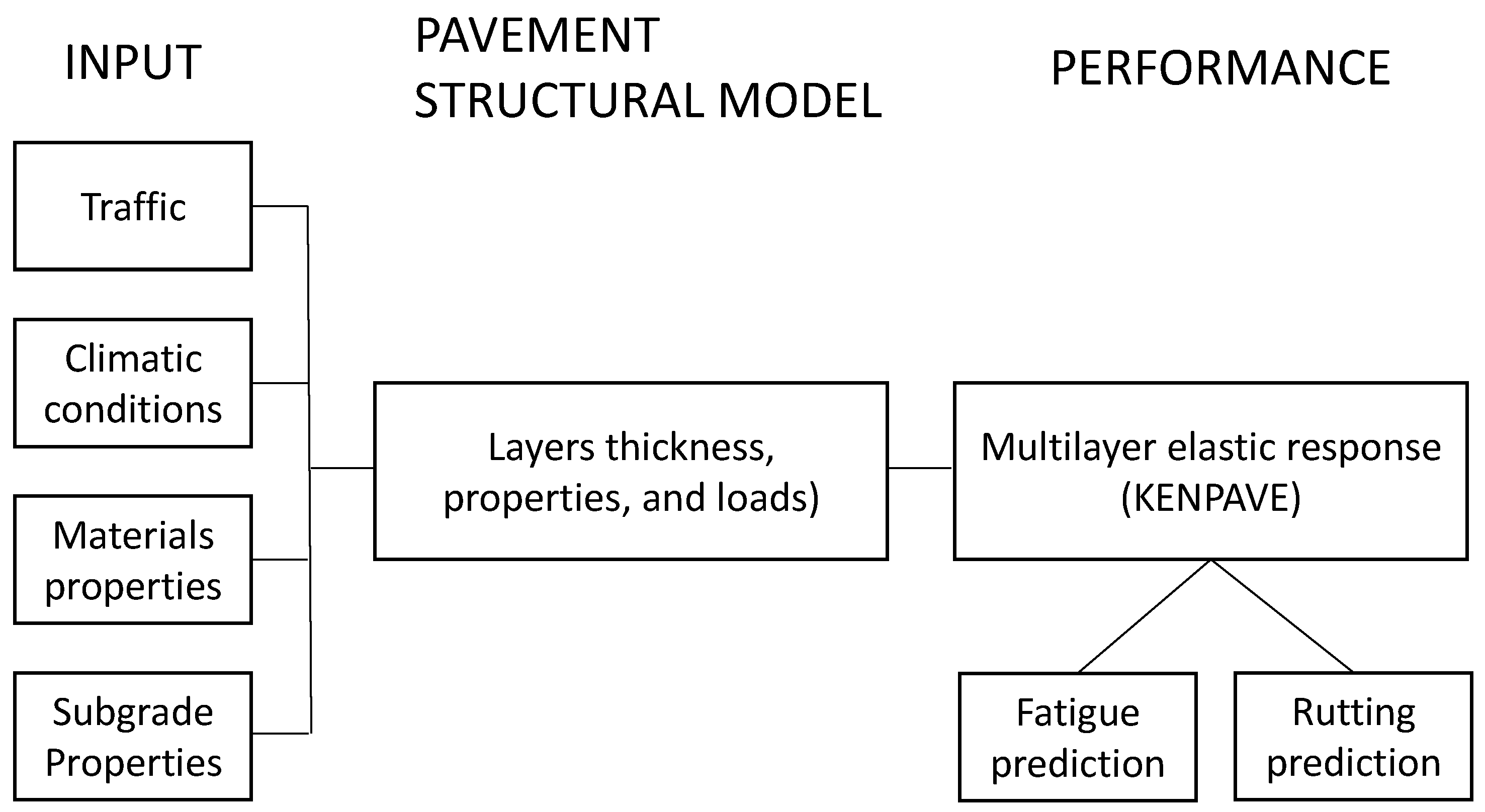
2.4. Pavement Structural Model
2.5. Fatigue Cracking
2.6. Rutting Law
3. Results
4. Conclusions
Author Contributions
Funding
Data Availability Statement
Acknowledgments
Conflicts of Interest
References
- Di Mascio, P.; De Rubeis, A.; De Marchis, C.; Germinario, A.; Metta, G.; Salzillo, R.; Moretti, L. Jointed Plain Concrete Pavements in Airports: Structural–Economic Evaluation and Proposal for a Catalogue. Infrastructures 2021, 6, 73. [Google Scholar] [CrossRef]
- Barber, S.D.; Knapton, J. Structural Design of Block Pavements for Ports. Concr. Block Paving 2011, 1, 141–149. [Google Scholar]
- Saudy, M.; Breakah, T.; El-Badawy, S.; Khedr, S. Development of a Flexible Pavement Design Catalogue Based on Mechanistic–Empirical Pavement Design Approach: Egyptian Case Study. Innov. Infrastruct. Solut. 2021, 6, 206. [Google Scholar] [CrossRef]
- Tavira, J.; Jiménez, J.R.; Ayuso, J.; López-Uceda, A.; Ledesma, E.F. Recycling Screening Waste and Recycled Mixed Aggregates from Construction and Demolition Waste in Paved Bike Lanes. J. Clean. Prod. 2018, 190, 211–220. [Google Scholar] [CrossRef]
- Barbudo, A.; Jiménez, J.R.; Ayuso, J.; Galvín, A.P.; Agrela, F. Catalogue of Pavements with Recycled Aggregates from Construction and Demolition Waste. Proceedings 2018, 2, 1282. [Google Scholar] [CrossRef]
- Colagrande, S.; Quaresima, R. Natural Cube Stone Road Pavements: Design Approach and Analysis. Transp. Res. Procedia 2023, 69, 37–44. [Google Scholar] [CrossRef]
- Di Mascio, P.; Moretti, L.; Capannolo, A. Concrete Block Pavements in Urban and Local Roads: Analysis of Stress-Strain Condition and Proposal for a Catalogue. J. Traffic Transp. Eng. Engl. Ed. 2019, 6, 557–566. [Google Scholar] [CrossRef]
- Richtlinien Für Die Standardisierung Des Oberbaus von Verkehrsflächen: RStO 12; Forschungsgesellschaft für Straßen- und Verkehrswesen, Ed.; FGSV; Forschungsges. für Strassen- und Verkehrswesen: Köln, Germany, 2012; ISBN 978-3-86446-021-0.
- Blab, R.; Eberhardsteiner, L. Neuer Oberbaukatalog Für Straßenaufbauten—RVS 03.08.63. Straße Autob. 2016, 67, 933–935. [Google Scholar]
- Corté, J.-F.; Goux, M.-T. Design of Pavement Structures: The French Technical Guide. Transp. Res. Rec. 1996, 1539, 116–124. [Google Scholar] [CrossRef]
- Vukobratović, N.; Barišić, I.; Josip Juraj Strossmayer University of Osijek, Faculty of Civil Engineering Osijek; Dimter, S. Analyses of the Influence of Material Characteristics on Pavement Design. Elektron. Časopis Građev. Fak. Osijek 2017, 8, 8–19. [Google Scholar] [CrossRef]
- Judycki, J.; Jaskuła, P.; Pszczoła, M.; Ryś, D.; Jaczewski, M.; Alenowicz, J.; Dołżycki, B.; Stienss, M. New Polish Catalogue of Typical Flexible and Semi-Rigid Pavements. MATEC Web. Conf. 2017, 122, 04002. [Google Scholar] [CrossRef]
- Hall, K. Long-Life Concrete Pavements in Europe and Canada; US Department of Transportation: Washington, DC, USA, 2007. [Google Scholar]
- Di Mascio, P.; Loprencipe, G.; Cantisani, G. Global Assessment Method of Road Distresses. Life-Cycle Struct. Syst. 2015, 4, 1113–1120. [Google Scholar] [CrossRef]
- Subagio, B.S.; Prayoga, A.B.; Fadilah, S.R. Implementation of Mechanistic-Empirical Pavement Design Guide against Indonesian Conditions Using Arizona Calibration. Open Civ. Eng. J. 2022, 16, e187414952210251. [Google Scholar] [CrossRef]
- Maina, J.W.; Denneman, E.; De Beer, M. Introduction of New Road Pavement Response Modelling Software by Means of Benchmarking. In Proceedings of the 27th Annual Southern African Transport Conference 2008, Pretoria, South Africa, 7–11 July 2008. [Google Scholar]
- Karadag, H.; Firat, S.; Isik, N.S.; Yilmaz, G. Determination of Permanent Deformation of Flexible Pavements Using Finite Element Model. Građevinar 2022, 74, 471–480. [Google Scholar]
- Awosanya, D.O.; Murana, A.A.; Olowosulu, A.T. Mechanistic—Empirical Flexible Pavement Analysis Using Load Spectra. FUOYE J. Eng. Technol. 2023, 8, 508–514. [Google Scholar] [CrossRef]
- CNR. Catalogo delle Pavimentazioni Stradali I, B.U. n. 178 Parte IV—Norme Tecniche. Consiglio Nazionale delle Ricerche: Roma, Italy, 1995. (In Italian)
- Marchionna, A.; Cesarini, M.; Fornaci, M.G.; Malgarini, M. Modello Di Degradazione Strutturale Delle Pavimentazioni. Autostrade 1985, 1, 85. [Google Scholar]
- Burmister, D. The General Theory of Stresses and Displacements in Layered Systems. I. J. Appl. Phys. 1945, 16, 89–94. [Google Scholar] [CrossRef]
- Mechanistic-Empirical Pavement Design Guide: A Manual of Practice; Interim ed.; American Association of State Highway and Transportation Officials: Washington, DC, USA, 2011; ISBN 978-1-56051-423-7.
- Behiry, A.E.A.E.-M. Fatigue and Rutting Lives in Flexible Pavement. Ain Shams Eng. J. 2012, 3, 367–374. [Google Scholar] [CrossRef]
- Brinchi, S.; Carrese, S.; Cipriani, E.; Colombaroni, C.; Crisalli, U.; Fusco, G.; Gemma, A.; Isaenko, N.; Mannini, L.; Petrelli, M. COVID-19 Transport Analytics: Analysis of Rome Mobility During Coronavirus Pandemic Era. In Proceedings of the Advances in Mobility-as-a-Service Systems; Nathanail, E.G., Adamos, G., Karakikes, I., Eds.; Springer International Publishing: Cham, Switzerland, 2021; pp. 1045–1055. [Google Scholar]
- S.T.A.T.U.S.|Roma Mobilità. Available online: https://romamobilita.it/it/progetti/studi-indagini/status (accessed on 28 June 2023).
- Adwan, I.; Milad, A.; Memon, Z.A.; Widyatmoko, I.; Ahmat Zanuri, N.; Memon, N.A.; Yusoff, N.I.M. Asphalt Pavement Temperature Prediction Models: A Review. Appl. Sci. 2021, 11, 3794. [Google Scholar] [CrossRef]
- Fiore, N.; Bruno, S.; Del Serrone, G.; Iacobini, F.; Giorgi, G.; Rinaldi, A.; Moretti, L.; Duranti, G.M.; Peluso, P.; Vita, L.; et al. Experimental Analysis of Hot-Mix Asphalt (HMA) Mixtures with Reclaimed Asphalt Pavement (RAP) in Railway Sub-Ballast. Materials 2023, 16, 1335. [Google Scholar] [CrossRef]
- Rasmussen, R.O.; Lytton, R.L.; Chang, G.K. Method to Predict Temperature Susceptibility of an Asphalt Binder. J. Mater. Civ. Eng. 2002, 14, 246–252. [Google Scholar] [CrossRef]
- Gunka, V.; Demchuk, Y.; Sidun, I.; Miroshnichenko, D.; Nyakuma, B.B.; Pyshyev, S. Application of Phenol-Cresol-Formaldehyde Resin as an Adhesion Promoter for Bitumen and Asphalt Concrete. Road Mater. Pavement Des. 2021, 22, 2906–2918. [Google Scholar] [CrossRef]
- Laurinavičius, A.; Ďygas, D. Thermal Conditions of Road Pavements and Their Influence on Motor Traffic. Transport 2003, 18, 23–31. [Google Scholar] [CrossRef]
- Consiglio Nazionale delle Ricerche. Catalogo delle Pavimentazioni Stradali. In Consiglio Nazionale delle Ricerche, Bollettino Ufficiale; Terra, M., Ed.; Consiglio Nazionale delle Ricerche: Rome, Italy, 1995; Volume 178, p. 95. (In Italian) [Google Scholar]
- Barber, E.S. Calculation of Maximum Pavement Temperatures from Weather Reports. Highw. Res. Board Bull. 1957, 168, 00237705. [Google Scholar]
- Witczak, M.W.; Fonseca, O.A. Revised Predictive Model for Dynamic (Complex) Modulus of Asphalt Mixtures. Transp. Res. Rec. 1996, 1540, 15–23. [Google Scholar] [CrossRef]
- Khattab, A.M.; El-Badawy, S.M.; Al Hazmi, A.A.; Elmwafi, M. Evaluation of Witczak E* Predictive Models for the Implementation of AASHTOWare-Pavement ME Design in the Kingdom of Saudi Arabia. Constr. Build. Mater. 2014, 64, 360–369. [Google Scholar] [CrossRef]
- Griffith, J.M.; Puzinauskas, V.P. Relation of Empirical Tests to Fundamental Viscosity of Asphalt Cement; ASTM International: West Conshohocken, PA, USA, 1963. [Google Scholar]
- Owais, M.; Moussa, G.S. Global Sensitivity Analysis for Studying Hot-Mix Asphalt Dynamic Modulus Parameters. Constr. Build. Mater. 2024, 413, 134775. [Google Scholar] [CrossRef]
- Fernando, E.G.; Liu, W. User’s Guide for the Modulus Temperature Correction Program (MTCP); Texas A&M Transportation Institute: College Station, TX, USA, 2000. [Google Scholar]
- Documenti Tecnici|Anas, S.p.A. Available online: https://www.stradeanas.it/it/lazienda/attivit%C3%A0/documenti-tecnici (accessed on 10 July 2023).
- Rada, G.; Witczak, M.W. Comprehensive Evaluation of Laboratory Resilient Moduli Results for Granular Material. Transp. Res. Rec. 1981, 810, 23–33. [Google Scholar]
- Huang, Y.H. Stresses and Strains in Viscoelastic Multilayer Systems Subjected to Moving Loads. Highw. Res. Rec. 1973, 457, 60–71. [Google Scholar]
- Zoccali, P.; Moretti, L.; Di Mascio, P.; Loprencipe, G.; D’Andrea, A.; Bonin, G.; Teltayev, B.; Caro, S. Analysis of Natural Stone Block Pavements in Urban Shared Areas. Case Stud. Constr. Mater. 2018, 8, 498–506. [Google Scholar] [CrossRef]
- Clauß, M.; Wellner, F. Influence of the Load Position of Heavy Vehicles on the Service Life of Asphalt Pavements. Int. J. Pavement Eng. 2023, 24, 2149962. [Google Scholar] [CrossRef]
- Chegenizadeh, A.; Keramatikerman, M.; Nikraz, H. Flexible Pavement Modelling Using Kenlayer. Electron. J. Geotech. Eng. 2016, 21, 2467–2479. [Google Scholar]
- Kiran, S.; Madhu, K. Rutting and Fatigue Analysis of Flexible Pavement Using KENPAVE and IITPAVE: A Review. J. Transp. Eng. Traffic Manag. 2022, 3, 1–12. [Google Scholar]
- Al Fatlawi, S.A.; Al-Jumaili, M.A. A Comparison of Viscoelastic Behaviour in Flexible Pavement Layers Responds to Different Contact Area. AIP Conf. Proc. 2024, 3009, 030105. [Google Scholar] [CrossRef]
- Wang, F.; Machemehl, R.B. Mechanistic–Empirical Study of Effects of Truck Tire Pressure on Pavement: Measured Tire–Pavement Contact Stress Data. Transp. Res. Rec. 2006, 1947, 136–145. [Google Scholar] [CrossRef]
- Taherkhani, H.; Moradloo, A.; Jalali Jirhandi, M. Investigation of the Effects of Tire Pressure on the Responses of Geosynthetic Reinforced Asphalt Pavement Using Finite Elements Methods. Q. J. Transp. Eng. 2016, 8, 323–342. [Google Scholar]
- Boulos Filho, P.; Raymundo, H.; Machado, S.T.; Leite, A.R.C.A.P.; Sacomano, J.B. Configurations of Tire Pressure on the Pavement for Commercial Vehicles: Calculation of the ‘N’Number and the Consequences on Pavement Performance. Indep. J. Manag. Prod. 2016, 7, 584–605. [Google Scholar] [CrossRef]
- Collop, A.C.; Cebon, D. A Theoretical Analysis of Fatigue Cracking in Flexible Pavements. Proc. Inst. Mech. Eng. Part C J. Mech. Eng. Sci. 1995, 209, 345–361. [Google Scholar] [CrossRef]
- Miner, M.A. Cumulative Damage in Fatigue. J. Appl. Mech. 1945, 12, A159–A164. [Google Scholar] [CrossRef]
- Sybilski, D.; Bańkowski, W. Asphalt Pavement Design Using Results of Laboratory Fatigue Tests of Asphalt Mixtures. Road Mater. Pavement Des. 2002, 3, 183–194. [Google Scholar] [CrossRef]
- Sudarsanan, N.; Kim, Y.R. A Critical Review of the Fatigue Life Prediction of Asphalt Mixtures and Pavements. J. Traffic Transp. Eng. Engl. Ed. 2022, 9, 808–835. [Google Scholar] [CrossRef]
- Pellinen, T.K.; Christensen, D.W.; Rowe, G.M.; Sharrock, M. Fatigue-Transfer Functions: How Do They Compare? Transp. Res. Rec. 2004, 1896, 77–87. [Google Scholar] [CrossRef]
- Sousa, J.B.; Ishai, I.; Svechinsky, G. Flexural Fatigue Tests and Predictions Models–Tools to Investigate SMA Mixes with New Innovative Binder Stabilizers. Four-Point Bend. 2012, 1, 171–188. [Google Scholar]
- Shafabakhsh, G.H.; Sadeghnejad, M.; Sajed, Y. Case Study of Rutting Performance of HMA Modified with Waste Rubber Powder. Case Stud. Constr. Mater. 2014, 1, 69–76. [Google Scholar] [CrossRef]
- Qiao, Y.; Flintsch, G.W.; Dawson, A.R.; Parry, T. Examining Effects of Climatic Factors on Flexible Pavement Performance and Service Life. Transp. Res. Rec. 2013, 2349, 100–107. [Google Scholar] [CrossRef]
- Bruno, S.; Del Serrone, G.; Di Mascio, P.; Loprencipe, G.; Ricci, E.; Moretti, L. Technical Proposal for Monitoring Thermal and Mechanical Stresses of a Runway Pavement. Sensors 2021, 21, 6797. [Google Scholar] [CrossRef]
- Fusco, R.; Moretti, L.; Fiore, N.; D’Andrea, A. Behavior Evaluation of Bituminous Mixtures Reinforced with Nano-Sized Additives: A Review. Sustainability 2020, 12, 8044. [Google Scholar] [CrossRef]
- Bell, H.P.; Howard, I.L.; Freeman, R.B.; Brown, E.R. Evaluation of Remaining Fatigue Life Model for Hot-Mix Asphalt Airfield Pavements. Int. J. Pavement Eng. 2012, 13, 281–296. [Google Scholar] [CrossRef]
- Ullidtz, P.; Harvey, J.; Tsai, B.-W.; Monismith, C. Calibration of CalME Models Using WesTrack Performance Data. In Research Report: UCPRC-RR-2006-14; University of California Pavement Research Center: Davis, CA, USA, 2006. [Google Scholar]


| Vehicles for Urban Mass Transport | Vehicles for Tourist Transport |
|---|---|
| Iveco Irisbus Citelis 12 m | Setra Comfort Class 12 m |
| Iveco Irisbus Citelis 18 m | Mercedes-Benz Turismo 12 m |
| Iveco Urban Way 12 m | Man Lion’s Coach 12 m |
| Mercedes-Benz Citaro 12 m | |
| Temsa Avenue 12 m |
| Vehicle Type | Illustration | Load Pattern | Axles Load ID and Weight (kN) |
|---|---|---|---|
| Bus 12 m |  |  | ↓A (75) ↓B (120) |
| Bus 18 m (articulated bus) |  |  | ↓A (75) ↓C (110) ↓B (120) |
| Vehicle Type | Illustration | Load Pattern | Axles Load ID and Weight (kN) |
|---|---|---|---|
| Old Bus 1 |  |  | ↓D (40) ↓E (80) |
| Old Bus 2 |  |  | ↓F (60) ↓G (100) |
| Time Slots | Seat Occupancy |
|---|---|
| 6:00 a.m.–8:59 a.m. | 100% |
| 9:00 a.m.–11:59 a.m. | 50% |
| 12:00 p.m.–2:59 p.m. | 70% |
| 3:00 p.m.–5:59 p.m. | 50% |
| 6:00 p.m.–8:59 p.m. | 100% |
| 09:00 p.m.–5:59 a.m. | 30% |
| Bus Length | Axle ID | Maximum Weight (kN) | Curb Weight (kN) | Gross Vehicle Weight (kN) |
|---|---|---|---|---|
| 12 m | A | 75 | 44 | 31 |
| B | 120 | 76 | 44 | |
| 18 m | A | 75 | 42 | 33 |
| C | 110 | 66 | 44 | |
| B | 120 | 72 | 48 |
| Season | Month | Number of Passages | |||
|---|---|---|---|---|---|
| BL1 | BL2 | BL3 | BL4 | ||
| Winter | January | 18,684 | 18,643 | 10,066 | 10,704 |
| February | 17,015 | 17,121 | 10,168 | 10,888 | |
| March | 19,360 | 19,380 | 10,738 | 11,212 | |
| Spring | April | 18,339 | 18,228 | 10,194 | 10,482 |
| May | 13,143 | 13,822 | 10,454 | 10,054 | |
| June | 12,544 | 11,345 | 10,322 | 9436 | |
| Summer | July | 11,252 | 10,244 | 9655 | 8710 |
| August | 10,875 | 10,945 | 9435 | 8546 | |
| September | 17,126 | 17,422 | 10,788 | 9947 | |
| Autumn | October | 19,835 | 19,856 | 11,064 | 10,727 |
| November | 19,211 | 17,843 | 11,546 | 14,568 | |
| December | 19,586 | 18,517 | 11,455 | 12,075 | |
| Total | 196,970 | 193,366 | 125,885 | 127,349 | |
| Season | Month | Vehicles Passages | |||
|---|---|---|---|---|---|
| BL1 | BL2 | BL3 | BL4 | ||
| Winter | January | 391,974 | 391,114 | 224,560 | 212,232 |
| February | 356,960 | 359,183 | 213,316 | 214,382 | |
| March | 406,156 | 406,575 | 225,274 | 226,400 | |
| Spring | April | 384,736 | 382,407 | 213,861 | 214,930 |
| May | 275,729 | 289,973 | 219,316 | 220,412 | |
| June | 263,162 | 238,008 | 216,546 | 217,629 | |
| Summer | July | 236,057 | 214,910 | 202,553 | 203,566 |
| August | 228,148 | 229,616 | 197,938 | 198,928 | |
| September | 359,288 | 365,498 | 226,323 | 227,454 | |
| Autumn | October | 416,121 | 416,561 | 232,113 | 233,273 |
| November | 403,030 | 374,330 | 242,225 | 243,436 | |
| December | 410,897 | 388470 | 240,316 | 241,517 | |
| 4,132,256 | 4,056,648 | 2,654,341 | 2654161 | ||
| Season | Seasonal Average Air Temperature (T) | Seasonal Average Air Temperature Variation (TV) | Seasonal Average Solar Irradiance (SI) | Annual Average Wind Speed (w) |
|---|---|---|---|---|
| [°C] | [°C] | [kcal/m2] | [km/h] | |
| Winter | 4.5 | 6.0 | 2718 | 13.00 |
| Spring | 11.5 | 7.5 | 5785 | |
| Summer | 22.0 | 10.6 | 6507 | |
| Autumn | 14.0 | 9.3 | 3547 |
| Coefficient | AC-20 (Wearing Course) | AC-10 (Binder Course) | AC-2.5 (Base Course) |
|---|---|---|---|
| A | 10.9168 | 11.0770 | 11.8408 |
| VTS | −3.6469 | −3.7097 | −3.9974 |
| Layer | Winter Moduli (MPa) | |||||
|---|---|---|---|---|---|---|
| 6:00 a.m.–8:59 a.m. | 9:00 a.m.–11:59 a.m. | 12:00 p.m.–2:59 p.m. | 3:00 p.m.–5:59 p.m. | 6:00 p.m.–8:59 p.m. | 9:00 p.m.–5:59 a.m. | |
| Wearing | 13,373 | 11,125 | 10,351 | 11,370 | 13,750 | 16,368 |
| Binder | 16,419 | 14,149 | 12,781 | 12,974 | 14,642 | 17,894 |
| Base | 16,733 | 15,696 | 14,512 | 13,864 | 14,093 | 16,108 |
| Layer | Spring Moduli (MPa) | |||||
|---|---|---|---|---|---|---|
| 6:00 a.m.–8:59 a.m. | 9:00 a.m.–11:59 a.m. | 12:00 p.m.–2:59 p.m. | 3:00 p.m.–5:59 p.m. | 6:00 p.m.–8:59 p.m. | 9:00 p.m.–5:59 a.m. | |
| Wearing | 7081 | 4466 | 3741 | 4714 | 7594 | 11722 |
| Binder | 9125 | 6316 | 4926 | 5108 | 6873 | 11279 |
| Base | 9323 | 7955 | 6552 | 5854 | 6095 | 8483 |
| Layer | Summer Moduli (MPa) | |||||
|---|---|---|---|---|---|---|
| 6:00 a.m.–8:59 a.m. | 9:00 a.m.–11:59 a.m. | 12:00 p.m.–2:59 p.m. | 3:00 p.m.–5:59 p.m. | 6:00 p.m.–8:59 p.m. | 9:00 p.m.–5:59 a.m. | |
| Wearing | 4909 | 3005 | 2500 | 3180 | 5299 | 8623 |
| Binder | 6249 | 4205 | 3240 | 3365 | 4601 | 7903 |
| Base | 6288 | 5290 | 4296 | 3815 | 3980 | 5671 |
| Layer | Autumn Moduli (MPa) | |||||
|---|---|---|---|---|---|---|
| 6:00 a.m.–8:59 a.m. | 9:00 a.m.–11:59 a.m. | 12:00 p.m.–2:59 p.m. | 3:00 p.m.–5:59 p.m. | 6:00 p.m.–8:59 p.m. | 9:00 p.m.–5:59 a.m. | |
| Wearing | 11,344 | 9515 | 8891 | 9713 | 11,654 | 13,843 |
| Binder | 13,675 | 11,850 | 10,761 | 10,914 | 12,244 | 14,878 |
| Base | 13,789 | 12,955 | 12,012 | 11,498 | 11,679 | 13,285 |
| Season | Hour | Axle A (Single) | Axle B (Dual Wheel) | Axle C (Dual Wheel) | |||
|---|---|---|---|---|---|---|---|
| c (kPa) | εh (-) | σh (kPa) | εh (-) | σh (kPa) | εh (-) | ||
| Winter | 6:00 a.m.–8:59 a.m. | −632.56 | −2.96 × 10⁻⁵ | −845.59 | −4.20 × 10⁻⁵ | −703.71 | −3.51 × 10⁻⁵ |
| 9:00 a.m.–11:59 a.m. | −550.47 | −2.75 × 10⁻⁵ | −710.83 | −3.78 × 10⁻⁵ | −579.47 | −3.09 × 10⁻⁵ | |
| 12:00 a.m.–2:59 p.m. | −543.80 | −2.94 × 10⁻⁵ | −700.10 | −4.03 × 10⁻⁵ | −700.10 | −4.03 × 10⁻⁵ | |
| 3:00 p.m.–5:59 p.m. | −525.38 | −2.97 × 10⁻⁵ | −677.28 | −4.08 × 10⁻⁵ | −552.17 | −3.34 × 10⁻⁵ | |
| 6:00 p.m.–8:59 p.m. | −593.08 | −3.30 × 10⁻⁵ | −791.29 | −4.68 × 10⁻⁵ | −658.60 | −3.90 × 10⁻⁵ | |
| 9:00 p.m.–5:59 a.m. | −432.43 | −2.10 × 10⁻⁵ | −545.77 | −2.83 × 10⁻⁵ | −545.77 | −2.83 × 10⁻⁵ | |
| Spring | 6:00 a.m.–8:59 a.m. | −576.25 | −4.86 × 10⁻⁵ | −754.45 | −6.79 × 10⁻⁵ | −628.31 | −5.67 × 10⁻⁵ |
| 9:00 a.m.–11:59 a.m. | −510.63 | −5.05 × 10⁻⁵ | −638.96 | −6.80 × 10⁻⁵ | −521.34 | −5.56 × 10⁻⁵ | |
| 12:00 a.m.–2:59 p.m. | −492.11 | −5.92 × 10⁻⁵ | −609.74 | −7.91 × 10⁻⁵ | −609.74 | −7.91 × 10⁻⁵ | |
| 3:00 p.m.–5:59 p.m. | −451.36 | −6.08 × 10⁻⁵ | −561.14 | −8.15 × 10⁻⁵ | −457.96 | −6.66 × 10⁻⁵ | |
| 6:00 p.m.–8:59 p.m. | −486.26 | −6.29 × 10⁻⁵ | −632.75 | −8.76 × 10⁻⁵ | −527.13 | −7.31 × 10⁻⁵ | |
| 9:00 p.m.–5:59 a.m. | −364.24 | −3.38 × 10⁻⁵ | −453.83 | −4.50 × 10⁻⁵ | −453.83 | −4.50 × 10⁻⁵ | |
| Summer | 6:00 a.m.–8:59 a.m. | −530.57 | −6.65 × 10⁻⁵ | −664.72 | −8.78 × 10⁻⁵ | −557.63 | −7.36 × 10⁻⁵ |
| 9:00 a.m.–11:59 a.m. | −468.50 | −6.99 × 10⁻⁵ | −563.85 | −8.89 × 10⁻⁵ | −463.72 | −7.31 × 10⁻⁵ | |
| 12:00 a.m.–2:59 p.m. | −447.20 | −8.24 × 10⁻⁵ | −532.34 | −1.04 × 10⁻⁴ | −532.34 | −1.04 × 10⁻⁴ | |
| 3:00 p.m.–5:59 p.m. | −407.75 | −8.47 × 10⁻⁵ | −486.40 | −1.07 × 10⁻⁴ | −400.13 | −8.79 × 10⁻⁵ | |
| 6:00 p.m.–8:59 p.m. | −437.84 | −8.71 × 10⁻⁵ | −543.01 | −1.14 × 10⁻⁴ | −455.63 | −9.57 × 10⁻⁵ | |
| 9:00 p.m.–5:59 a.m. | −330.79 | −4.60 × 10⁻⁵ | −399.05 | −5.84 × 10⁻⁵ | −399.05 | −5.84 × 10⁻⁵ | |
| Autumn | 6:00 a.m.–8:59 a.m. | −609.31 | −3.47 × 10⁻⁵ | −788.78 | −4.70 × 10⁻⁵ | −660.68 | −3.94 × 10⁻⁵ |
| 9:00 a.m.–11:59 a.m. | −529.55 | −3.21 × 10⁻⁵ | −666.34 | −4.23 × 10⁻⁵ | −546.82 | −3.47 × 10⁻⁵ | |
| 12:00 a.m.–2:59 p.m. | −522.88 | −3.42 × 10⁻⁵ | −655.83 | −4.49 × 10⁻⁵ | −655.83 | −4.49 × 10⁻⁵ | |
| 3:00 p.m.–5:59 p.m. | −505.98 | −3.45 × 10⁻⁵ | −635.13 | −4.55 × 10⁻⁵ | −521.25 | −3.73 × 10⁻⁵ | |
| 6:00 p.m.–8:59 p.m. | −571.98 | −3.84 × 10⁻⁵ | −738.17 | −5.20 × 10⁻⁵ | −618.34 | −4.35 × 10⁻⁵ | |
| 9:00 p.m.–5:59 a.m. | −417.30 | −2.46 × 10⁻⁵ | −515.59 | −3.19 × 10⁻⁵ | −515.59 | −3.19 × 10⁻⁵ | |
| Season | Hour | Axle A (Single) | Axle B (Dual Wheel) | Axle C (Dual Wheel) | |||
|---|---|---|---|---|---|---|---|
| Marchionna Law | Asphalt Institute | Marchionna Law | Asphalt Institute | Marchionna Law | Asphalt Institute | ||
| Winter | 6:00 a.m.–8:59 a.m. | 5.94 × 10⁻⁴ | 5.00 × 10⁻⁴ | 1.49 × 10⁻⁴ | 1.25 × 10⁻⁴ | 2.78 × 10⁻⁴ | 2.18 × 10⁻⁴ |
| 9:00 a.m.–11:59 a.m. | 4.17 × 10⁻⁴ | 3.37 × 10⁻⁴ | 4.96 × 10⁻⁵ | 4.79 × 10⁻⁵ | 1.60 × 10⁻⁴ | 1.24 × 10⁻⁴ | |
| 12:00 a.m.–2:59 p.m. | 5.47 × 10⁻⁴ | 3.89 × 10⁻⁴ | 1.37 × 10⁻⁴ | 9.72 × 10⁻⁵ | 4.60 × 10⁻⁴ | 2.76 × 10⁻⁴ | |
| 3:00 p.m.–5:59 p.m. | 5.52 × 10⁻⁴ | 4.01 × 10⁻⁴ | 6.70 × 10⁻⁵ | 5.71 × 10⁻⁵ | 2.06 × 10⁻⁴ | 1.47 × 10⁻⁴ | |
| 6:00 p.m.–8:59 p.m. | 7.20 × 10⁻⁴ | 5.39 × 10⁻⁴ | 1.80 × 10⁻⁴ | 1.35 × 10⁻⁴ | 3.18 × 10⁻⁴ | 2.34 × 10⁻⁴ | |
| 9:00 p.m.–5:59 a.m. | 7.53 × 10⁻⁵ | 9.73 × 10⁻⁵ | 1.88 × 10⁻⁵ | 2.43 × 10⁻⁵ | 6.20 × 10⁻⁵ | 6.42 × 10⁻⁵ | |
| Spring | 6:00 a.m.–8:59 a.m. | 2.84 × 10⁻³ | 1.19 × 10⁻³ | 7.11 × 10⁻⁴ | 2.97 × 10⁻⁴ | 1.00 × 10⁻⁴ | 4.94 × 10⁻⁴ |
| 9:00 a.m.–11:59 a.m. | 3.35 × 10⁻³ | 1.01 × 10⁻³ | 4.43 × 10⁻⁴ | 1.45 × 10⁻⁴ | 1.03 × 10⁻³ | 3.47 × 10⁻⁴ | |
| 12:00 a.m.–2:59 p.m. | 5.55 × 10⁻³ | 1.42 × 10⁻³ | 1.39 × 10⁻³ | 3.56 × 10⁻⁴ | 3.14 × 10⁻³ | 9.23 × 10⁻⁴ | |
| 3:00 p.m.–5:59 p.m. | 4.94 × 10⁻³ | 1.53 × 10⁻³ | 6.87 × 10⁻⁴ | 2.19 × 10⁻⁴ | 1.40 × 10⁻³ | 5.16 × 10⁻⁴ | |
| 6:00 p.m.–8:59 p.m. | 3.75 × 10⁻³ | 1.82 × 10⁻³ | 9.37 × 10⁻⁴ | 4.55 × 10⁻⁴ | 1.28 × 10⁻³ | 7.47 × 10⁻⁴ | |
| 9:00 p.m.–5:59 a.m. | 3.10 × 10⁻⁴ | 2.31 × 10⁻⁴ | 7.74 × 10⁻⁵ | 5.77 × 10⁻⁵ | 1.89 × 10⁻⁴ | 1.48 × 10⁻⁴ | |
| Summer | 6:00 a.m.–8:59 a.m. | 6.22 × 10⁻³ | 2.11 × 10⁻³ | 1.56 × 10⁻³ | 5.28 × 10⁻⁴ | 1.92 × 10⁻³ | 7.37 × 10⁻⁴ |
| 9:00 a.m.–11:59 a.m. | 7.73 × 10⁻³ | 1.83 × 10⁻³ | 1.09 × 10⁻³ | 2.63 × 10⁻⁴ | 1.97 × 10⁻³ | 5.30 × 10⁻⁴ | |
| 12:00 a.m.–2:59 p.m. | 1.20 × 10⁻² | 2.59 × 10⁻³ | 3.00 × 10⁻³ | 6.48 × 10⁻⁴ | 5.40 × 10⁻³ | 1.39 × 10⁻³ | |
| 3:00 p.m.–5:59 p.m. | 9.97 × 10⁻³ | 2.80 × 10⁻³ | 1.46 × 10⁻³ | 4.02 × 10⁻⁴ | 2.41 × 10⁻³ | 7.90 × 10⁻⁴ | |
| 6:00 p.m.–8:59 p.m. | 6.86 × 10⁻³ | 3.32 × 10⁻³ | 1.72 × 10⁻³ | 8.31 × 10⁻⁴ | 1.97 × 10⁻³ | 1.13 × 10⁻³ | |
| 9:00 p.m.–5:59 a.m. | 6.37 × 10⁻⁴ | 4.13 × 10⁻⁴ | 1.59 × 10⁻⁴ | 1.03 × 10⁻⁴ | 3.07 × 10⁻⁴ | 2.26 × 10⁻⁴ | |
| Autumn | 6:00 a.m.–8:59 a.m. | 1.15 × 10⁻³ | 7.54 × 10⁻⁴ | 2.70 × 10⁻⁴ | 1.77 × 10⁻⁴ | 4.19 × 10⁻⁴ | 2.69 × 10⁻⁴ |
| 9:00 a.m.–11:59 a.m. | 8.09 × 10⁻⁴ | 5.04 × 10⁻⁴ | 9.30 × 10⁻⁵ | 6.74 × 10⁻⁵ | 2.48 × 10⁻⁴ | 1.54 × 10⁻⁴ | |
| 12:00 a.m.–2:59 p.m. | 1.03 × 10⁻³ | 5.78 × 10⁻⁴ | 2.43 × 10⁻⁴ | 1.36 × 10⁻⁴ | 6.62 × 10⁻⁴ | 3.34 × 10⁻⁴ | |
| 3:00 p.m.–5:59 p.m. | 1.03 × 10⁻³ | 5.96 × 10⁻⁴ | 1.21 × 10⁻⁴ | 7.97 × 10⁻⁵ | 3.07 × 10⁻⁴ | 1.80 × 10⁻⁴ | |
| 6:00 p.m.–8:59 p.m. | 1.31 × 10⁻³ | 8.05 × 10⁻⁴ | 3.08 × 10⁻⁴ | 1.89 × 10⁻⁴ | 4.57 × 10⁻⁴ | 2.85 × 10⁻⁴ | |
| 9:00 p.m.–5:59 a.m. | 1.52 × 10⁻⁴ | 1.47 × 10⁻⁴ | 3.56 × 10⁻⁵ | 3.46 × 10⁻⁵ | 9.67 × 10⁻⁵ | 8.06 × 10⁻⁵ | |
| Fatigue Law | Winter | Spring | Summer | Autumn | D |
|---|---|---|---|---|---|
| Marchionna Equation (12) | 0.02 | 0.09 | 0.17 | 0.03 | 0.31 |
| Asphalt Institute Equation (13) | 0.01 | 0.04 | 0.06 | 0.02 | 0.12 |
| Season | Hour | Axle A (Single) | Axle B (Dual Wheel) | Axle C (Dual Wheel) | |||
|---|---|---|---|---|---|---|---|
| σv (kPa) | εv (-) | σv (kPa) | εv (-) | σv (kPa) | εv (-) | ||
| Winter | 6:00 a.m.–8:59 a.m. | 736.753 | 3.53 × 10⁻⁵ | 735.130 | 3.22× 10⁻⁵ | 732.638 | 3.48 × 10⁻⁵ |
| 9:00 a.m.–11:59 a.m. | 737.014 | 4.56 × 10⁻⁵ | 734.423 | 4.30× 10⁻⁵ | 731.064 | 4.58 × 10⁻⁵ | |
| 12:00 a.m.–2:59 p.m. | 736.746 | 4.91 × 10⁻⁵ | 733.986 | 4.64× 10⁻⁵ | 733.986 | 4.64 × 10⁻⁵ | |
| 3:00 p.m.–5:59 p.m. | 734.498 | 4.38 × 10⁻⁵ | 731.382 | 4.12× 10⁻⁵ | 727.459 | 4.40 × 10⁻⁵ | |
| 6:00 p.m.–8:59 p.m. | 733.733 | 3.33 × 10⁻⁵ | 731.527 | 3.02× 10⁻⁵ | 728.342 | 3.28 × 10⁻⁵ | |
| 9:00 p.m.–5:59 a.m. | 728.347 | 3.08 × 10⁻⁵ | 724.213 | 2.93× 10⁻⁵ | 724.212 | 2.93 × 10⁻⁵ | |
| Spring | 6:00 a.m.–8:59 a.m. | 737.686 | 6.96 × 10⁻⁵ | 736.305 | 6.53 × 10⁻⁵ | 734.001 | 6.95 × 10⁻⁵ |
| 9:00 a.m.–11:59 a.m. | 740.455 | 1.21× 10⁻⁴ | 738.317 | 1.17 × 10⁻⁴ | 735.765 | 1.22 × 10⁻⁴ | |
| 12:00 a.m.–2:59 p.m. | 739.865 | 1.45 × 10⁻⁴ | 737.348 | 1.40 × 10⁻⁴ | 737.348 | 1.40 × 10⁻⁴ | |
| 3:00 p.m.–5:59 p.m. | 734.567 | 1.10 × 10⁻⁴ | 731.160 | 1.06 × 10⁻⁴ | 726.817 | 1.12 × 10⁻⁴ | |
| 6:00 p.m.–8:59 p.m. | 729.902 | 6.09 × 10⁻⁵ | 727.035 | 5.65 × 10⁻⁵ | 722.969 | 6.08 × 10⁻⁵ | |
| 9:00 p.m.–5:59 a.m. | 722.495 | 4.23 × 10⁻⁵ | 717.893 | 4.05 × 10⁻⁵ | 717.893 | 4.05 × 10⁻⁵ | |
| Summer | 6:00 a.m.–8:59 a.m. | 737.585 | 1.19 × 10⁻⁴ | 736.116 | 1.15 × 10⁻⁴ | 733.65 | 1.19 × 10⁻⁴ |
| 9:00 a.m.–11:59 a.m. | 740.401 | 2.04 × 10⁻⁴ | 738.110 | 2.01 × 10⁻⁴ | 735.335 | 2.06 × 10⁻⁴ | |
| 12:00 a.m.–2:59 p.m. | 739.644 | 2.46 × 10⁻⁴ | 736.976 | 2.42 × 10⁻⁴ | 736.976 | 2.42 × 10⁻⁴ | |
| 3:00 p.m.–5:59 p.m. | 734.068 | 1.88 × 10⁻⁴ | 730.546 | 1.84 × 10⁻⁴ | 726.017 | 1.89 × 10⁻⁴ | |
| 6:00 p.m.–8:59 p.m. | 729.032 | 1.05 × 10⁻⁴ | 726.054 | 1.01 × 10⁻⁴ | 721.780 | 1.05 × 10⁻⁴ | |
| 9:00 p.m.–5:59 a.m. | 720.766 | 6.65 × 10⁻⁵ | 715.980 | 6.50 × 10⁻⁵ | 715.980 | 6.50 × 10⁻⁵ | |
| Autumn | 6:00 a.m.–8:59 a.m. | 736.379 | 4.19 × 10⁻⁵ | 734.698 | 3.84 × 10⁻⁵ | 732.105 | 4.14 × 10⁻⁵ |
| 9:00 a.m.–11:59 a.m. | 736.489 | 5.35 × 10⁻⁵ | 733.816 | 5.07 × 10⁻⁵ | 730.343 | 5.39 × 10⁻⁵ | |
| 12:00 a.m.–2:59 p.m. | 736.204 | 5.73 × 10⁻⁵ | 733.372 | 5.44 × 10⁻⁵ | 733.372 | 5.44 × 10⁻⁵ | |
| 3:00 p.m.–5:59 p.m. | 734.046 | 5.15 × 10⁻⁵ | 730.878 | 4.86 × 10⁻⁵ | 726.871 | 5.18 × 10⁻⁵ | |
| 6:00 p.m.–8:59 p.m. | 733.429 | 3.97 × 10⁻⁵ | 731.177 | 3.62 × 10⁻⁵ | 727.916 | 3.92× 10⁻⁵ | |
| 9:00 p.m.–5:59 a.m. | 727.815 | 3.66 × 10⁻⁵ | 723.605 | 3.49 × 10⁻⁵ | 723.605 | 3.49 × 10⁻⁵ | |
| Year | ΔhWearing course (cm) | Δhbinder course (cm) | Δhbase course (cm) | ΔhTotal (cm) |
|---|---|---|---|---|
| 1 | 0.34 | 0.13 | 0.00 | 0.47 |
| 2 | 0.48 | 0.18 | 0.00 | 0.66 |
| 3 | 0.58 | 0.22 | 0.00 | 0.80 |
| 4 | 0.67 | 0.25 | 0.00 | 0.92 |
| 5 | 0.75 | 0.28 | 0.00 | 1.03 |
| 6 | 0.81 | 0.31 | 0.00 | 1.12 |
| 7 | 0.88 | 0.33 | 0.00 | 1.21 |
| 8 | 0.94 | 0.36 | 0.00 | 1.30 |
| 9 | 0.98 | 0.38 | 0.00 | 1.36 |
| 10 | 1.05 | 0.40 | 0.00 | 1.45 |
| 11 | 1.10 | 0.42 | 0.00 | 1.52 |
| 12 | 1.14 | 0.43 | 0.00 | 1.57 |
| 13 | 1.19 | 0.45 | 0.00 | 1.64 |
| 14 | 1.23 | 0.47 | 0.00 | 1.70 |
| 15 | 1.28 | 0.48 | 0.00 | 1.76 |
| 16 | 1.32 | 0.50 | 0.00 | 1.82 |
| 17 | 1.36 | 0.52 | 0.00 | 1.88 |
| 18 | 1.40 | 0.53 | 0.00 | 1.93 |
| 19 | 1.44 | 0.55 | 0.00 | 1.99 |
| 20 | 1.48 | 0.56 | 0.00 | 2.04 |
Disclaimer/Publisher’s Note: The statements, opinions and data contained in all publications are solely those of the individual author(s) and contributor(s) and not of MDPI and/or the editor(s). MDPI and/or the editor(s) disclaim responsibility for any injury to people or property resulting from any ideas, methods, instructions or products referred to in the content. |
© 2024 by the authors. Licensee MDPI, Basel, Switzerland. This article is an open access article distributed under the terms and conditions of the Creative Commons Attribution (CC BY) license (https://creativecommons.org/licenses/by/4.0/).
Share and Cite
Del Serrone, G.; Di Mascio, P.; Loprencipe, G.; Vita, L.; Moretti, L. Bus Lane Design Based on Actual Traffic Loads and Climate Conditions. Infrastructures 2024, 9, 50. https://doi.org/10.3390/infrastructures9030050
Del Serrone G, Di Mascio P, Loprencipe G, Vita L, Moretti L. Bus Lane Design Based on Actual Traffic Loads and Climate Conditions. Infrastructures. 2024; 9(3):50. https://doi.org/10.3390/infrastructures9030050
Chicago/Turabian StyleDel Serrone, Giulia, Paola Di Mascio, Giuseppe Loprencipe, Lorenzo Vita, and Laura Moretti. 2024. "Bus Lane Design Based on Actual Traffic Loads and Climate Conditions" Infrastructures 9, no. 3: 50. https://doi.org/10.3390/infrastructures9030050
APA StyleDel Serrone, G., Di Mascio, P., Loprencipe, G., Vita, L., & Moretti, L. (2024). Bus Lane Design Based on Actual Traffic Loads and Climate Conditions. Infrastructures, 9(3), 50. https://doi.org/10.3390/infrastructures9030050