Article

Performance Analysis of Deep Learning Model-Compression Techniques for Audio Classification on Edge Devices

Department of Computer Science, University of Arkansas, Little Rock, AR 72204, USA
*
Authors to whom correspondence should be addressed.
Submission received: 7 December 2023 / Revised: 19 January 2024 / Accepted: 28 March 2024 / Published: 2 April 2024
(This article belongs to the Special Issue Feature Papers—Multidisciplinary Sciences 2023)

Abstract

:
Audio classification using deep learning models, which is essential for applications like voice assistants and music analysis, faces challenges when deployed on edge devices due to their limited computational resources and memory. Achieving a balance between performance, efficiency, and accuracy is a significant obstacle to optimizing these models for such constrained environments. In this investigation, we evaluate diverse deep learning architectures, including Convolutional Neural Networks (CNN) and Long Short-Term Memory (LSTM), for audio classification tasks on the ESC 50, UrbanSound8k, and Audio Set datasets. Our empirical findings indicate that Mel spectrograms outperform raw audio data, attributing this enhancement to their synergistic alignment with advanced image classification algorithms and their congruence with human auditory perception. To address the constraints of model size, we apply model-compression techniques, notably magnitude pruning, Taylor pruning, and 8-bit quantization. The research demonstrates that a hybrid pruned model achieves a commendable accuracy rate of 89 percent, which, although marginally lower than the 92 percent accuracy of the uncompressed CNN, strikingly illustrates an equilibrium between efficiency and performance. Subsequently, we deploy the optimized model on the Raspberry Pi 4 and NVIDIA Jetson Nano platforms for audio classification tasks. These findings highlight the significant potential of model-compression strategies in enabling effective deep learning applications on resource-limited devices, with minimal compromise on accuracy.

1. Introduction

Audio classification or sound classification can be referred to as the process of analyzing audio recordings. Audio classification involves the application of machine learning algorithms to raw audio data to categorize the type of audio present. Typically, this process relies on data that have been annotated and classified into target categories by human listeners in various applications.
There is a wide range of different applications for audio classification. Extensive research has been conducted in the field of speech recognition, leading to the advancement of speech-to-text systems. Similarly, audio classification technology has found applications in automating music categorization and powering recommendation engines for music. The classification of environmental sounds has been proposed for the identification of specific species of birds and whales. Additionally, the monitoring of environmental sounds in urban environments has been proposed to aid in law enforcement through the identification of sounds that may be associated with crime (i.e., gunshots) or unauthorized construction (i.e., jackhammers). Pioneering efforts are directed toward developing a small, versatile, efficient deep network for acoustic recognition on resource-limited edge devices. Additionally, a key component of many intelligent Internet of Things (IoT) applications, including predictive maintenance [1,2], surveillance [3,4], and ecosystem monitoring [5,6], is audio classification. With several possible applications, including audio surveillance [7] and smart room monitoring [8], environmental sound categorization (ESC) is a significant study topic in human–computer interaction. Designing suitable features for environmental sound categorization is a practical task because acoustic settings are dynamic and unstructured. A classifier is trained with the features in many existing ESC approaches to determine the category likelihood of each environmental sound wave. The features are frequently generated based on prior knowledge of acoustic settings. One of the effective tools in the field of problem diagnosis is intelligent fault diagnosis [9,10]. It is possible to replace diagnosticians by using artificial intelligence techniques like neural networks to quickly evaluate these signals and automatically identify mechanical health issues based on the massively monitored signals of the machines [11,12,13]. Therefore, intelligent problem identification is vital in contemporary enterprises, particularly when there are abundant vibration signals. Edge computing is the concept of performing computations at the edge of the network rather than in the cloud. Edge computing has advantages in terms of decreased latency, increased integrity, and a lessened network load. The application of machine learning techniques to edge computing is known as edge AI [14].
Audio classification or sound classification can be referred to as the process of analyzing audio recordings. Audio classification encompasses the systematic application of machine learning algorithms to analyze unprocessed audio data to identify distinct audio types. This methodology predominantly employs data that has been meticulously annotated and categorized into predefined classes, with these classifications being determined by expert human auditors [15]. This approach is widely adopted in numerous applications to enhance the accuracy and efficiency of audio analysis. There is a wide range of different applications for audio classification. A great deal of research has been completed for speech recognition and the development of speech-to-text systems [16].
Additionally, audio classification technology has found its use in the automation of music categorization and the development of music recommendation systems. The classification of environmental sounds has been proposed for the identification of specific species of birds and whales. Additionally, the monitoring of environmental sounds in urban environments has been proposed to aid in law enforcement through the identification of sounds that may be associated with crime (i.e., gunshots) or unauthorized construction (i.e., jackhammers) [17,18]. Pioneering efforts are directed toward developing a small, versatile, efficient deep network for acoustic recognition on resource-limited edge devices. Edge devices can perform real-time audio classification, enabling immediate response to audio events. Also, by performing classification locally, edge devices can reduce the latency of the audio classification process, improving the responsiveness of systems. Edge devices can perform audio classification without transmitting sensitive audio data to the cloud, thus protecting privacy. Edge devices can also help in cost reduction. By reducing the amount of data transmitted to the cloud, edge devices can reduce the costs associated with audio classification [19].
Deep learning models have shown tremendous success in audio classification tasks. There are several limitations to these models when we want to implement them in any edge device. In general, data collected at the edge of the network from different sensors are sent to the cloud for processing and decision making. This will create latency for transmitting a massive amount of data, and cause privacy concerns. For these reasons, it will be difficult to use edge devices for real-time analytics. If the analysis and recognition occur directly in edge devices, the latency can be overcome. For this, we need to rely on the computation power of the edge devices [20].
Deep learning models require an ample amount of data, extended training time, and large trained models. Thus, it is challenging to run deep learning models such as convolutional neural networks on edge devices that have a low processing power, no GPU, and low memory [21,22]. Krizhevsky et al. [23] showed that they used 60 million parameters and 650,000 neurons for five convolutional layers and 1000-way SoftMax. The ImageNet dataset consists of 15 million labeled high-resolution images of 22,000 categories. Another popular face-recognition method, Deep Face, trained about 120 million parameters for more than four million facial images [24].
The authors in [25] proposed a large deep convolutional network for audio classification using raw data and then compressed the model for resource-improvised edge devices, which produced above-state-of-the-art accuracy on ESC-10 (96.65%), ESC-50 (87.10%), Urban-Sound8K (84.45%), and AudioEvent (92.57%); we describe the compression pipeline and show that it allows us to achieve a 97.22% size reduction and a 97.28% FLOP reduction. Audio classification on microcontrollers using XNOR-Net for end-to-end raw audio classification was explored, comparing it with pruning-and-quantization methods. It was found that XNOR-Net is efficient for small class numbers, offering significant memory and computation savings. Still, its performance drops with larger class sets where pruning-and-quantization methods are more effective. In [26], a knowledge distillation method enhances on-device audio classification by transferring temporal knowledge from large models to smaller, on-device models. This method focuses on incorporating the temporal information embedded in the attention weights of large transformer-based models into various on-device architectures, including CNNs and RNNs. In [27], a real-time audio enhancement system is proposed that uses convolutional neural networks for precise audio scene classification, optimizing sound quality with minimal latency. This system efficiently enhances audio frame-by-frame, overcoming the limitations of traditional scene-rendering methods in audio devices. A sequential self-teaching approach proposed in [28] for sound event recognition is especially effective in challenging scenarios like weakly labeled or noisy data. The authors proposed a multi-stage learning process that enhances the generalization ability of sound models, demonstrated by up to a 9% improved performance on the large-scale Audio Set dataset. Additionally, this method shows enhanced transferability of knowledge, boosting generalization in transfer-learning tasks. In [29], LEAN, a lightweight, efficient deep learning model for audio classification on resource-limited devices is introduced. It combines a trainable wave encoder with a pretrained YAMNet and cross attention-based realignment, achieving high performance with a low 4.5 MB memory footprint, and improving the mean average precision on the FSD50K dataset by 22%. Another approach [30] is a sequential self-teaching approach for sound event recognition, which is especially effective in challenging scenarios like weakly labeled or noisy data. It proposes a multi-stage learning process that enhances the generalization ability of sound models, demonstrated by up to a 9% improved performance on the large-scale Audio Set dataset.
This study aims to perform model compression and acceleration in deep neural networks without significantly decreasing the model performance. The current state of the art for deep learning model compression and acceleration includes pruning and quantization. We analyze deep learning algorithms with different model-compression techniques that can classify audio data with better accuracy in edge devices. We used environmental sound datasets such as the UrbanSound8K, ESC 50, and Audio Set datasets for the experiments. There are many different uses for audio classification and edge devices. Their capacity for real-time audio analysis and categorization offers a wide range of opportunities for enhancing functionality, security, and convenience across numerous fields and spheres of life.
This research provides the following contributions:
  • We compare different DL models for audio classification for raw audio and Mel spectrograms.
  • We apply different model-compression techniques to the neural network and propose hybrid pruning techniques.
  • We deploy DL models for audio classification in the Raspberry Pi and NVIDIA Jetson Nano.
The remainder of this paper is structured as follows. Section 2 introduces in detail the algorithm of the proposed method along with the theoretical and technical parts. In Section 3, the experimental details are presented, and the results are discussed in Section 4. Conclusions and future works are then presented in Section 5 and acknowledgement in Funding part.

2. Methodology

In the realm of image categorization, deep learning demonstrates exceptional proficiency, producing transformative outcomes in diverse domains. This advanced computational approach also exhibits significant potential in auditory classification tasks, including the categorization of musical genres and environmental soundscapes. The research methodology proposed for this study is outlined as follows in Figure 1:

2.1. Model Architecture

The model consists of several types of layers, including convolutional layers (Conv2d), batch normalization layers (BatchNorm2d), rectified linear unit layers (ReLu), max pooling layers (MaxPool2d), a permutation layer (Permute), an average pooling layer (AvgPool2d), a flatten layer, a linear layer, and a softmax layer. The CNN architecture is shown in Table 1.
The model has a total of 4,735,378 parameters, indicating its complexity and capacity. The model performs approximately 544,422,040 floating-point operations. FLOPs are a measure of computational complexity, indicating how many operations are required to make a forward pass through the network. In LSTM, we employ the bidirectional unit and dense layer at the model’s conclusion. Adam is employed as the optimizer in all models. We used the following hyperparameters to extract the features from the Mel spectrograms: 128 Mels, n_fft of 512, window size of 400, 16 kHz sample rate, and hop length of 160. To create the Mel spectrograms, we combined the STFT and the Hann window.

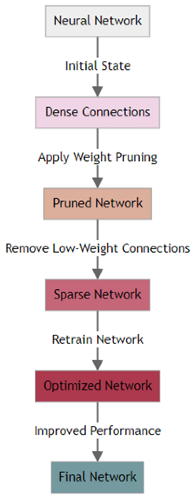
2.2. Model Compression

For deploying audio classification models on resource-constrained devices like the Raspberry Pi 4 and NVIDIA Jetson Nano (Manufactured by NVIDIA, Santa Clara, CA, USA), selecting the right model-compression techniques is crucial to balance performance and efficiency.

2.2.1. Pruning

To compress the model for audio classification we used magnitude pruning and Taylor pruning. Using magnitude pruning and Taylor pruning for model compression offers several benefits, particularly when deploying models on resource-constrained devices like the Raspberry Pi and NVIDIA Jetson Nano. These benefits stem from the ability of these techniques to reduce the model size and computational complexity while maintaining acceptable levels of accuracy. Magnitude pruning significantly reduces the number of parameters in a neural network by eliminating weights with the smallest magnitudes. The equation for magnitude pruning can be expressed as follows:
w = 0 if | w | threshold w otherwise
Here, w is the original weight. w is the pruned weight after applying the magnitude pruning. threshold is a predefined threshold value, and weights with magnitudes below this threshold are pruned to zero. Pruning process is shown in Figure 2.
This leads to a smaller model size, making it more suitable for devices with limited storage, like the Raspberry Pi. With fewer weights to process, the computational load during inference is reduced. This can lead to faster response times, which is crucial for real-time audio classification applications on both the Raspberry Pi and NVIDIA Jetson Nano. Smaller and less-complex models require less power to run, which is beneficial for battery-powered or energy-sensitive applications, a common scenario for Raspberry Pi-based projects. The reduced model size offers more flexibility in deploying complex models on the Raspberry Pi, which might otherwise be infeasible due to memory constraints.
Taylor pruning considers the impact of each weight on the loss function, allowing for a more informed decision about which weights to prune. This often results in a better preservation of model accuracy compared to magnitude pruning.
By focusing on the removal of weights that have the least effect on the model output, Taylor pruning ensures that the computational resources of the NVIDIA Jetson Nano are used more efficiently, focusing on weights that contribute most to the model’s performance. Taylor pruning can be applied to a variety of neural network architectures, making it a versatile choice for different types of audio classification models that might be deployed on these devices. For the NVIDIA Jetson Nano, which has more computational power than the Raspberry Pi, Taylor pruning can effectively balance model complexity and performance, optimizing the use of its GPU capabilities. Below is the equation for Taylor pruning:
L ( w ) L ( w ) + ( w w ) T L ( w ) + 1 2 ( w w ) T H ( w ) ( w w )
A hybrid pruning approach leveraging both magnitude and Taylor pruning techniques can provide a more effective and adaptable solution for model compression. It allows for a nuanced balance between the model size, computational efficiency, and accuracy, which is particularly beneficial in resource-constrained environments or in applications where both speed and accuracy are crucial. Magnitude pruning effectively reduces the model size by eliminating weights with the smallest magnitudes, which are often deemed less important. However, this approach does not always consider the overall impact of each weight on the model’s output. Taylor pruning, on the other hand, evaluates the impact of weights on the loss function, providing a more nuanced view of each weight’s importance. By combining these two methods, a hybrid approach can prune the model more aggressively than magnitude pruning alone (thus reducing the size and computational load) while still maintaining a higher level of accuracy, as it considers the impact of pruning such as Taylor pruning on model performance. Different layers of a neural network might have varying levels of sensitivity to pruning. A hybrid approach allows for a more tailored pruning strategy, where magnitude pruning can be applied more aggressively in layers that are less sensitive, and Taylor pruning can be used in layers where accuracy is more critical. Different neural network architectures may respond differently to pruning. A hybrid approach provides the flexibility to adjust the pruning strategy according to the specific architecture, whether it is a convolutional neural network for image processing or a recurrent neural network for sequence modeling like audio classification. On devices like the Raspberry Pi and NVIDIA Jetson Nano, the reduced model size from magnitude pruning leads to faster inference times and lower power consumption. The careful pruning from the Taylor method ensures that this efficiency does not come at the cost of a significant drop in accuracy. A hybrid approach needs to be implemented iteratively, starting with magnitude pruning to quickly reduce the size and then refining with Taylor pruning to fine-tune the model. This iterative process leads to a more optimized balance between size, speed, and accuracy.

2.2.2. Quantization

8-bit quantization is a highly effective technique for optimizing deep learning models for deployment on devices like the Raspberry Pi and NVIDIA Jetson Nano. It addresses the key challenges of limited computational resources, storage capacity, and power constraints, making it a popular choice for edge computing applications. Quantization reduces the precision of the weights and activations in a neural network from 32-bit floating-point to 8-bit integers. This reduction in bit width leads to a significant decrease in the model size, which is crucial for devices with limited storage capacity like the Raspberry Pi. 8-bit integers are computationally less expensive to process than 32-bit floating-point numbers. This results in faster computation during model inference, which is particularly beneficial for real-time applications like audio or video processing. With smaller data sizes, the memory bandwidth requirement is reduced. This means that data can be transferred more quickly between the memory and the processor, further speeding up the inference process. Most deep learning frameworks support 8-bit quantization, making it a widely accessible technique for optimizing models for edge deployment.

3. Experimental Details

For hardware, the Raspberry Pi and NVIDIA Jetson Nano were used. The Convolutional Neural Network was implemented in PyTorch and the Wavio audio library was used to process the audio files.

3.1. Datasets

The UrbanSound8K [31] dataset was created in 2013 by Salamon, Jacoby, and Bello as part of their research on audio event classification. The dataset is designed to be a resource for researchers and practitioners in the field of audio processing and machine learning. The audio files were recorded in various urban environments, including streets, parks, and residential areas, with a focus on capturing the sounds of everyday life in cities. The UrbanSound8K dataset is a collection of 8000 audio files recorded in various urban environments. Each file is labeled with one of ten different classes, including “air conditioning”, “car horn”, “children playing”, “dog bark”, “drilling”, “engine idling”, “gunshot”, “jackhammer”, “siren”, and “street music”. Each of the 8000 audio files in the dataset is 4 s long and is labeled with one of the 10 classes mentioned earlier. The dataset was created to provide a challenging and diverse set of audio events that can be used to evaluate and compare the performance of different audio classification algorithms.
The ESC-50 [32] dataset is a collection of 2000 environmental sound recordings organized into 50 different classes. The classes include various types of natural sounds, such as water sounds, animal sounds, and weather sounds, as well as man-made sounds, such as vehicle sounds, alarm sounds, and musical instrument sounds. Each sound recording is 5 s long and is annotated with the corresponding class label.
Audio Set [33] is a large-scale dataset of audio events and scenes created by Google. The dataset contains over 2 million 10 s audio clips, representing a diverse range of sounds, including human speech, music, animal sounds, and environmental sounds. Each audio clip is annotated with one or more labels from a hierarchical ontology of over 632 sound event classes, including fine-grained classes such as “saxophone” and “dog bark” as well as broader classes such as “music” and “animal”.

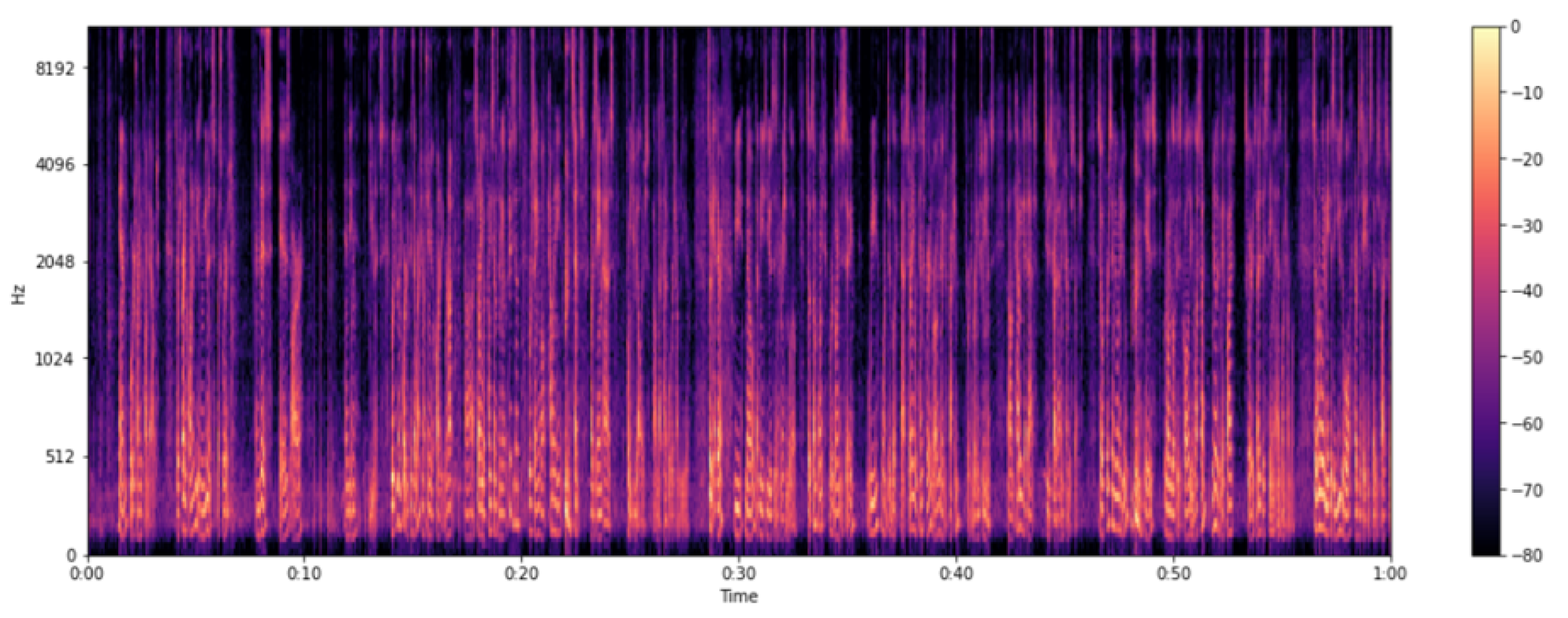
3.2. Data Preprocessing

The ESC-50 dataset comprises a total of 2000 audio samples, each with a duration of five seconds. These samples were recorded at two distinct sampling rates: 16 kHz and 44.1 kHz. The dataset is meticulously organized into 50 distinct and balanced classes, with each class containing 40 individual audio samples. Additionally, the ESC-50 dataset is partitioned into five separate splits, a structure that facilitates the implementation of five-fold cross-validation, thereby aiding researchers in obtaining unbiased and comparable experimental results. By contrast, the UrbanSound8K (US8K) dataset encompasses 8732 labeled audio clips. Each clip, featuring urban soundscapes, has a maximum duration of four seconds and was recorded at a sampling rate of 22.05 kHz. This dataset is categorized into 10 classes. Notably, the US8K dataset is pre-arranged into 10 folds, specifically designed to support 10-fold cross-validation. This arrangement is instrumental in ensuring that the research outcomes are unbiased and comparable, adhering to rigorous academic standards. The network in question is configured to process audio data sampled at 20 kHz, with each input corresponding to a length of 30,225 data points. This length equates to approximately 1.51 s of audio. The decision to downsample the data to 20 kHz was driven by the objective to minimize the input size, reduce the overall model size, and decrease the power consumption. It is noteworthy that based on empirical observations, the performance of the network remains consistent and unaffected when handling audio that has been resampled at this lower rate. This indicates that the reduction in the sampling rate to 20 kHz does not detrimentally impact the network’s ability to process and analyze audio data effectively.
Mel spectrograms (Figure 3), created by mimicking the non-linear response of the human ear to different frequencies, offer advantages over raw audio data. They compress frequency information, capturing essential acoustic features while reducing redundancy. The high-dimensional nature of raw audio data is condensed into a more manageable set of features, aligning with machine learning preferences for lower-dimensional inputs. Mel spectrograms are designed to be perceptually relevant, enhancing performance in tasks influenced by human perception, such as speech-related applications. They also exhibit better noise robustness due to frequency compression and feature extraction, reducing the impact of irrelevant noise. Moreover, the computational efficiency of Mel spectrograms makes them a practical choice by providing a more efficient representation for processing in terms of both memory and computation.

4. Results

In this study, the extraction of low-level features from raw audio data is a critical step, with a particular focus on the zero crossing rate (ZCR). ZCR, a key measure in the analysis of audio signals, quantifies the frequency at which the audio waveform crosses the zero amplitude axis, thereby providing insights into the frequency content of the signal. This metric is integral to various digital signal processing applications, including speech and music analysis, as well as broader audio classification tasks. The utility of ZCR lies in its ability to effectively differentiate between tonal sounds, which exhibit a lower ZCR, and more noisy or percussive elements, characterized by a higher ZCR.
A notable challenge arises when the audio contains significant ‘dead spots’ or segments of minimal amplitude, as these can obscure the distinctive features of the audio, leading to difficulties in classification. To mitigate this issue, the initial step involves the cleansing of audio data by removing dead space, utilizing a technique that involves the application of a signal envelope. The signal envelope, a conceptual curve outlining the extremes of the audio waveform, provides a framework for identifying and excising sections of the audio below a threshold of 20 dB.
For uniformity and computational efficiency, the audio clips were standardized to a fixed frame size. To facilitate the real-time GPU-based extraction of audio features from Mel spectrograms, the study employed Keras audio preprocessors (Kapre). Kapre’s capabilities extend to the optimization of signal parameters in real time, significantly simplifying and enhancing the reliability of model deployment.
In Table 2, the comparison between the audio classification using raw audio and Mel spectrograms is shown. The Mel spectrograms achieve the highest accuracy of 95%.
We have also shown in Table 3 that with the proposed methodology, the experimental result was also better than with many existing models.
Hybrid pruning, combining magnitude and Taylor pruning, offers superior model optimization by balancing the efficient size reduction of magnitude pruning with the precision of Taylor pruning. In Table 4, we can see that hybrid pruning obtained better accuracy than the individual pruning methods. This approach enhances the network performance and generalization while maintaining an optimal level of complexity. It strikes a fine balance between computational efficiency and the retention of crucial network features.
Though we obtained better accuracy for audio classification using pruning techniques, the model size and execution time were smaller using quantization techniques. A comparison between the accuracy and model size is shown in Table 5.
Later, the audio classification model was deployed in the Raspberry Pi4 and NVIDIA Jetson Nano to check the performance. Table 6 shows the results of the accuracy, inference time, and power consumption in the devices.

5. Conclusions

In contemporary applications, edge devices augmented with audio classification capabilities are pivotal in enhancing a myriad of real-world scenarios. In domestic environments, such technologies facilitate the intuitive, hands-free interaction with smart home systems and yield immediate auditory feedback. Within the healthcare sector, these devices play a crucial role in the perpetual monitoring and early diagnosis of conditions like sleep apnea, offering vital, real-time data. Furthermore, in the public safety and industrial domains, their ability to detect auditory cues of distress or mechanical irregularities significantly bolsters emergency responsiveness and operational safety. In our research, it has been observed that the efficacy of audio classification is notably enhanced when utilizing Mel spectrograms as opposed to raw audio data. Particularly in scenarios where accuracy is paramount, Mel spectrograms emerge as the preferred methodology. The significance of audio classification in edge device applications is underscored by its widespread applicability. To facilitate real-world deployment, it is imperative to compress these models efficiently. Our findings indicate that hybrid pruning outperforms singular pruning methods in this context. Additionally, the implementation of quantization techniques contributes to a further reduction in the model size, thereby expediting execution on edge devices.

Author Contributions

Writing—original draft, A.M.; Supervision, M.M. All authors have read and agreed to the published version of the manuscript.

Funding

The research is funded by the NSF I-Corps 21552- National Innovation and the National Science Foundation under Award No. OIA-1946391(DART). Any opinions, findings, and conclusions, or recommendations expressed in this material are those of the author(s) and do not necessarily reflect the views of the National Science Foundation.

Data Availability Statement

Data is contained within the article.

Conflicts of Interest

The authors declare no conflicts of interest.

References

  1. der Mauer, M.A.; Behrens, T.; Derakhshanmanesh, M.; Hansen, C.; Muderack, S. Applying sound-based analysis at porsche production: Towards predictive maintenance of production machines using deep learning and internet-of-things technology. In Digitalization Cases: How Organizations Rethink Their Business for the Digital Age; Springer: Berlin/Heidelberg, Germany, 2019; pp. 79–97. [Google Scholar]
  2. Yun, H.; Kim, H.; Kim, E.; Jun, M.B. Development of internal sound sensor using stethoscope and its applications for machine monitoring. Procedia Manuf. 2020, 48, 1072–1078. [Google Scholar] [CrossRef]
  3. Sharan, R.V.; Moir, T.J. An overview of applications and advancements in automatic sound recognition. Neurocomputing 2016, 200, 22–34. [Google Scholar] [CrossRef]
  4. Xu, W.; Zhang, X.; Yao, L.; Xue, W.; Wei, B. A multi-view CNN-based acoustic classification system for automatic animal species identification. Ad. Hoc. Netw. 2020, 102, 102115. [Google Scholar] [CrossRef]
  5. Stowell, D.; Petrusková, T.; Šálek, M.; Linhart, P. Automatic acoustic identification of individuals in multiple species: Improving identification across recording conditions. J. R. Soc. Interface 2019, 16, 20180940. [Google Scholar] [CrossRef] [PubMed]
  6. Yan, X.; Zhang, H.; Li, D.; Wu, D.; Zhou, S.; Sun, M.; Hu, H.; Liu, X.; Mou, S.; He, S.; et al. Acoustic recordings provide detailed information regarding the behavior of cryptic wildlife to support conservation translocations. Sci. Rep. 2019, 9, 5172. [Google Scholar] [CrossRef] [PubMed]
  7. Radhakrishnan, R.; Divakaran, A.; Smaragdis, A. Audio analysis for surveillance applications. In Proceedings of the IEEE Workshop on Applications of Signal Processing to Audio and Acoustics, New Paltz, NY, USA, 16–19 October 2005; IEEE: Piscataway, NJ, USA, 2005; pp. 158–161. [Google Scholar]
  8. Vacher, M.; Serignat, J.F.; Chaillol, S. Sound classification in a smart room environment: An approach using GMM and HMM methods. In Proceedings of the 4th IEEE Conference on Speech Technology and Human-Computer Dialogue (SpeD 2007), Iasi, Romania, 10–12 May 2007; Publishing House of the Romanian Academy: Bucharest, Romania, 2007; Volume 1, pp. 135–146. [Google Scholar]
  9. Wong, P.K.; Zhong, J.; Yang, Z.; Vong, C.M. Sparse Bayesian extreme learning committee machine for engine simultaneous fault diagnosis. Neurocomputing 2016, 174, 331–343. [Google Scholar] [CrossRef]
  10. Guo, L.; Li, N.; Jia, F.; Lei, Y.; Lin, J. A recurrent neural network based health indicator for remaining useful life prediction of bearings. Neurocomputing 2017, 240, 98–109. [Google Scholar] [CrossRef]
  11. Pacheco, F.; de Oliveira, J.V.; Sánchez, R.V.; Cerrada, M.; Cabrera, D.; Li, C.; Zurita, G.; Artés, M. A statistical comparison of neuroclassifiers and feature selection methods for gearbox fault diagnosis under realistic conditions. Neurocomputing 2016, 194, 192–206. [Google Scholar] [CrossRef]
  12. Liu, J.; Wang, W.; Golnaraghi, F. An enhanced diagnostic scheme for bearing condition monitoring. IEEE Trans. Instrum. Meas. 2009, 59, 309–321. [Google Scholar]
  13. Henriquez, P.; Alonso, J.B.; Ferrer, M.A.; Travieso, C.M. Review of automatic fault diagnosis systems using audio and vibration signals. IEEE Trans. Syst. Man Cybern. Syst. 2013, 44, 642–652. [Google Scholar] [CrossRef]
  14. Malmberg, C. Real-Time Audio Classification onan Edge Device: Using YAMNet and TensorFlow Lite. Ph.D. Thesis, Linnaeus University, Vaxjo, Sweden, 2021. [Google Scholar]
  15. Sharma, G.; Umapathy, K.; Krishnan, S. Trends in audio signal feature extraction methods. Appl. Acoust. 2020, 158, 107020. [Google Scholar] [CrossRef]
  16. Wang, Y.; Wei-Kocsis, J.; Springer, J.A.; Matson, E.T. Deep learning in audio classification. In Proceedings of the International Conference on Information and Software Technologies, Kaunas, Lithuania, 13–15 October 2022; Springer: Berlin/Heidelberg, Germany, 2022; pp. 64–77. [Google Scholar]
  17. Zaman, K.; Sah, M.; Direkoglu, C.; Unoki, M. A Survey of Audio Classification Using Deep Learning. IEEE Access 2023, 11, 106620–106649. [Google Scholar] [CrossRef]
  18. Maccagno, A.; Mastropietro, A.; Mazziotta, U.; Scarpiniti, M.; Lee, Y.C.; Uncini, A. A CNN approach for audio classification in construction sites. In Progresses in Artificial Intelligence and Neural Systems; Springer: Berlin/Heidelberg, Germany, 2021; pp. 371–381. [Google Scholar]
  19. Wang, X.; Han, Y.; Leung, V.C.M.; Niyato, D.; Yan, X.; Chen, X. Convergence of Edge Computing and Deep Learning: A Comprehensive Survey. IEEE Commun. Surv. Tutor. 2020, 22, 869–904. [Google Scholar] [CrossRef]
  20. Murshed, M.S.; Murphy, C.; Hou, D.; Khan, N.; Ananthanarayanan, G.; Hussain, F. Machine learning at the network edge: A survey. ACM Comput. Surv. CSUR 2021, 54, 1–37. [Google Scholar] [CrossRef]
  21. Mohaimenuzzaman, M.; Bergmeir, C.; Meyer, B. Pruning vs XNOR-net: A comprehensive study of deep learning for audio classification on edge-devices. IEEE Access 2022, 10, 6696–6707. [Google Scholar] [CrossRef]
  22. Choudhary, T.; Mishra, V.; Goswami, A.; Sarangapani, J. A comprehensive survey on model compression and acceleration. Artif. Intell. Rev. 2020, 53, 5113–5155. [Google Scholar] [CrossRef]
  23. Krizhevsky, A.; Sutskever, I.; Hinton, G.E. Imagenet classification with deep convolutional neural networks. In Advances in Neural Information Processing Systems; Curran Associates, Inc.: New Paltz, NY, USA, 2012; Volume 25. [Google Scholar]
  24. Taigman, Y.; Yang, M.; Ranzato, M.; Wolf, L. Deepface: Closing the gap to human-level performance in face verification. In Proceedings of the Proceedings of the IEEE Conference on Computer Vision and Pattern Recognition, Columbus, OH, USA, 23–28 June 2014; pp. 1701–1708. [Google Scholar]
  25. Mohaimenuzzaman, M.; Bergmeir, C.; West, I.; Meyer, B. Environmental Sound Classification on the Edge: A Pipeline for Deep Acoustic Networks on Extremely Resource-Constrained Devices. Pattern Recognit. 2023, 133, 109025. [Google Scholar] [CrossRef]
  26. Choi, K.; Kersner, M.; Morton, J.; Chang, B. Temporal knowledge distillation for on-device audio classification. In Proceedings of the 2022 IEEE International Conference on Acoustics, Speech and Signal Processing (ICASSP), Virtual Conference, 7–13 May 2022; IEEE: Piscataway, NJ, USA, 2022; pp. 486–490. [Google Scholar]
  27. Hwang, I.; Kim, K.; Kim, S. On-Device Intelligence for Real-Time Audio Classification and Enhancement. J. Audio Eng. Soc. 2023, 71, 719–728. [Google Scholar] [CrossRef]
  28. Kulkarni, A.; Jabade, V.; Patil, A. Audio Recognition Using Deep Learning for Edge Devices. In Proceedings of the International Conference on Advances in Computing and Data Sciences, Kumool, India, 22–23 April 2022; Springer: Berlin/Heidelberg, Germany, 2022; pp. 186–198. [Google Scholar]
  29. Choudhary, S.; Karthik, C.; Lakshmi, P.S.; Kumar, S. LEAN: Light and Efficient Audio Classification Network. In Proceedings of the 2022 IEEE 19th India Council International Conference (INDICON), Kochi, India, 24–26 November 2022; IEEE: Piscataway, NJ, USA, 2022; pp. 1–6. [Google Scholar]
  30. Kumar, A.; Ithapu, V. A sequential self teaching approach for improving generalization in sound event recognition. In Proceedings of the International Conference on Machine Learning (PMLR), Virtual Event, 13–18 July 2020; pp. 5447–5457. [Google Scholar]
  31. Salamon, J.; Jacoby, C.; Bello, J.P. A dataset and taxonomy for urban sound research. In Proceedings of the 22nd ACM International Conference on Multimedia, Orlando, FL, USA, 3–7 November 2014; pp. 1041–1044. [Google Scholar]
  32. Piczak, K.J. ESC: Dataset for environmental sound classification. In Proceedings of the 23rd ACM International Conference on Multimedia, Brisbane, Australia, 26–30 October 2015; pp. 1015–1018. [Google Scholar]
  33. Gemmeke, J.F.; Ellis, D.P.W.; Freedman, D.; Jansen, A.; Lawrence, W.; Moore, R.C.; Plakal, M.; Ritter, M. Audio Set: An ontology and human-labeled dataset for audio events. In Proceedings of the 2017 IEEE International Conference on Acoustics, Speech and Signal Processing (ICASSP), New Orleans, LA, USA, 5–9 March 2017; pp. 776–780. [Google Scholar] [CrossRef]
  34. Piczak, K.J. Environmental sound classification with convolutional neural networks. In Proceedings of the 2015 IEEE 25th International Workshop on Machine Learning for Signal Processing (MLSP), Boston, MA, USA, 17–20 September 2015; IEEE: Piscataway, NJ, USA, 2015; pp. 1–6. [Google Scholar]
  35. Kim, J. Urban sound tagging using multi-channel audio feature with convolutional neural networks. In Proceedings of the Detection and Classification of Acoustic Scenes and Events, Tokyo, Japan, 2–3 November 2020; Volume 1. [Google Scholar]
  36. Boddapati, V.; Petef, A.; Rasmusson, J.; Lundberg, L. Classifying environmental sounds using image recognition networks. Procedia Comput. Sci. 2017, 112, 2048–2056. [Google Scholar] [CrossRef]
Figure 1. Pipeline of the proposed method.
Sci 06 00021 g001
Figure 2. Pruning.
Figure 2. Pruning.
Sci 06 00021 g002
Figure 3. Mel spectrogram.
Sci 06 00021 g003
Table 1. CNN Architecture.
LayerOperation/Description
Conv2dInput: (1, 1, 30,225)
Filters: 8, Kernel: (1, k); Output: (8, 1, 15,109)
Batch Normalization, ReLU Activation
MaxPool2dMax Pooling, Kernel: (2, 1); Stride: (2, 1); Output: (8, 1, 7554)
AvgPool2dAverage Pooling, Kernel: (2, 1); Stride: (2, 1); Output: (8, 1, 3777)
PermutePermute Dimension Order
FlattenFlatten to 1D Vector
LinearFully Connected Layer, Output: (1, n)
SoftmaxSoftmax Activation for Classification
Table 2. Audio classification comparison between feature extractions by raw audio and Mel spectrogram.
DatasetsRaw AudioMel Spectrograms
ESC-5091%92.7%
UrbanSound8k79%84%
AudioSet90%95%
Table 3. Comparison of our result with the existing results of Mel spectrograms.
NetworksESC50US8k
Pizak-CNN [34]64.50%73.70%
Multi-CNN [35]89.50%-
GoogLENet [36]73%93%
Proposed92.7%84%
Table 4. Comparison between different pruning methods.
Pruning MethodsAccuracy
Weight88%
Taylor88.75%
Hybrid89.25%
Table 5. Comparison between pruning and quantization.
Model CompressionAccuracyModel Size
Original Model92%18.18 MB
Pruning89.25%528 KB
Quantization85.25%157 KB
Table 6. Performance of audio classification on edge devices.
DeviceAccuracyInference TimePower Consumption
Raspberry pi485%3.89 s/it7 W
NVIDIA Jetson Nano88%2.12 s/it10 W
Disclaimer/Publisher’s Note: The statements, opinions and data contained in all publications are solely those of the individual author(s) and contributor(s) and not of MDPI and/or the editor(s). MDPI and/or the editor(s) disclaim responsibility for any injury to people or property resulting from any ideas, methods, instructions or products referred to in the content.

