Spatiotemporal Analysis of Human Mobility in Greater Tokyo Area Using Hourly 500 m Mobile Spatial Statistics from 2019 to 2021

Abstract

Spatiotemporal evaluation of human mobility is crucial to deepen and broaden the understanding of drivers and mechanisms behind urbanization. In this study, daytime human mobility was quantified based on the inflow and outflow of population in 500 × 500 m spatial grids using a processed version of the hourly DOCOMO Mobile Spatial Statistics (MSS) dataset. Using K-means clustering of the temporal mobility values over the Greater Tokyo Area, five typical diurnal patterns representing distinguishable intensities of diurnal human mobility over weekdays and weekends were identified. Mapping their spatiotemporal changes from the period of January 2019 to December 2021, a different perspective on regional human mobility was explored. These include the influence of the COVID-19 pandemic on human mobility, the relationship between human mobility and locations of public infrastructures, and a large-scale human mobility across central and peripheral areas inside the large megacity.

1. Introduction

Cities are drastically changing worldwide. In the last decade, the population in urban areas has exceeded half of the world’s population and has been found to be rapidly increasing [1]. Due to this rapid growth alongside the hazards arising from climate change and pandemics (e.g., COVID-19), risks are expected to increase in urban areas in cities. As urbanization continues to invade the natural environment [2] and affects the human population, a deeper understanding of its important driver, human mobility, is becoming increasingly crucial.

Human mobility, defined as the movement of individuals or groups of individuals, indicates the unique state and development of cities [3,4]. Beyond its basic definition, the level of human mobility can imply drivers of social phenomena, the state of economies, and the effectiveness of policies [5]. Its further investigation enhances our understanding of various socio-economic, health, and environmental aspects, such as social interactions [6,7,8], economic activities [9], migration [10], traffic flows [11], epidemic spread [12,13], and disaster resilience [14].

As a complex phenomenon, human mobility has been investigated using multiple approaches [15]. Individual-level models, such as Lévy flight [16] or preferential return [17], as well as population-level models like the gravity law [18], radiation model [10,13], and visitation law [19], are among them. Other works have employed data-driven approaches, such as network analysis [20,21,22] and machine learning techniques [23]. A wide array of data types has been utilized to represent mobility, including census and survey data [10,13,22], dollar bills [16], call and text records [7,13,14,17,22,24], GPS data [21], and mobile phone location information [7,11,19,20,23,24,25,26].

Most human mobility studies focus on the travel or trip behavior of the population. The metrics often used to explain mobility in these studies include trip distance, trip duration, trip destination, number of visited locations, and visitation frequency [7,10,11,16,17,18,19,22,24]. Although these studies have significantly contributed to the understanding of mobility, a broader and alternative perspective of human mobility is still needed. In recent years, an alternative approach to reconstructing mobility profiles at multiple locations over an area is gaining traction due to the emergence of high-resolution gridded population estimates. Studies that utilize such temporal profiles often interpret them as the usage of public space or the flow of population in an area. For example, Ref. [27] used smart card data along with Twitter data to find temporal profiles of urban vitality in areas surrounding train stations in London, England. They suggested that similar human mobility patterns can be observed based on area characteristics, location, and associated transport types. The authors of [28] extracted temporal profiles from Google Maps busyness data at 136 high-human-mobility areas in Ankara, Türkiye. They then analyzed the influence of built environments in the areas relevant to the found temporal profiles. The researchers of [23] utilized big data concerning weekly activity patterns for non-residential “point-of-interest” locations in the United States of America to obtain fine-scale human mobility from 2019 to 2020. Through their usage of the temporal profiles, they were able to uncover the effect of COVID-19 on changing human mobility dynamics in the country. Further, Ref. [29] employed a slightly different approach to highlight the contribution of COVID-19 to the nationwide train demand loss in Japan using mobile spatial statistics. Instead of direct human mobility, they were able to derive temporal profiles of reduced station vitality. Using the same dataset, Ref. [30] identified temporal profiles of variation in the presence of people with respect to the average of 500 m grids in Kyoto. They were able to identify spatial zones in order to measure the effect of pre-COVID-19, COVID-19, and post-COVID-19 on nighttime activity over a period of three weeks. Despite all of these advancements, an overall and explicit mapping of typical temporal human mobility profiles (e.g., hourly daytime variations) fully covering wider regions over longer periods is still missing. Obtaining an overall perspective has significant implications for developing a deeper understanding of human mobility across spatial scales, with practical multi-disciplinary significance.

To address this research gap, this study investigated human mobility at both the intraregional scale and neighborhood scale (e.g., 500 m spatial resolution) over a large megacity, specifically the Greater Tokyo Area, Japan, from 2019 to 2021.

The Greater Tokyo Area (henceforth, Tokyo) was selected for this study as it has been the world’s largest megacity in recent years, with an urban population of approximately 38 million people [31,32]. A unique characteristic of Tokyo is its usage of trains as the primary mode of transportation, accounting for 51% of the transport mode share in 2018 [33] as residents travel to different destinations based on their trip purposes. Despite its uniqueness, the general diurnal behavior of people within Tokyo aligns with those commonly observed in other large cities. The standard working days (weekdays) run from Monday to Friday, while Saturdays and Sundays are generally considered non-working days (weekends). Businesses, schools, and public offices usually start at 09:00 and end at 18:00 on weekdays [34]. Commercial establishments, such as department stores, generally open later around 10:00, and close between 20:00 and 23:00. Throughout the year, daylights saving time is not observed. While these descriptions represent general trends, the majority of the places have slight variations in operating hours, with some exceptions having significantly different schedules.

Both intraregional and neighborhood scales were investigated to inspect the distinct behaviors emerging on different scales [6,35]. At the intraregional scale, the general large-scale mobility between central areas of concentrated human activities and peripheral residential areas can be identified. At the neighborhood scale, a population’s mobility and behavior can be more diverse depending on the locations in question and their functional characteristics such as workplace and services [4,36]. Consequently, this work also extends further to investigate the relationship between public service infrastructures and neighborhood-scale human mobility.

The above investigation was achieved through temporally varying gridded estimates of the population. This work leveraged the DOCOMO Mobile Spatial Statistics (MSS) dataset [37], which provides real-time, hourly population data that have spatial and temporal resolutions of 500 m. MSS has been validated and utilized in aforementioned mobility studies [29,30], disaster-related studies [38,39,40,41], COVID-19 impacts [8,29,30,42,43,44,45], and commercial applications.

In this work, nationwide MSS data were acquired from 2019 to 2021, which also included the early stages of the COVID-19 pandemic. Not only the large-scale patterns in human mobility under usual conditions, but also the temporal variations under unexpected events such as crises and disasters, are investigated in this context. Numerous studies have investigated and confirmed these impacts, particularly examining how COVID-19 and its control measures affected human mobility [8,20,26]. For instance, one study found that reduced social distancing following the relaxation of control measures led to a higher risk of another outbreak [25], while another observed shifts in temporal patterns, such as morning activities starting later after the pandemic [23]. The COVID-19 impacts using the MSS data in Japan were analyzed at the intracity level [8,42,44], the intercity level [43,44,45], and over a period of less than one year [8,42,45]. We contribute to the above works by investigating human mobility and its spatiotemporal changes with respect to the COVID-19 pandemic on both the intraregional scale and neighborhood scale over longer periods.

With the above motivations, the objectives of the research are summarized as follows.

• To elucidate weekday–weekend mobility patterns at the neighborhood scale within Tokyo from 2019 to 2021 using a daytime human mobility index derived from mobile phone statistics.
• To investigate the spatial relationship between the mobility patterns and public infrastructures.
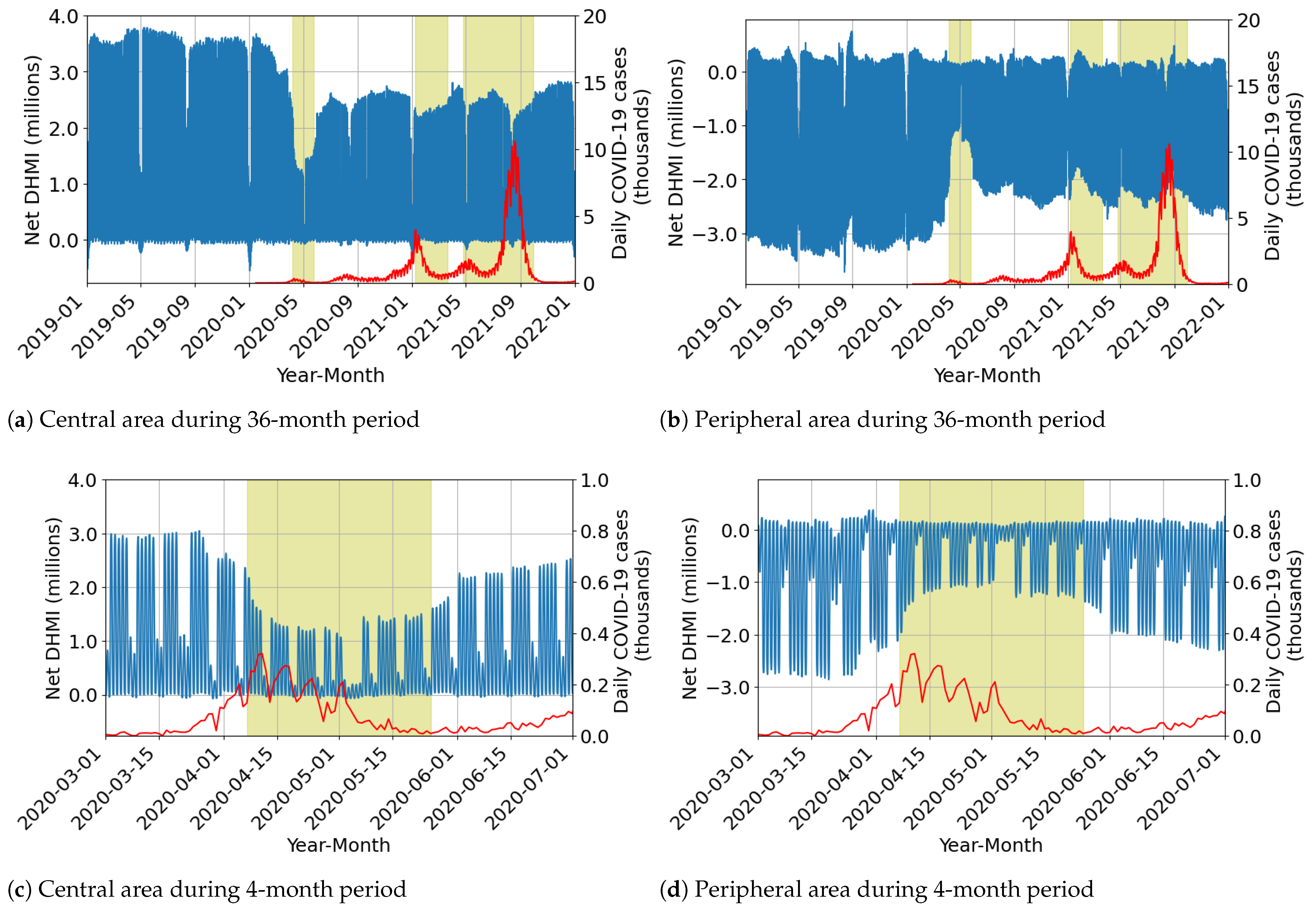
• To investigate central–peripheral human mobility in Tokyo from the established human mobility index.
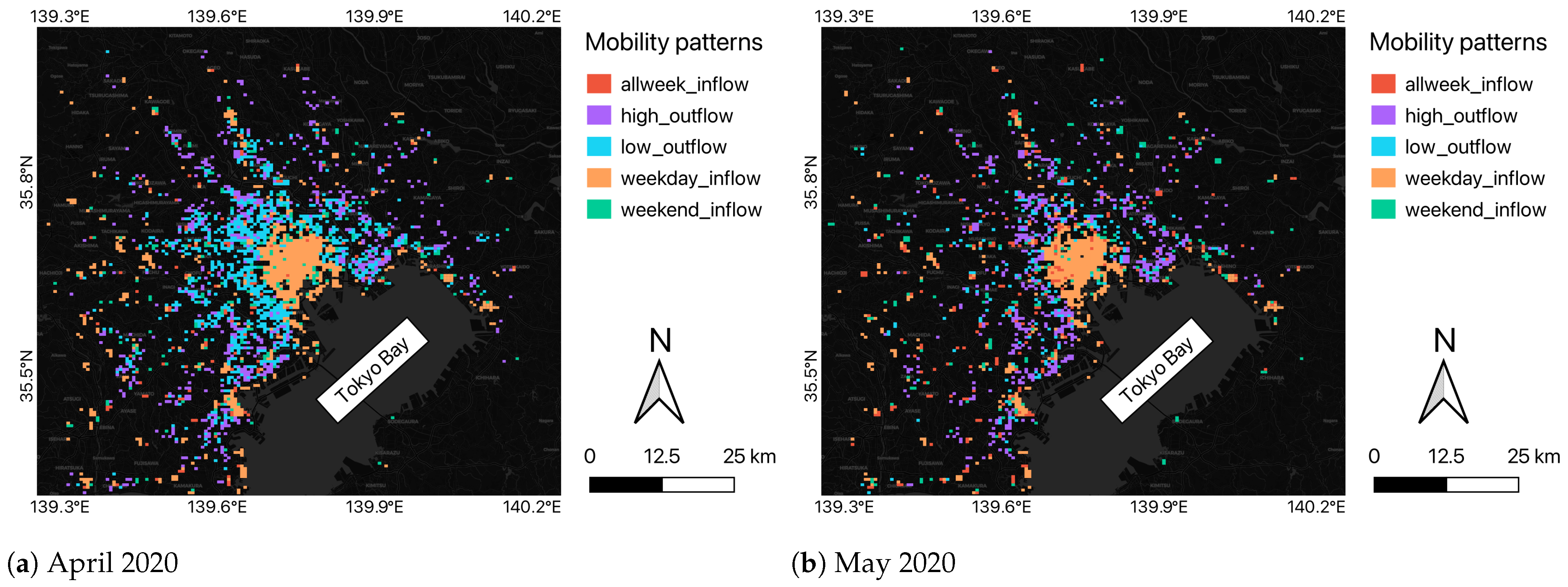
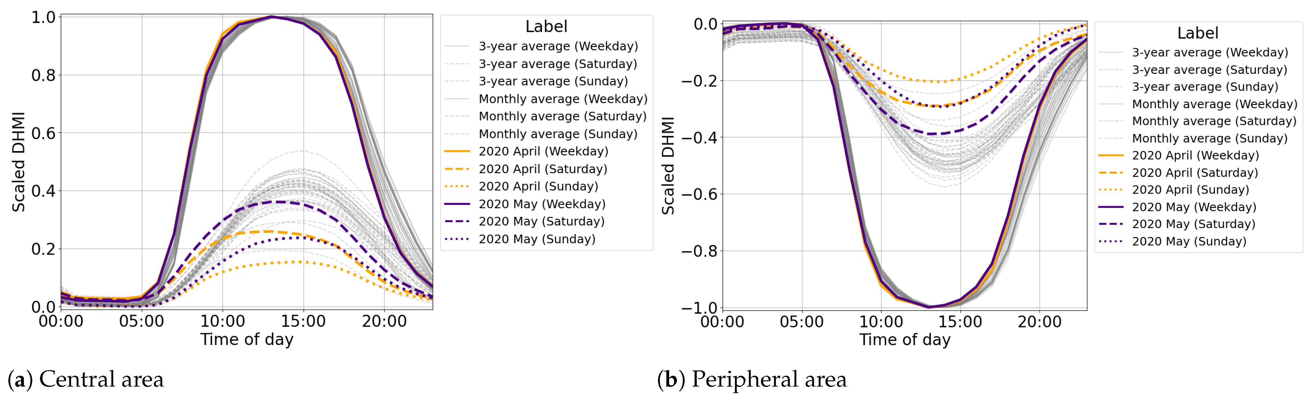
• To demonstrate and evaluate the spatiotemporal changes of human mobility and its patterns during the period surrounding the COVID-19 lockdown in Tokyo.

The work consists of three main parts. First, the classification of human mobility patterns is discussed in Section 2.1 and Section 3.1, which aim to identify typical mobility patterns at a 500 × 500 m grid scale. Second, the quantitative infrastructure spatial analysis, covered in Section 2.2 and Section 3.2, discusses the relationship between the identified mobility patterns and ten public facilities. Third, the capability of the approach to delineate between central and peripheral areas as a function of human mobility are discussed in Section 2.3 and Section 3.3. In line with the three main parts and the study period, the influence of the COVID-19 lockdown is also investigated.

2. Methodology

A diagram of the research framework is shown in Figure 1. The procedure for spatially classifying human mobility patterns from the MSS data for a specified month is explained in this section. Furthermore, procedures to relate the derived classification patterns with infrastructure locations are discussed, followed by the process of estimating human mobility across Tokyo’s central–peripheral boundaries determined from the mobility patterns. The datasets are mentioned in the last sub-section.

2.1. Spatiotemporal Patterns of Human Mobility in Region

This section explains the procedure for finding the typical human mobility patterns from the MSS data using a machine learning technique, K-Means clustering (Figure 2).

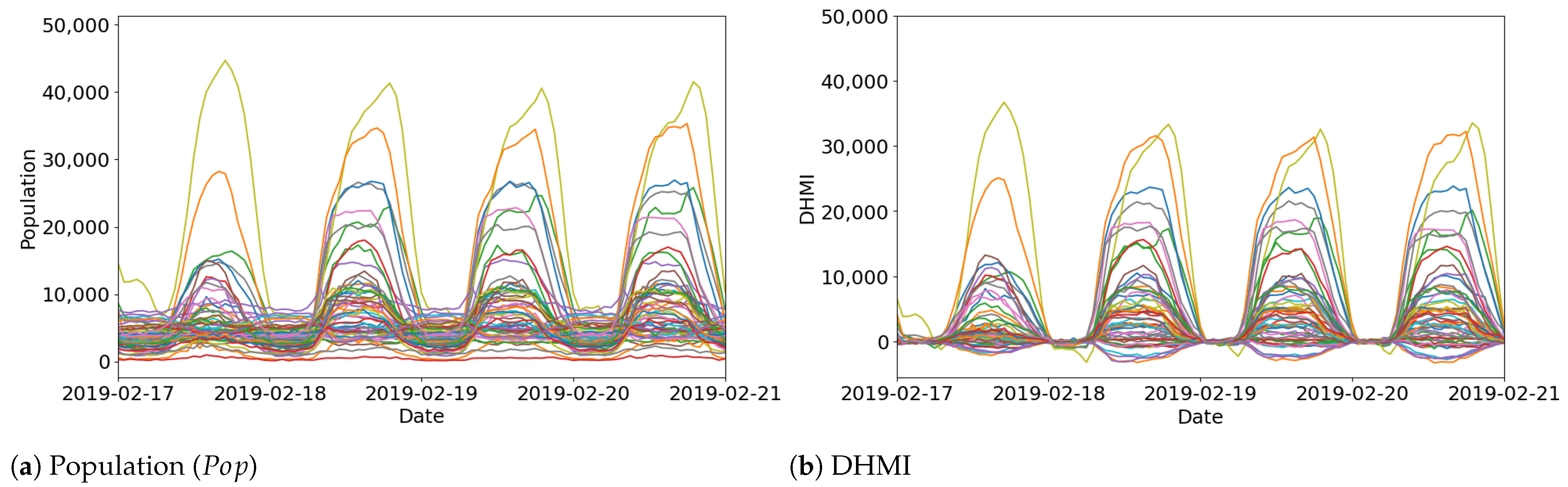
2.1.1. Daytime Human Mobility Index

This work mainly focuses on human mobility during the day. To quantify this, a daytime human mobility index (DHMI) is introduced. DHMI is defined as the local deviation of a local population ($Pop$) of an area from the same area’s residential population ($ResPop$) in a specific time frame (e.g., 1 month). This index can be calculated using Equation (1).

$$\mathrm{DHMI}(G,m,d,t)=Pop(G,m,d,t)-ResPop(G,m)$$

(1)

where G, m, d, t, $Pop$, and $ResPop$ correspond to the grid position, the month, the date, the hour of the day, the local population, and the residential population, respectively.

$ResPop$ was estimated by computing the median of the grid-level population at the local hours of 00:00 to 05:00 (Equation (2)), a period when most individuals are asleep and public transportation is not operating. $ResPop$ was calculated for each month separately to prevent outliers, to capture seasonal variability in residents, and to consider the uncertainties in the MSS-estimated population count [37].

$$ResPop(G,m)=\mathrm{med}\left\{Pop\right(G,m,d,t)\mid (t=[0,1,...,5]\left)AND\right(d\in m\left)\right\}$$

(2)

With each line corresponding to a distinct grid belonging to the district of Shibuya, Figure 3 demonstrates the usefulness of the DHMI and the assumed definition for $ResPop$. The 4-day variations of $Pop$ (Figure 3a) and DHMI (Figure 3b) are illustrated. DHMI adequately captured the timings of population inflows and outflows during the daytime for all grids relative to their respective $ResPop$. Mainly representing the daytime mobility, the DHMI values were approximately 0 from 00:00 to 05:00 local time.

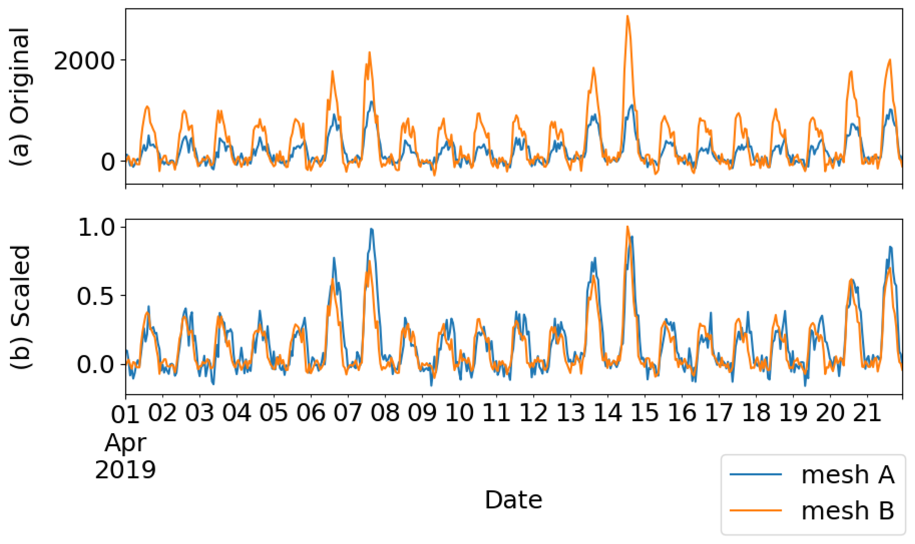
2.1.2. DHMI*: Scaled DHMI

The DHMI was further processed to be used in the classification of various patterns of daytime human mobility (Section 2.1.3). Although human mobility in most grids converges due to significant reductions in mobility during nighttime, varied peak magnitudes of DHMI during the daytime were apparent from one grid to another. To neglect the variability, the DHMI of each grid was scaled by dividing it by the corresponding grid’s monthly maximum DHMI (Equation (3)). The scaled DHMI (i.e., DHMI*) ranges from $[-1,1]$.

$${\mathrm{DHMI}}^{*}(G,m,d,t)={\displaystyle \frac{\mathrm{DHMI}(G,m,d,t)}{\underset{d,t\in m}{max}\left(\right|\mathrm{DHMI}(G,m,d,t)\left|\right)}}$$

(3)

The above scaling eliminated the differences in peak magnitudes across grids while still preserving the levels of mobility. This later allowed the classification algorithm to measure similarity purely in terms of mobility patterns despite the difference in baseline $ResPop$ levels. For example, Figure 4 shows the comparison between (a) DHMI and (b) DHMI*. The visual resemblance between the two example grids became more pronounced. Thus, grids with similar or analogous characteristics could be observed more clearly. A limitation of this work’s approach for detecting mobility patterns was that only grids with a maximum absolute DHMI higher than 1000 could be included due to unstable and incoherent fluctuations appearing for grids having values lower than this threshold. In other words, random inspections of the DHMI* of grids having a maximum absolute DHMI less than this threshold tend to generate extremely large values due to the small denominator values. Grids of this nature are usually found at non-populated locations or locations with extremely low residential populations. In the Greater Tokyo Area, the number of 500 m grids within the prefectural boundaries of Chiba, Saitama, Kanagawa, and Tokyo are 20,319, 14,569, 9590, and 8696, respectively. While the value is proportional to the geographical area occupied by each prefecture, not all of these grids are habitable. By applying this threshold for absolute DHMI, it is possible to identify grids within those prefectures with consistent human mobility and activity. This turned out to be 760, 743, 1350, and 2475, for Chiba, Saitama, Kanagawa, and Tokyo, respectively. These numbers highlight the remarkable concentration of population and anthropogenic activities in Tokyo, despite its relatively smaller geographical size.

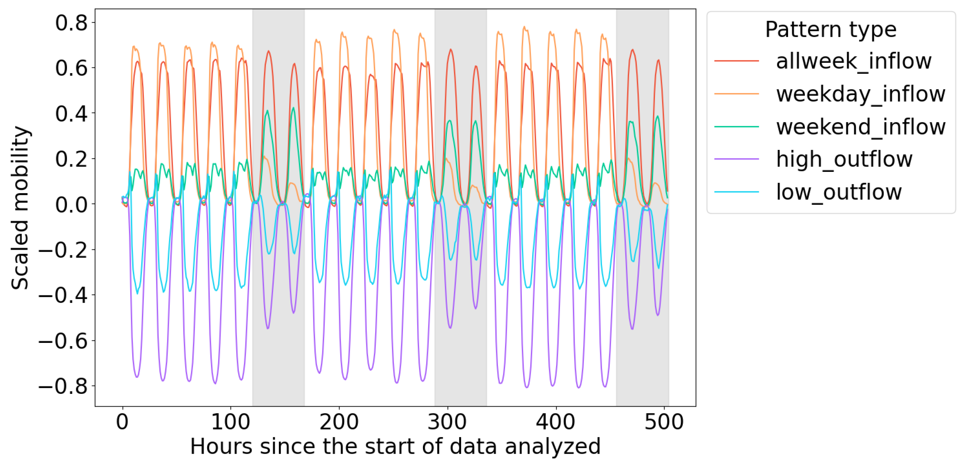
2.1.3. Classifying Mobility Patterns

The classification algorithm used in this research was the K-Means clustering algorithm [46]. K-Means clustering is an unsupervised machine learning method that groups unlabeled data together based on their similarity or closeness, given the number of groups (K). This algorithm groups the data points without requiring prior labelling or predefining target groups. This enables unbiased and automized extraction of common patterns directly from the data. This research used this algorithm to extract prevalent patterns of human mobility that were common across many grids. The process was initiated by randomly selecting K points as the centers and assigning the rest to their closest center. Then, new centers were computed as the average of each group, and the points were reassigned to their closest new center. This process was repeated until a stable grouping result was acquired. Since the mobility data of each location are time-dependent, the measure of distance for determining similarity was based on evaluating the Euclidean distance from the time series of human mobility for each grid. Tslearn Module Version 0.6.3 [47] in Python was used to generate this. Throughout the manuscript, “classification” or “patterns” will be mentioned instead of “clustering” to avoid confusing the word “cluster” with its usage in land use and urban studies [48].

Given two discrete time series data of DHMI*, A and B, their Euclidean distance for time series D was computed using Equation (4).

$$D(A,B)=\sqrt{\sum _{i=1}^n{(a_i-b_i)}^2}$$

(4)

where i refers to the discrete values for each time step. The choice of Euclidean distance over other commonly used measures for time series distance, such as the Dynamic Time Warping [49], was mainly to ensure that the distance is calculated for the same specified discrete time.

The algorithm was applied to DHMI* for each month to consider monthly changes in the mobility pattern over the region. Each month’s data comprise 21 days starting from the first Monday of the month. This was the case to ensure a consistent sequence of weekdays and weekends for each month. Furthermore, the algorithm was trained using April 2019 data because this was the first month within the scope of analysis that did not contain any national holidays within the 21-day period. Various numbers of classification groups (K) were tested to find the most representative and logical mobility patterns. As will be inferred in the discussion of the estimated mobility patterns, $K=5$ was set.

2.2. Quantitative Infrastructure Spatial Analysis

This section explains the procedure for relating the monthly human mobility patterns with various infrastructures (i.e., public facilities and schools) and their geolocations (Figure 5). The details of the infrastructure data and the specific infrastructural types utilized in this study are mentioned in Section 2.4.2.

2.2.1. Data Preprocessing

Infrastructure data were spatially matched [4] with the derived mobility patterns (Section 3.1.2). Given the unique social functions and services of each piece of infrastructure, it is hypothesized that different relationships between human mobility patterns and infrastructure types may exist. Both data have geospatial attributes in vector format: Points for infrastructure data and Polygons (grids) for mobility patterns. The spatial matching was performed by using the “sjoin” function of the Geopandas Module Version 0.10.2 [50] to indicate which grid of the mobility patterns contained each infrastructure. Through this, each grid may be evaluated for the presence of each infrastructure type. Subsequently, the grids can be categorized based on the combinations of their corresponding mobility patterns and the presence of infrastructure (i.e., combination of weekday_inflow mobility pattern and police station infrastructure). By compiling the categorization result and counting the number of grids in each category, a frequency table was constructed (see Appendix A,

Table A1. Grid count comparison for all infrastructures.

	Mobility Patterns
Public	Inflow			Outflow
Infrastructure Types	Allweek	Weekday	Weekend High	Low
Reference	526	796	657	2955	394
Police station	33	62	16	73	14
Municipal office	34	27	12	10	7
Child welfare facility	45	99	55	484	83
Elderly welfare facility	87	91	73	370	58
Fire department	42	71	37	181	34
Hospital	119	122	68	277	53
High school	38	102	45	179	50
Library	51	49	46	166	47
Post office	207	228	144	784	142
University	18	124	25	14	21

).

2.2.2. Quantitative Infrastructure Spatial Analysis

Because of its nonparametric characteristics and the lack of a requirement of equal variance, the Chi-square test of independence [51] was used to conduct hypothesis testing to investigate the relationship between infrastructure and mobility patterns. This is typically used to evaluate the significance of the difference between a reference control group and a treated group to determine the association between variables in a bivariate analysis. In this study, the null hypothesis was that a specified infrastructure does not relate with its immediate surrounding’s human mobility patterns. Rejecting this null hypothesis indicates a statistically significant association between the infrastructure type and its surrounding human mobility patterns. Three possible explanations for this association are proposed as follows: (1) its location was decided by society because of the compared human mobility; (2) that the specified infrastructure influences the compared human mobility, or (3) an unexplored confounding variable exists that influences both the specified infrastructure and its compared human mobility. This investigation was mainly conducted for April 2019. This was because Tokyo’s mobility during that time showed regular mobility fluctuations throughout the 21-day period, and the mobility patterns were generally unchanged with the exception of the lockdown period. This is discussed further in Section 3.1.2.

Although the Chi-square test requires each entry in the table to be represented as frequency or count, the table in Section 3.2 is presented as percentages of total grid count in each row instead. This was carried out to simplify the comparison. The frequency table used for hypothesis testing calculations is included in Appendix A.

2.3. Central–Peripheral Comparative Analysis

In this section, Tokyo was separated into two areas: central and peripheral areas (Figure 6). The central area functions as the downtown area with intense human activities, while the peripheral area consists mainly of residents. This assumption was based on the flow directions of human mobility, namely, inflow and outflow. As will be discussed in Section 3.1.1, individuals likely vacate their residences during the daytime to do business within commercial centers. Thus, this comparative analysis was conducted to investigate the large-scale mobility characteristics between the central area and the peripheral area.

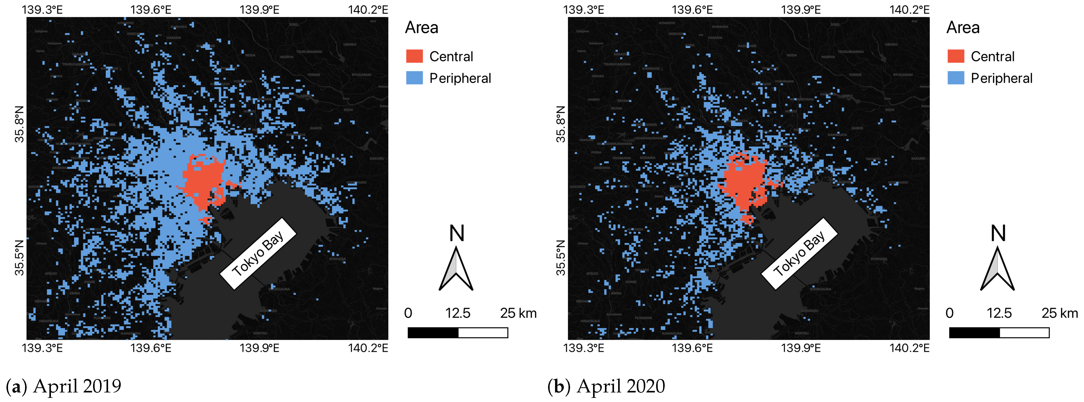
2.3.1. Detection of Central–Peripheral Boundaries

The result of mobility patterns from Section 3.1.2 was used to determine the boundary of the two areas. Initially, mobility patterns were reclassified into broader patterns of inflow and outflow based on their direction of mobility. An example of the reclassified map in April 2019 is illustrated in Figure 7.

Subsequently, the central area was identified by selecting the biggest cluster of inflow. This process was repeated for each month from January 2019 to December 2021. Then, the final boundary (Figure 8) was created by taking the union of the central areas of 36 months without considering possible seasonal changes or abnormalities for simplicity.

Upon closer inspection, the identified central area did not uniformly cover the entire region. Instead, certain parts within the boundary exhibited outflow of population throughout the analytical period. Simple visual investigation revealed that these areas correspond to established residential zones. Consequently, these grids were not included in the central area due to their distinct characteristics aligning more closely with residential areas. Notably, these characteristics included the prevalence of low-rise housing and the absence of high-rise structures and large-scale infrastructure.

After the central area was identified, the peripheral area was designated as the grids that were not included in the central area. The peripheral areas varied for each month depending on the maximum absolute DHMI. Some grids had lower maximum absolute DHMI than the threshold of 1000 in certain months. Consequently, the peripheral area varied for different months. Figure 9 shows a clear example of the comparison of peripheral areas between April 2019 (a typical month) and April 2020 (a month in which Tokyo was under the state of emergency due to COVID-19).

The estimation of a central–peripheral boundary mainly from high spatiotemporal human mobility information presented an added value for mapping mobility patterns. Because of the hourly records covering three years, it became possible to investigate the spatiotemporal changes in these boundaries. These include the changes in the long-term net DHMI and the monthly diurnal DHMI profiles for large-scale mobility.

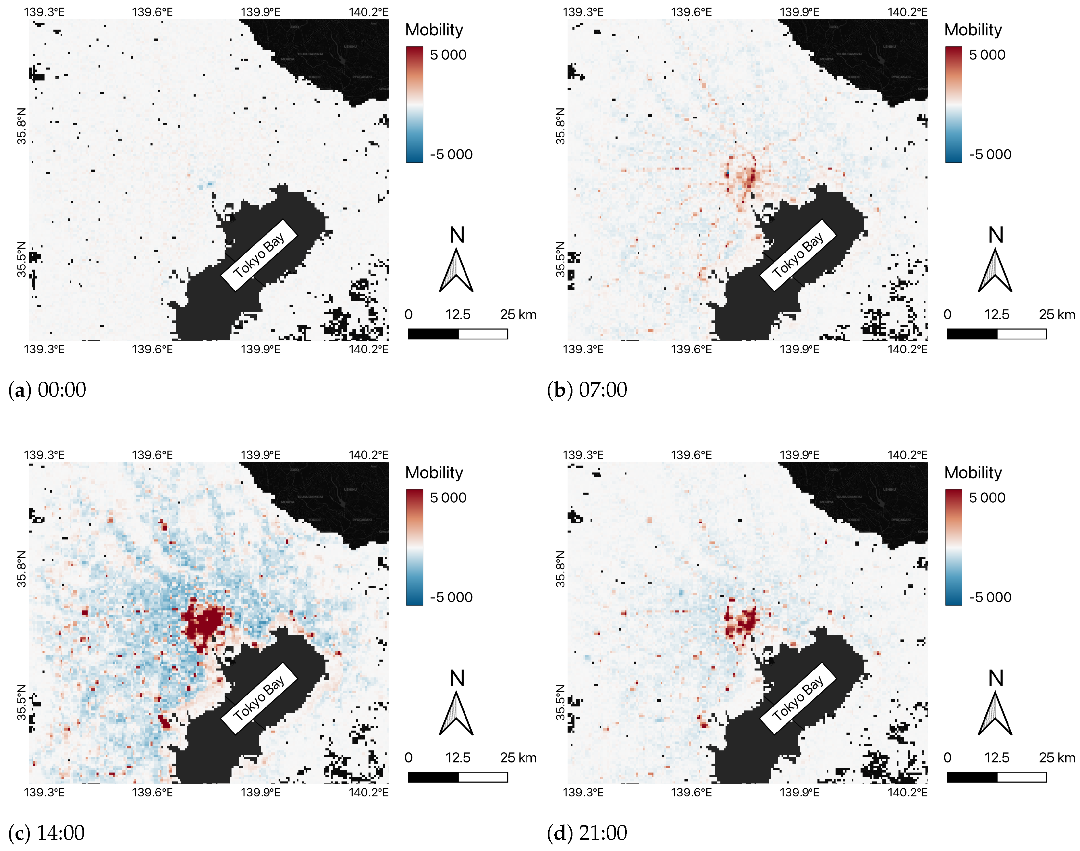
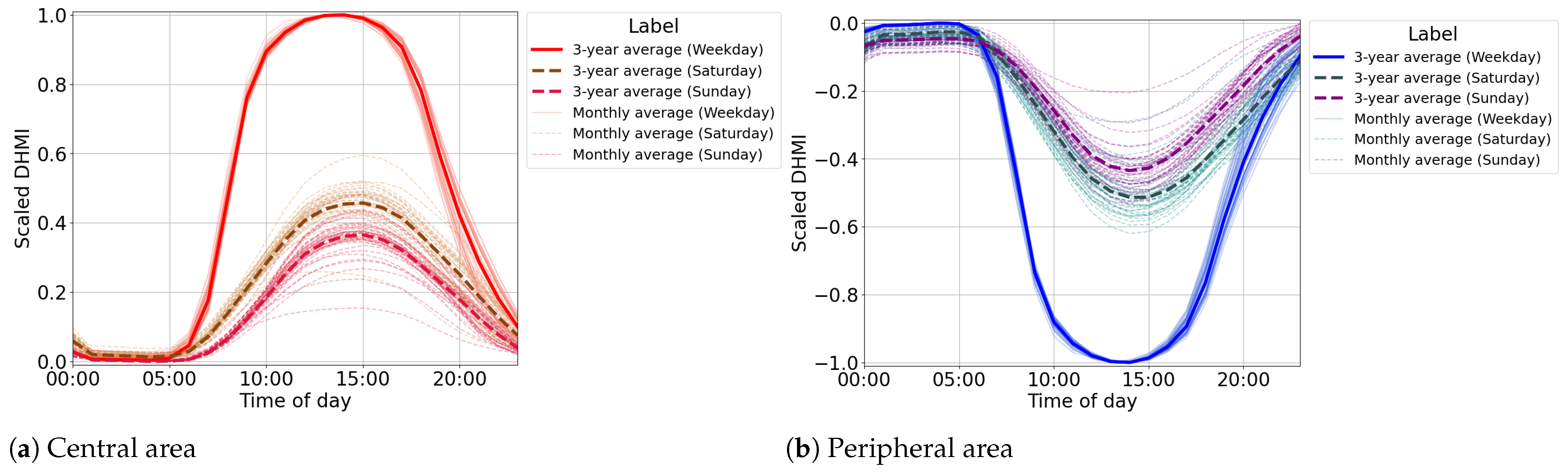
2.3.2. Diurnal Mobility Profile

The net DHMI of large-scale mobility could be found by taking the sum of mobility within central and peripheral areas. Thereafter, the average of net DHMI was calculated for each hour of the day to obtain the representative 24 h diurnal mobility profiles. This calculation was performed monthly over the entire 36-month analysis period to examine variations due to seasonality or extreme events. Finally, MinMaxScaler from the scikit-learn module Version 1.0.1 [52] was applied in order to scale the diurnal profile to the range of $[0,1]$. The scaling was performed to weekdays and weekends together in order to highlight their differences in mobility behaviors. Although the found human mobility patterns in Section 3.1.2 could also be used for the diurnal mobility profiles, they represented smaller-scale mobility at the neighborhood level and had more complexity.

2.4. Datasets Used in This Study

2.4.1. DOCOMO Mobile Spatial Statistics

The MSS dataset is a statistical estimation of Japan’s population provided by NTT Docomo, Inc. [37]. The population estimates in MSS account for Japanese and foreign residents, but does not factor in foreign tourists. The MSS dataset was derived from de-identified operational data collected from the mobile terminal network. The dataset was statistically constructed on an hourly basis by aggregating the count of active mobile terminals within a specific geographic area during the observation period. Subsequently, the count was divided by the presence rate of NTT DOCOMO users to take nonusers into account and estimate the actual population. The presence rate was defined as the proportion of NTT DOCOMO users relative to the actual population that had the same characteristics in terms of gender, age, and address. Thereafter, these estimations were reaggregated into predefined regional 500 m grids [53] for ease of application. In this research, the analysis focuses on the Greater Tokyo Area (i.e., four prefectures including Tokyo, Chiba, Kanagawa, and Saitama) from 2019 to 2021.

2.4.2. Infrastructure Data

Locations of infrastructure [54] were obtained from the publicly available digital land information provided by Japan’s Ministry of Land, Infrastructure, Transport, and Tourism (MLIT). The dataset contains infrastructure names, types, and representative point coordinates of their locations. Although the source has a large data coverage for various facilities, a list of ten public facility types were chosen for this study based on their importance and functions in urban society, namely, Police station, Municipal office, Child welfare facility, Elderly welfare facility, Fire department, Hospital, High school, Library, Post office, and University. Even though the latest available dataset was publicized in 2006, the relevant infrastructure has not undergone significant changes; thus, we assumed that it has remained mostly the same in the last two decades.

3. Results and Discussions

This section describes the main findings of the work in line with the research objectives. It begins with a discussion on the estimated daytime human mobility and its derived classification over the Greater Tokyo Area. This is then followed with an evaluation of the relationship between the spatiotemporal patterns and ten public infrastructure types. Using the net DHMI and the diurnal profiles of human mobility, the intraregional mobility in central areas and peripheral areas is discussed further. At relevant sections, the influence of COVID-19 on human mobility is also discussed.

3.1. Classification of Human Mobility Patterns

3.1.1. Daytime Human Mobility

As shown in Figure 10, the estimated residential population ($ResPop$) matches with the common description of residential populations for most cities. Here, the spatial distribution of the estimated residential population decreases with increasing distance from the city center with extensive branches tracing along major transportation networks. As a characteristic of most large capital cities, a notable drop in the estimated residential population is apparent at the core. At the city center, offices and commercial establishments are prominent and partially influential in driving up land or residential prices. These distinctive characteristics remained consistent across the 36-month analysis period, indicating a stable distribution of the estimated residential population without significant change over time.

Human mobility generally follows a consistent daily pattern. An illustration of human mobility at 00:00, 07:00, 14:00, and 21:00 on 15 April 2019 is presented in Figure 11. The absolute value of DHMI started near zero during the night, increased steadily until midday (as people go out), and then decreased in the late evening (as people return home). The sign (i.e., positive and negative) of DHMI represented the direction of mobility. Positives value indicated inflow, while negative values indicated outflow of people. However, the magnitude and timing of these movements varied slightly for each month, as discussed further in Section 3.3.2.

Spatially, the central area attracted the highest density of people during the daytime, as shown in Figure 11c. Other clusters of population inflow corresponded to smaller commercial centers or attractions, such as Yokohama City. Conversely, areas with population outflow were predominantly residential neighborhoods with a high estimated residential population, as seen in Figure 10.

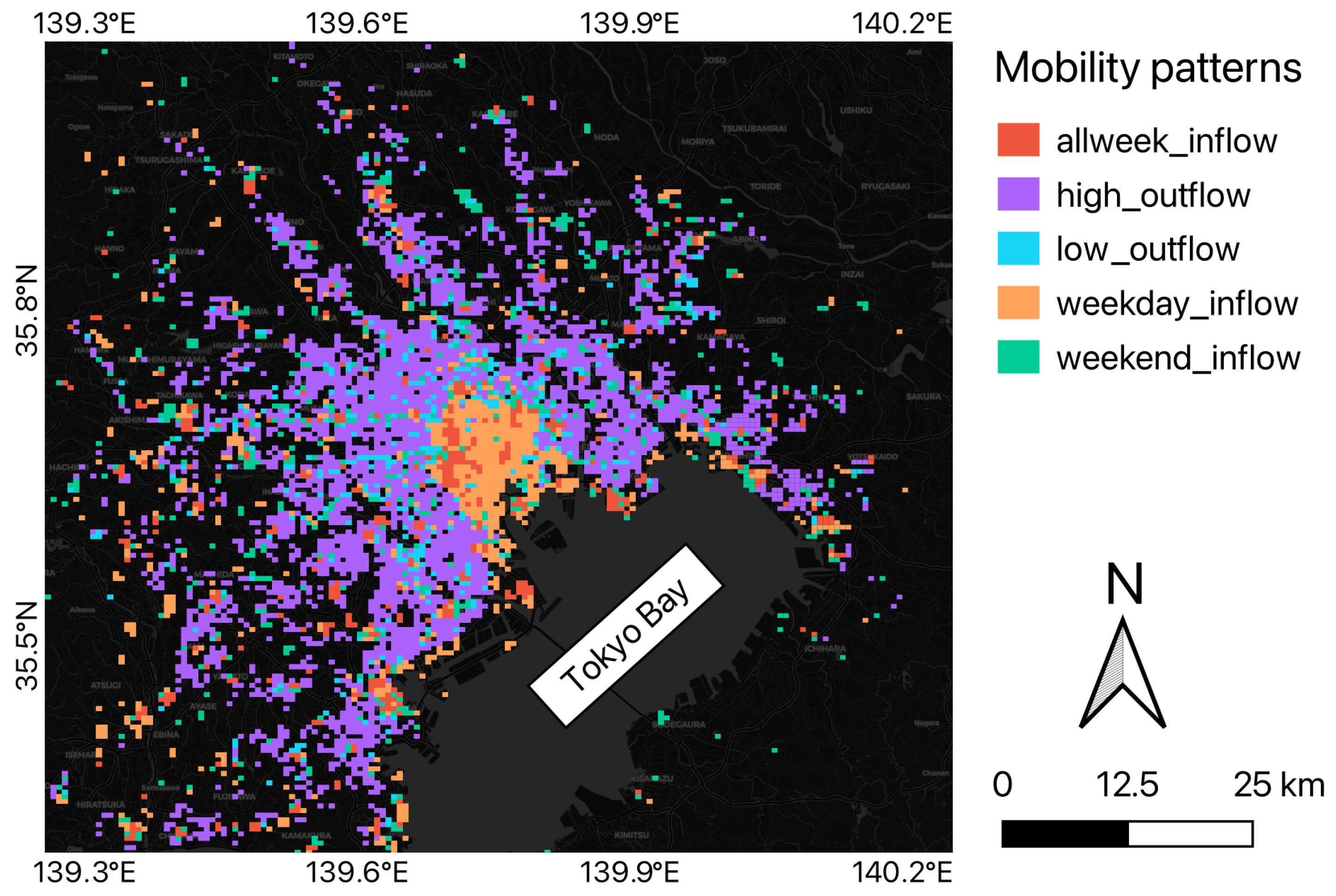
3.1.2. Human Mobility Pattern

Human mobility patterns were classified into five distinct categories: three inflow patterns and two outflow patterns, as illustrated in Figure 12. The three inflow patterns consisted of weekday_inflow, weekend_inflow, and allweek_inflow. These patterns differed in the magnitude of DHMI between weekdays and weekends. Weekday_inflow has a higher inflow of people during weekdays than on weekends. In contrast, the weekend_inflow pattern shows a lower inflow during weekdays compared to weekends. The allweek_inflow pattern maintains a constant inflow of people throughout the entire week. On the other hand, outflow patterns consisted of high_outflow and low_outflow, which mainly differed in the magnitude of outflow mobility. The low_outflow pattern exhibited a lower magnitude, potentially corresponding to locations with irregular or mixed mobility patterns. For example, a consistent slight population inflow during the first few hours of the weekday mornings was observed in low_outflow that coincides with the timing of the morning rush hour. In each pattern, weekdays exhibited a similar magnitude of mobility. In contrast, only weekend_inflow and low_outflow showed similar mobility levels on the weekends. Weekday_inflow, allweek_inflow, and high_outflow demonstrated higher mobility on Saturdays compared to Sundays. This difference may be attributed to multiple factors such as Saturday school classes, six-day workweeks [55], or general behavioral tendencies such as individuals preferring to stay at home on Sundays rather than going out.

The distinction among inflow patterns and among outflow patterns was dissimilar due to the natures of their respective characteristics of mobility. Inflow patterns were associated with areas that attract people. Variations existed based on the day of the week and purposes for which people were drawn to relevant locations. Some examples can be easily observed from the spatial distribution depicted in Figure 13. Allweek_inflow consisted of large commercial centers, such as those located around the crowded districts of Shinjuku and Shibuya. Moreover, Haneda and Narita airports were also categorized as Allweek_inflow, since these major airports are fully operational every day of the year. Weekend_inflow consisted mostly of attractions such as Saitama stadium 2002 and Enoshima. Notable exceptions were attractions like Disney Resort, which were categorized as allweek_inflow due to their immense popularity. Conversely, outflow patterns primarily identified residential areas where people live. However, low_outflow may suggest that an area was not exclusively residential but may also include other functions, such as major train stations. This demonstrates the possibility of two-way interaction between human mobility and the presence of major facilities within a grid. Unlike large-scale and distinct facilities such as airports and stadiums, manual inspection of each public infrastructure within each grid is time-consuming and infeasible. Hence, a different analytical approach is employed in Section 3.2 to further examine the relationship between public infrastructure and human mobility.

During the 36-month analysis period, the map of mobility patterns remained mostly stable (see Figures S1–S3 in Supplementary Materials), with the exception being the first COVID-19 state-of-emergency lockdown measures enforced from the period of 7 April 2020 to 25 May 2020 [56]. Figure 14 illustrates that fewer areas were included due to significantly reduced mobility, causing its value to fall below the threshold of 1000 in numerous grids. Additionally, the grids classified as allweek_inflow showed a marked decrease in number, as people avoided going out unnecessarily. Although the general map of mobility patterns eventually recovered, the spatial extent of the considered grids became relatively smaller post-lockdown. This contraction is indicative of the broader impact of the lockdown on human mobility and spatial behavior.

3.2. Quantitative Infrastructure Spatial Analysis

A proportional comparison of each public infrastructure and the associated reference values, along with the corresponding p-value results, is presented in

Table 1. Proportional comparison for ten public infrastructure types.

	Mobility Patterns
Public Infrastructure	Inflow			Outflow
Types	All Week	Weekday	Weekend	High	Low	p -Value
Reference	9.87%	14.94%	12.33%	55.46%	7.39%	-
Police station	16.67%	31.31%	8.08%	36.87%	7.07%	$1.5\times {10}^{-11}$
Municipal office	37.78%	30.00%	13.33%	11.11%	7.78%	$3.0\times {10}^{-23}$
Child welfare facility	5.87%	12.92%	7.18%	63.19%	10.84%	$2.9\times {10}^{-9}$
Elderly welfare facility	12.81%	13.40%	10.75%	54.49%	8.54%	$7.6\times {10}^{-2}$
Fire department	11.51%	19.45%	10.14%	49.59%	9.32%	$3.1\times {10}^{-2}$
Hospital	37.78%	30.00%	13.33%	11.11%	7.78%	$3.7\times {10}^{-13}$
High school	9.18%	24.64%	10.87%	43.24%	12.08%	$3.3\times {10}^{-9}$
Library	14.21%	13.65%	12.81%	46.24%	13.09%	$3.2\times {10}^{-5}$
Post office	13.75%	15.15%	9.57%	52.09%	9.44%	$1.3\times {10}^{-6}$
University	8.91%	61.39%	12.38%	6.93%	10.40%	$2.2\times {10}^{-72}$

. This analysis and resulting association cannot directly explain causality between the two variables. Based on the available data on the locations of public infrastructures and the spatial distribution of mobility patterns, three possible explanations for their association are proposed. First, specific mobility patterns may have necessitated the construction of particular infrastructures within those areas. Second, the presence of infrastructure may dictate the observed mobility patterns. Third, there may be an unexplored confounding variable that influences both the specified infrastructure and human mobility. The third case could not be considered due to the scope of analysis of this paper, and has been left for future analysis.

Among the ten public infrastructure types analyzed, Elderly welfare facility and Fire department failed to reject the null hypothesis, while the remaining eight infrastructures succeeded in rejecting the null hypothesis.

For the first case, the infrastructures were strategically planned and constructed to support the demands of the community, leading to spatial heterogeneity in their distribution. This interpretation is similar to the findings of [57] in Sichuan, China. For instance, police stations were heavily concentrated in urban areas (Figure 15a) due to a relatively higher population density and higher activity levels in urban areas. Consequently, more police stations were built to ensure adequate safety measures. Post offices, libraries, and hospitals (Figure 15b) had similar characteristics, although these facilities were relatively more dispersed. Conversely, the construction of child welfare facilities was more prevalent in residential areas (Figure 15c), as they provide support to local families with children. These distributions are also consistent with findings in Wuhan, China [58], which indicated that educational and medical resources had concentrated distributions, while kindergartens were primarily located in residential neighborhoods.

In the second case, the analysis encompassed larger facilities, including municipal offices, high schools, and universities, whose sizes were comparable to the scale of a grid. The spatial distributions of these infrastructures were uniformly spread. Consequently, the variation in proportions was anticipated to be a consequence of the infrastructure’s influence on mobility patterns. For instance, numerous grids containing municipal offices were classified under the inflow mobility patterns (Figure 15d) due to their daytime attraction. Similarly, high schools and universities exhibited a significantly higher proportion of weekday_inflow compared to the reference, as students mostly attend classes on weekdays.

Lastly, Elderly welfare facility and Fire epartment did not have statistically significant relationships with the mobility patterns. They also had a uniform spatial spread, similar to those in the second case. However, they did not have a direct association in mobility patterns. Consideration of other confounding variables is necessary to determine or completely disregard their relationships.

While the significant impact of the COVID-19 lockdown on mobility is acknowledged (as discussed in Section 3.1.2 and later in Section 3.3.1), its effects on the relationship between public infrastructure and human mobility are beyond the scope of this study; we suggest that such effects be studied in further research, such as the study conducted by [59].

3.3. Central–Peripheral Comparative Analysis

3.3.1. Central–Peripheral Comparison

The net DHMI derived from the aggregation of 500 m grids into central and peripheral areas is illustrated as the blue line for both 36-month and 4-month timeframes in Figure 16. The red line represents the daily new COVID-19 cases [60]. Periods are also highlighted to indicate the state-of-emergency enforcement in Tokyo. The signs of DHMI signified the direction of mobility. Positive DHMI in the central area indicated an inflow of population towards urban regions, whereas negative DHMI in the peripheral area represented people leaving their residences during the daytime. In Figure 16a,b, only weekday net DHMI could be observed due to the prevalence of weekdays, as the 36-month time period was relatively long compared to the temporal resolution of 1 h. Over the shorter 4-month period, shown in Figure 16c,d, the mobility pattern of both weekdays and weekends became more pronounced. It exhibited characteristics similar to weekday_inflow for the central area and high_outflow for the peripheral area, having higher mobility on weekdays compared to weekends. Throughout the entire 36-month period, the net inflow mobility of central areas consistently exceeded the net outflow mobility of peripheral areas, possibly due to people commuting from other distant prefectures to the central area of Tokyo. The relative value of net DHMI between weekdays and weekends remained mostly consistent over the period of analysis, as discussed further in Section 3.3.2.

Despite the relatively low number of reported COVID-19 cases during the four-month period (Figure 16c,d), mobility was significantly impacted by the preventive lockdown measures implemented during the first state of emergency. The net DHMI on weekdays decreased from a central area inflow of approximately 3.5 million people and peripheral area outflow of 3 million people by 63.1% to approximately 1.3 million and by 63.5% to approximately 1.1 million, respectively. After the lockdown, weekday net DHMI recovered to only 68.2% and 70.7% of their pre-lockdown values in both the central and peripheral areas, respectively. This reduction in mobility aligns with the findings from [61], where their survey conducted in July 2020 indicated an increase in remote work (work from home) in Japan post-lockdown. Since then, many companies have adopted work-from-home policies to mitigate the spread of COVID-19 cases [62]. After the first lockdown, periods of slight decline in net DHMI coincided with each COVID-19 infection wave, although its impact was relatively small compared to the lockdown period [56]. While two additional state of emergency announcements were declared, they were less restrictive and did not significantly affect human mobility on a large scale.

Additionally, negative net DHMI in central areas can be observed at some periods. These negative peaks coincided with Japan’s holidays: New Year’s Day in January, Golden Week in late April, and Obon in August. This trend could not be observed in April and August 2020, likely due to the impacts of COVID-19 on tourism.

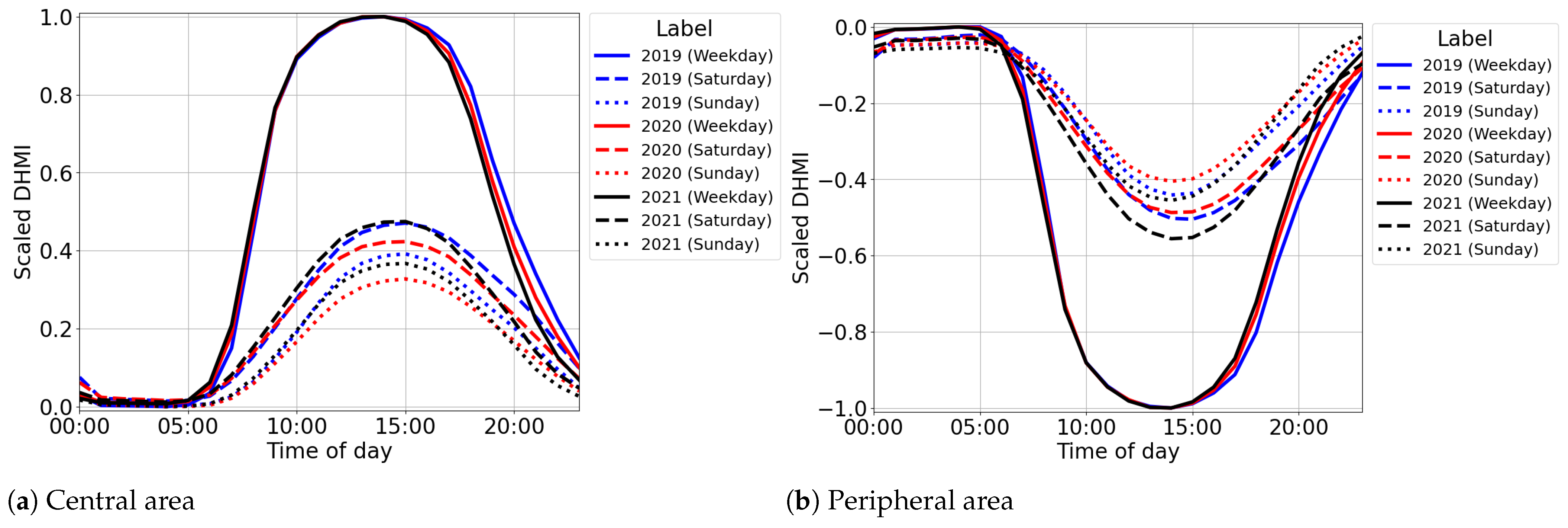
3.3.2. Diurnal Mobility Profile

The diurnal population profiles we found are shown in Figure 17. Based on the 36-month average diurnal profiles for the central area, the inflow of people began from 07:00 to 09:00, while the outflow began from around 17:00 to 21:00 on weekdays. The opposite pattern was observed in the peripheral area. In the evening, the slope of mobility is relatively lower and more varied due to the staggered return times from the urban area. Some individuals head straight home, while others may choose to dine or socialize before returning. In contrast, the morning commute is typically concentrated before office or school hours begin. On weekends, the timings of peak DHMI are generally similar to those on weekdays but with reduced mobility magnitude. Throughout the analysis period, mobility levels were consistently lower on Sunday compared to Saturday. On Saturday, mobility levels were 45.7% and 51.3% of the weekday levels in central and peripheral areas, respectively. On Sunday, mobility levels were 36.5% and 43.5% of weekday levels in central and peripheral areas, respectively. As discussed in Section 3.1.2, the differences may be attributed to Saturday school classes, six-day workweeks [55], or general behavioral tendencies for people to prefer to be stationary on Sundays. In addition, the greater reduction and variability in the central area on both Saturdays and Sundays may also be indicative of populations travelling farther away from Tokyo, which largely fluctuates during the weekends.

The 36-month profiles were well-aligned during weekday mornings, indicating a consistent behavior of people commuting to work at similar times while the time of returning home in the evening exhibited more variability, similar to the finding of [55]. In contrast, diurnal profiles on weekends showed greater variations in relative magnitude, departure times, and return times. In accordance with the findings of [63], this may imply that the daily travel activities during the weekends are less concentrated in the morning, as weekend trips are generally associated with activities that have fewer time constraints. Other factors that could potentially contribute to the variations include outlier “extreme” events and the seasons, which can easily influence weekend mobility. During the lockdown, the diurnal profiles significantly deviated from the 36-month averages, as depicted in Figure 18. The time people returned home was the fastest for both weekdays and weekends. Compared to weekdays, the mobility magnitudes during Saturdays and Sundays were remarkably reduced in the central and peripheral areas. In relation to weekdays, the mobility levels in the central area dropped to 25.9% (15.4%) for the Saturdays (Sundays) of April 2020, and to 36.1% (23.7%) for the Saturdays (Sundays) of May 2020. Similarly, in the peripheral areas, mobilities dropped to 29.1% (20.5%) for the Saturdays (Sundays) of April 2020, and to 38.9% (29.4%) for the Saturdays (Sundays) of May 2020.

The annual average diurnal profiles are illustrated in Figure 19, which depict the changes over the three-year period. While changes are more evident in the weekday profiles, similar trends can be observed in the order profiles. After the peak COVID-19 period, citizens tended to leave their residences slightly earlier in the morning and return home significantly earlier in the evening by the year. This evening trend aligns with [23], while the morning trend contradicts their findings, as they reported that morning activity began later during the period of the post-COVID-19 pandemic.

4. Conclusions

This study utilized high-resolution MSS data to derive and investigate collective human mobility, its patterns, and its correlation with public infrastructures in the Greater Tokyo Area from 2019 to 2021. At a 500 m spatial resolution, human mobility was classified into five typical daytime patterns of varying intensities of inflow and outflow levels: allweek_inflow, weekday_inflow, weekend_inflow, high_outflow, and low_outflow. For inflow patterns, a key distinguishing characteristic was the distinct levels of diurnal mobility between weekdays and weekends, while outflow patterns were defined based on their magnitude and irregularities. Approximately 55% of the inhabited areas over Tokyo were found to have high daytime human outflows. This was followed by around 15% of locations manifesting high inflow mainly during the weekdays and 12% of the locations experiencing higher weekend daytime inflows than during the weekdays. Almost 10% experienced balanced daytime inflows throughout all days of the week. Lastly, approximately 7% generally experienced daytime outflows but of relatively lower intensities.

To understand how these mobility patterns interact with urban spaces, the Chi-square test was performed for the relations between ten types of public infrastructures and derived mobility patterns. Certain infrastructures, such as police stations and hospitals, were found in locations of high daytime inflows. Here, both cities were presumed to be strategically located to ensure safety and at highly accessible locations, a characteristic of high daytime locations in the central areas. Meanwhile, other infrastructures, such as municipal offices and universities, possibly dictate mobility patterns, as indicated by their higher connection to certain mobility patterns, such as those of weekday_inflow and allweek_inflow. The analyses, however, did not find clear relations for a few public facilities, such as elderly welfare facilities and fire departments.

Additionally, human mobility over central and peripheral areas or at the intraregional level was estimated from the derived patterns. Prior to COVID-19, approximately 3 million people moved across these two areas daily. The diurnal mobility profiles showed a significant inflow of people into the central area during the daytime with the outflow towards the peripheral areas during the night. Variations in these profiles were also confirmed and could be observed during the weekends and the evening of weekdays. However, the restrictive effects of the COVID-19 lockdown on large-scale human mobility were apparent in both the magnitude and patterns of human mobility. Net human mobility decreased by 63% compared to pre-lockdown levels and the spatial distribution of the patterns underwent substantial changes during the lockdown period. Even after the lockdown was lifted, the reduced net mobility magnitude only recovered to approximately 70% of its original value. On the other hand, mobility patterns mostly returned to their original state with reduced spatial extent. During the lockdown, people tended to avoid coming home late on the weekdays and going out during the weekends.

It is important to note the limitations of this work. First, only Japanese and foreign residents are considered in the MSS data. The interpretations, therefore, do not extend to foreign tourists who visited Japan during the study period. As tourism in Japan has recovered over the past few years, understanding tourist mobility has become a promising topic for future research. Moreover, the detailed reasoning behind the characteristics and variations of human mobility patterns and diurnal profiles also requires further investigation. This study has not yet considered other factors that could influence human mobility, such as seasonality and climate parameters, but these can be further explored using the approach introduced in this work. This work mainly looked into COVID-19, which is a timely subject and which strongly affected mobilities during the defined period of the MSS dataset. Other factors, such as weather, may be examined by pairing the human mobility patterns with historical observations of weather (e.g., temperature, precipitation) in the studied location. A more comprehensive investigation into the influence of other factors on human mobility is left for future applications, particularly in the periods before and after COVID-19.

The conclusions from this investigation may provide a foundational or supporting basis for other areas, such as urban planning, risk reduction, and disaster resilience. By deeply understanding the characteristics of human mobility through the detection of human mobility patterns across diverse locations, appropriate site-specific policies may be formulated to accommodate various aspects or address societal issues. Urban-centered policies that may benefit from this work could be related to transportation systems management, urban planning, economic forecasting, public health, and environmental management [3,64]. Specifically, the methodology and findings introduced in this study may help identify congested areas over specific locations and periods within the region. This allows for better management of transportation systems and public spaces to be able to meet traffic and space demands. In the context of urban planning, the designation of new or relocation of old public facilities may also be aided by this work. In terms of the spread of diseases, the impacts of endemic spread and its responses examined in this and other similar studies indicate behavioral changes not only during the pandemic but also after the pandemic [23,30,61,62]. Similarly, spatial classification of human mobility is useful in drafting climate change mitigation and adaptation strategies, as well as in urban climate modeling. For example, human mobility maps may identify vulnerable locations and, hence, may help in the implementation of countermeasures in relevant areas [65]. In weather forecasting, these patterns may serve as inputs when constructing anthropogenic heat emission maps [66], representing an important weather model input that can influence the climate in cities and their surroundings.

References

1. Hannah, R.; Samborska, V.; Roser, M. Urbanization. 2024. Available online: https://ourworldindata.org/urbanization (accessed on 16 June 2024).
2. Lobo, J.; Aggarwal, R.M.; Alberti, M.; Allen-Dumas, M.; Bettencourt, L.M.; Boone, C.; Brelsford, C.; Broto, V.C.; Eakin, H.; Bagchi-Sen, S.; et al. Integration of Urban Science and Urban Climate Adaptation Research: Opportunities to Advance Climate Action. NPJ Urban Sustain. 2023, 3, 32. [Google Scholar] [CrossRef]
3. Wang, A.; Zhang, A.; Chan, E.H.W.; Shi, W.; Zhou, X.; Liu, Z. A Review of Human Mobility Research Based on Big Data and Its Implication for Smart City Development. ISPRS Int. J. Geo-Inf. 2021, 10, 13. [Google Scholar] [CrossRef]
4. Chen, Y.; Zhang, Z.; Lang, L.; Long, Z.; Wang, N.; Chen, X.; Wang, B.; Li, Y. Measuring the Spatial Match between Service Facilities and Population Distribution: Case of Lanzhou. Land 2023, 12, 1549. [Google Scholar] [CrossRef]
5. Wang, R.; Zhang, X.; Li, N. Zooming into mobility to understand cities: A review of mobility-driven urban studies. Cities 2022, 130, 103939. [Google Scholar] [CrossRef]
6. Bettencourt, L.M. The origins of scaling in cities. Science 2013, 340, 1438–1441. [Google Scholar] [CrossRef] [PubMed]
7. Wang, D.; Pedreschi, D.; Song, C.; Giannotti, F.; Barabasi, A.L. Human mobility, social ties, and link prediction. In Proceedings of the 17th ACM SIGKDD International Conference on Knowledge Discovery and Data Mining, San Diego, CA, USA, 21–24 August 2011; KDD ’11. pp. 1100–1108. [Google Scholar] [CrossRef]
8. Yabe, T.; Tsubouchi, K.; Fujiwara, N.; Wada, T.; Sekimoto, Y.; Ukkusuri, S.V. Non-compulsory measures sufficiently reduced human mobility in Tokyo during the COVID-19 epidemic. Sci. Rep. 2020, 10, 18053. [Google Scholar] [CrossRef] [PubMed]
9. Xiaomeng, C.; Guozhen, L.; Yang, Y.; Qingquan, L. Estimating the Distribution of Economy Activity: A Case Study in Jiangsu Province (China) Using Large Scale Social Network Data. In Proceedings of the 2014 IEEE International Conference on Data Mining Workshop, Shenzhen, China, 14 December 2014; pp. 1126–1134. [Google Scholar] [CrossRef]
10. Simini, F.; González, M.C.; Maritan, A.; Barabási, A.L. A universal model for mobility and migration patterns. Nature 2012, 484, 96–100. [Google Scholar] [CrossRef] [PubMed]
11. Wang, P.; González, M.C.; Hidalgo, C.A.; Barabási, A.L. Understanding Road Usage Patterns in Urban Areas. Sci. Rep. 2012, 2, 1001. [Google Scholar] [CrossRef]
12. Kraemer, M.U.G.; Golding, N.; Bisanzio, D.; Bhatt, S.; Pigott, D.M.; Ray, S.E.; Brady, O.J.; Brownstein, J.S.; Faria, N.R.; Cummings, D.A.T.; et al. Utilizing general human movement models to predict the spread of emerging infectious diseases in resource poor settings. Sci. Rep. 2019, 9, 5151. [Google Scholar] [CrossRef]
13. Tizzoni, M.; Bajardi, P.; Decuyper, A.; Kon Kam King, G.; Schneider, C.M.; Blondel, V.; Smoreda, Z.; González, M.C.; Colizza, V. On the use of human mobility proxies for modeling epidemics. PLoS Comput. Biol. 2014, 10, e1003716. [Google Scholar] [CrossRef]
14. Bengtsson, L.; Lu, X.; Thorson, A.; Garfield, R.; von Schreeb, J. Improved Response to Disasters and Outbreaks by Tracking Population Movements with Mobile Phone Network Data: A Post-Earthquake Geospatial Study in Haiti. PLOS Med. 2011, 8, e1001083. [Google Scholar] [CrossRef] [PubMed]
15. Barbosa, H.; Barthelemy, M.; Ghoshal, G.; James, C.R.; Lenormand, M.; Louail, T.; Menezes, R.; Ramasco, J.J.; Simini, F.; Tomasini, M. Human mobility: Models and applications. Phys. Rep. 2018, 734, 1–74. [Google Scholar] [CrossRef]
16. Brockmann, D.; Hufnagel, L.; Geisel, T. The scaling laws of human travel. Nature 2006, 439, 462–465. [Google Scholar] [CrossRef]
17. Song, C.; Koren, T.; Wang, P.; Barabási, A.L. Modelling the scaling properties of human mobility. Nat. Phys. 2010, 6, 818–823. [Google Scholar] [CrossRef]
18. Zipf, G.K. The P1 P2/D Hypothesis: On the Intercity Movement of Persons. Am. Sociol. Rev. 1946, 11, 677–686. [Google Scholar] [CrossRef]
19. Schläpfer, M.; Dong, L.; O’Keeffe, K.; Santi, P.; Szell, M.; Salat, H.; Anklesaria, S.; Vazifeh, M.; Ratti, C.; West, G.B. The Universal Visitation Law of Human mobility. Nature 2021, 593, 522–527. [Google Scholar] [CrossRef]
20. Chang, S.; Pierson, E.; Koh, P.W.; Gerardin, J.; Redbird, B.; Grusky, D.; Leskovec, J. Mobility network models of COVID-19 explain inequities and inform reopening. Nature 2021, 589, 82–87. [Google Scholar] [CrossRef]
21. Guo, P.; Sun, Y.; Chen, Q.; Li, J.; Liu, Z. The Impact of Rainfall on Urban Human Mobility from Taxi GPS Data. Sustainability 2022, 14, 9355. [Google Scholar] [CrossRef]
22. Schneider, C.M.; Belik, V.; Couronné, T.; Smoreda, Z.; González, M.C. Unraveling daily human mobility motifs. J. R. Soc. Interface 2013, 10, 20130246. [Google Scholar] [CrossRef]
23. Sparks, K.; Moehl, J.; Weber, E.; Brelsford, C.; Rose, A. Shifting temporal dynamics of human mobility in the United States. J. Transp. Geogr. 2022, 99, 103295. [Google Scholar] [CrossRef]
24. González, M.C.; Hidalgo, C.A.; Barabási, A.L. Understanding individual human mobility patterns. Nature 2008, 453, 779–782. [Google Scholar] [CrossRef] [PubMed]
25. Pan, Y.; Darzi, A.; Kabiri, A.; Zhao, G.; Luo, W.; Xiong, C.; Zhang, L. Quantifying human mobility behaviour changes during the COVID-19 outbreak in the United States. Sci. Rep. 2020, 10, 20742. [Google Scholar] [CrossRef] [PubMed]
26. Santana, C.; Botta, F.; Barbosa, H.; González, M.C.; Simini, F. COVID-19 is linked to changes in the time–space dimension of human mobility. Nat. Hum. Behav. 2023, 7, 1729–1739. [Google Scholar] [CrossRef]
27. Sulis, P.; Manley, E. Exploring similarities and variations of human mobility patterns in the city of London. Int. Arch. Photogramm. Remote Sens. Spat. Inf. Sci. 2018, 42, 51–58. [Google Scholar] [CrossRef]
28. Güller, C.; Varol, C. Unveiling the daily rhythm of urban space: Exploring the influence of built environment on spatiotemporal mobility patterns. Appl. Geogr. 2024, 170, 103366. [Google Scholar] [CrossRef]
29. Dai, J.; Schmöcker, J.D.; Sun, W. Analyzing demand reduction and recovery of major rail stations in Japan during COVID-19 using mobile spatial statistics. Asian Transp. Stud. 2024, 10, 100120. [Google Scholar] [CrossRef]
30. Santiago-Iglesias, E.; Romanillos, G.; Sun, W.; Schmöcker, J.D.; Moya-Gómez, B.; García-Palomares, J.C. Light in the darkness: Urban nightlife, analyzing the impact and recovery of COVID-19 using mobile phone data. Cities 2024, 153, 105276. [Google Scholar] [CrossRef]
31. Statista. Largest Urban Agglomerations Worldwide in 2023, by Population. Available online: https://www.statista.com/statistics/912263/population-of-urban-agglomerations-worldwide/ (accessed on 3 February 2025).
32. United Nations Department of Economic and Social Affairs. World Urbanization Prospects 2018: Highlights; UN: New York, NY, USA, 2019. [Google Scholar]
33. Cao, Z.; Asakura, Y.; Tan, Z. Coordination between node, place, and ridership: Comparing three transit operators in Tokyo. Transp. Res. Part Transp. Environ. 2020, 87, 102518. [Google Scholar] [CrossRef]
34. Tokyo Metropolitan Government. One day in Tokyo. Available online: https://www.tdh.metro.tokyo.lg.jp/english/faq/living/style.html (accessed on 3 February 2025).
35. West, G. Scale: The Universal Laws of Life, Growth, and Death in Organisms, Cities, and Companies; Penguin Books: Westminster, MD, USA, 2018. [Google Scholar]
36. Yong, N.; Ni, S.; Shen, S.; Chen, P.; Ji, X. Uncovering stable and occasional human mobility patterns: A case study of the Beijing subway. Phys. Stat. Mech. Its Appl. 2018, 492, 28–38. [Google Scholar] [CrossRef]
37. Terada, M.; Nagata, T.; Kobayashi, M. Population estimation technology for mobile spatial statistics. NTT DOCOMO Tech. J. 2013, 14, 10–15. [Google Scholar]
38. Mas, E.; Koshimura, S. Feasibility of anomalous event detection based on Mobile Spatial Statistics: A study of six cases in Japan. Int. J. Disaster Risk Reduct. 2024, 110, 104625. [Google Scholar] [CrossRef]
39. Kubo, T.; Uryu, S.; Yamano, H.; Tsuge, T.; Yamakita, T.; Shirayama, Y. Mobile phone network data reveal nationwide economic value of coastal tourism under climate change. Tour. Manag. 2020, 77, 104010. [Google Scholar] [CrossRef]
40. Akatsuka, H.; Toyoda, M. Analysis of the relationship between urban dynamics and prevalence of remote work based on population data generated from cellular networks. Sci. Rep. 2023, 13, 20139. [Google Scholar] [CrossRef] [PubMed]
41. Mizuno, T.; Ohnishi, T.; Watanabe, T. Visualizing Social and Behavior Change due to the Outbreak of COVID-19 Using Mobile Phone Location Data. New Gener. Comput. 2021, 39, 453–468. [Google Scholar] [CrossRef] [PubMed]
42. Arimura, M.; Ha, T.V.; Okumura, K.; Asada, T. Changes in urban mobility in Sapporo city, Japan due to the Covid-19 emergency declarations. Transp. Res. Interdiscip. Perspect. 2020, 7, 100212. [Google Scholar] [CrossRef]
43. Yamaguchi, H.; Nakayama, S. Pattern analysis of Japanese long-distance travel change under the COVID-19 pandemic. Transp. Res. Part Policy Pract. 2023, 176, 103805. [Google Scholar] [CrossRef]
44. Dantsuji, T.; Sugishita, K.; Fukuda, D. Understanding changes in travel patterns during the COVID-19 outbreak in the three major metropolitan areas of Japan. Transp. Res. Part A Policy Pract. 2023, 175, 103762. [Google Scholar] [CrossRef]
45. Hara, Y.; Yamaguchi, H. Japanese travel behavior trends and change under COVID-19 state-of-emergency declaration: Nationwide observation by mobile phone location data. Transp. Res. Interdiscip. Perspect. 2021, 9, 100288. [Google Scholar] [CrossRef]
46. Jin, X.; Han, J. K-Means Clustering. In Encyclopedia of Machine Learning; Springer US: Boston, MA, USA, 2010; pp. 563–564. [Google Scholar] [CrossRef]
47. Tavenard, R.; Faouzi, J.; Vandewiele, G.; Divo, F.; Androz, G.; Holtz, C.; Payne, M.; Yurchak, R.; Rußwurm, M.; Kolar, K.; et al. Tslearn, A Machine Learning Toolkit for Time Series Data. J. Mach. Learn. Res. 2020, 21, 1–6. [Google Scholar]
48. Cao, W.; Dong, L.; Cheng, Y.; Wu, L.; Guo, Q.; Liu, Y. Constructing multi-level urban clusters based on population distributions and interactions. Comput. Environ. Urban Syst. 2023, 99, 101897. [Google Scholar] [CrossRef]
49. Gupta, L.; Molfese, D.; Tammana, R.; Simos, P. Nonlinear alignment and averaging for estimating the evoked potential. IEEE Trans. Biomed. Eng. 1996, 43, 348–356. [Google Scholar] [CrossRef] [PubMed]
50. Jordahl, K.; den Bossche, J.V.; Fleischmann, M.; McBride, J.; Wasserman, J.; Badaracco, A.G.; Gerard, J.; Snow, A.D.; Tratner, J.; Perry, M.; et al. geopandas/geopandas: v0.10.2, 2021. Available online: https://zenodo.org/records/5573592 (accessed on 13 February 2025).
51. McHugh, M.L. The chi-square test of Independence. Biochem. Medica 2013, 23, 143–149. [Google Scholar] [CrossRef] [PubMed]
52. Pedregosa, F.; Varoquaux, G.; Gramfort, A.; Michel, V.; Thirion, B.; Grisel, O.; Blondel, M.; Prettenhofer, P.; Weiss, R.; Dubourg, V.; et al. Scikit-learn: Machine Learning in Python. J. Mach. Learn. Res. 2011, 12, 2825–2830. [Google Scholar]
53. Statistics Bureau of Japan. About Regional Mesh Statistics. Available online: https://www.stat.go.jp/data/mesh/m_tuite.html (accessed on 3 February 2025).
54. MLIT. National Land Numerical Information. National Land Numerical Information Download Site. Available online: https://nlftp.mlit.go.jp/ksj/index.html (accessed on 16 June 2024).
55. Umezaki, M.; Ishimaru, H.; Ohtsuka, R. Daily time budgets of long-distance commuting workers in tokyo megalopolis. J. Biosoc. Sci. 1999, 31, 71–78. [Google Scholar] [CrossRef] [PubMed]
56. Ishibashi, S.; Taniguchi, M. Workstyle change effects on physical activity and health consciousness in Japan: Results from COVID-19 lifestyle activity survey. Transp. Res. Interdiscip. Perspect. 2022, 15, 100657. [Google Scholar] [CrossRef]
57. Sun, Y.; Luo, S. A Study on the Current Situation of Public Service Facilities’ Layout from the Perspective of 15-Minute Communities—Taking Chengdu of Sichuan Province as an Example. Land 2024, 13, 1110. [Google Scholar] [CrossRef]
58. Jia, Y.; Zheng, Z.; Zhang, Q.; Li, M.; Liu, X. Associations of Spatial Aggregation between Neighborhood Facilities and the Population of Age Groups Based on Points-of-Interest Data. Sustainability 2020, 12, 1692. [Google Scholar] [CrossRef]
59. Ha, T.V.; Asada, T.; Arimura, M. Changes in mobility amid the COVID-19 pandemic in Sapporo City, Japan: An investigation through the relationship between spatiotemporal population density and urban facilities. Transp. Res. Interdiscip. Perspect. 2023, 17, 100744. [Google Scholar] [CrossRef]
60. MHLW. Open Data on COVID-19. Available online: https://www.mhlw.go.jp/stf/covid-19/open-data.html (accessed on 3 February 2025).
61. Javad Koohsari, M.; Nakaya, T.; Shibata, A.; Ishii, K.; Oka, K. Working from Home After the COVID-19 Pandemic: Do Company Employees Sit More and Move Less? Sustainability 2021, 13, 939. [Google Scholar] [CrossRef]
62. Kawaguchi, D.; Kitao, S.; Nose, M. The impact of COVID-19 on Japanese firms: Mobility and resilience via remote work. Int. Tax Public Financ. 2022, 29, 1419–1449. [Google Scholar] [CrossRef]
63. Herder, E.; Siehndel, P. Daily and weekly patterns in human mobility. In Proceedings of the 20th Conference on User Modeling, Adaptation, and Personalization, Montreal, Canada, 16–20 July 2012; pp. 338–340. [Google Scholar]
64. Batty, M.; Axhausen, K.W.; Giannotti, F.; Pozdnoukhov, A.; Bazzani, A.; Wachowicz, M.; Ouzounis, G.; Portugali, Y. Smart cities of the future. Eur. Phys. J. Spec. Top. 2012, 214, 481–518. [Google Scholar] [CrossRef]
65. Yu, S.; Lei, K.L.; Li, D.; Kim, Y.J.; Nemoto, M.; Gatson, S.; Yokohari, M.; Brown, R. Plan integration for urban extreme heat: Evaluating the impacts of plans at multiple scales in Tokyo, Japan. Urban Clim. 2024, 55, 101888. [Google Scholar] [CrossRef]
66. Varquez, A.C.G.; Kiyomoto, S.; Khanh, D.N.; Kanda, M. Global 1-km present and future hourly anthropogenic heat flux. Sci. Data 2021, 8, 64. [Google Scholar] [CrossRef] [PubMed]
Figure 1. Research framework. Sect. Ref. 1, 2, and 3 refers to Section 2.1, Section 2.2, and Section 2.3, respectively.
Urbansci 09 00050 g001
Figure 2. Section 2.1 flowchart.
Urbansci 09 00050 g002
Figure 3. Hourly (a) population ( P o p ) and (b) DHMI in the district of Shibuya. Each line with unique color represents a grid within Shibuya over a 4-day period.
Urbansci 09 00050 g003
Figure 4. Comparison between (a) Original DHMI and (b) Scaled DHMI (DHMI*) for two example grids (mesh A and mesh B).
Urbansci 09 00050 g004
Figure 5. Section 2.2 flowchart. Sect. Ref. 4 refers to Section 3.1.2.
Urbansci 09 00050 g005
Figure 6. Section 2.3 flowchart.
Urbansci 09 00050 g006
Figure 7. Classification of mobility pattern into inflow and outflow during April 2019.
Urbansci 09 00050 g007
Figure 8. Tokyo’s central area (red) and its boundary.
Urbansci 09 00050 g008
Figure 9. Comparison of identified peripheral areas between (a) April 2019 and (b) April 2020.
Urbansci 09 00050 g009
Figure 10. Residential population estimation in Tokyo during April 2019.
Urbansci 09 00050 g010
Figure 11. Human mobility on 15 April 2019 at (a) 00:00, (b) 07:00, (c) 14:00, and (d) 21:00.
Urbansci 09 00050 g011
Figure 12. Typical human mobility patterns. Region highlighted in gray represent weekends.
Urbansci 09 00050 g012
Figure 13. Map of mobility pattern classification in Tokyo during April 2019.
Urbansci 09 00050 g013
Figure 14. Map of mobility pattern classification during COVID-19 lockdown period: (a) April 2020; (b) May 2020.
Urbansci 09 00050 g014
Figure 15. Spatial distribution of (a) police stations, (b) hospitals, (c) child welfare facilities, annd (d) municipal offices.
Urbansci 09 00050 g015
Figure 16. Net DHMI during 36-month period in (a) central area and (b) peripheral area and during 4-month period in (c) central area and (d) peripheral area. Left vertical axis corresponds to hourly net DHMI (blue lines). Right vertical axis corresponds to total daily cases reported in Tokyo (red lines). Highlighted periods correspond to periods of state-of-emergency implementations.
Urbansci 09 00050 g016
Figure 17. Diurnal DHMI profiles of (a) central area and (b) peripheral area.
Urbansci 09 00050 g017
Figure 18. Diurnal DHMI profiles of (a) central area and (b) peripheral area during April and May 2020.
Urbansci 09 00050 g018
Figure 19. Annual average of DHMI profiles of (a) central area and (b) peripheral area for 2019 (blue), 2020 (red), and 2021 (black).
Urbansci 09 00050 g019