Adaptive Neural Fault-Tolerant Control for Nonlinear Fractional-Order Systems with Positive Odd Rational Powers

Abstract

In this paper, the problem of adaptive neural fault-tolerant control (FTC) for the fractional-order nonlinear systems (FNSs) with positive odd rational powers (PORPs) is considered. By using the radial basis function neural networks (RBF NNs), the unknown nonlinear functions from the controlled system can be approximated. With the help of an adaptive control ideology, the unknown control rate of the actuator fault can be handled. In particular, the FNSs subject to high-order terms are studied for the first time. In addition, the designed controller can ensure the boundedness of all the signals of the closed-loop control system, and the tracking error can tend to a small neighborhood of zero in the end. Finally, the illustrative examples are shown to validate the effectiveness of the developed method.

1. Introduction

The concept of Leibniz’s derivatives yielded the fractional-order calculus. As a generalization of integer-order differentiation and integration operators, the fractional-order calculus can describe many plants and processes precisely, such as physics, engineering, and economics, as in [1,2,3,4,5]. In the meantime, fractional-order controllers have more design freedom and a robust ability by comparing with integer-order ones [6]. Due to its wide application, the scholars are more enthusiastic about the control research of fractional-order systems. In [7], the authors proposed the Mittag-Leffler stability theory and further extended the Lyapunov direct method via utilizing the fractional-order operators. Aguila-Camacho et al. developed a new lemma for the Caputo fractional derivatives that can offer a simpler choice of the Lyapunov candidate function to the reader [8]. Based on the aforementioned research, in the field of the FNS, various interesting results were reported. The authors studied a sliding mode control approach for a class of chaotic FNSs in [9]. In terms of state [10] and output [11] feedback FNSs, the scholars presented corresponding adaptive controllers via the indirect Lyapunov method in [12], respectively. For fractional-order multiagent systems, an adaptive consensus control scheme was considered in [13]. With regard to uncertain fractional-order interconnected systems with unknown control directions, the fuzzy adaptive control approach was designed in [14]. In addition to the above results, there have also been massive and preeminent results in FNS fields (see [15,16,17,18,19,20]).

The nonlinear systems with PORP are also named as high-order nonlinear systems (HNSs). Because HNSs have uncontrollable linearization around the origin [21], in the design process of the controller a certain obstacle exists. Lin et al. presented a method called the adding a power integrator (API) which can deal with this difficulty effectively [22]. In addition, because of the strong approximation abilities of fuzzy logic systems (FLSs) and RBF NNs (such as [23,24,25,26]), the scholars used FLSs or RBF NNs as approximators to estimate the unknown nonlinearities compared to traditional control methods (such as [27,28,29]). Furthermore, a series of fruitful research was reported based on APIs and FLSs or RBF NNs. In terms of high-order multiagent nonlinear systems [30], the authors developed an adaptive output-feedback consensus tracking control scheme according to the state-observer method. For stochastic HNSs [31], Jiang et al. discussed the finite-time stabilization problem about high-order nonlinear systems with finite-time input-to-state stability inverse dynamics in 2019. In [32], although HNSs had input quantization, the adaptive neural tracking controller was still proposed. The authors considered fuzzy finite-time control theory for HNSs by the adaptive method in [33].

If actuator stoppage occurs in the practical situation, it may lead to performance deterioration and instability of the system, as described in [34]. For this reason, a lot of FTC schemes were designed and obtained numerous achievements. Tang et al. considered nonlinear multiple-input and multiple-output systems with an aircraft control application and designed an adaptive actuator failure compensation method in [35]. In [36], the authors studied the actuator failure compensation control of nonlinear systems with guaranteed transient performance in 2010. In terms of near-space vehicle attitude dynamics with actuator faults, Shen et al. investigated a fuzzy adaptive FTC issue in [37]. There are more interesting results on FTCs that are reported (see [38,39,40,41]). In addition, an FTC also yields a lot of results on an FNS. In [42], the fault-tolerant control methodology has been designed for FNSs. For the nonlinear interconnected FNS [43], Li et al. proposed an adaptive neural network scheme to deal with an FNS with intermittent actuator faults. In [44], the authors presented a series of fractional-order control approaches for a class of general nonlinear systems. The authors developed a new fractional-order adaptive control scheme based on a sliding mode configuration [45].

Despite the FTC mentioned earlier, there are problems that still need to be solved. Motivated by the above statements, in this paper, the adaptive tracking FTC problem for an FNS with PORP is considered. By combining RBF NNs and adaptive technology, an adaptive neural FTC controller is proposed, which can ensure all signals of the FNS with PORP are bounded, and the output signal can track the reference signal. The main contributions are outlined as follows:

(1) In this paper, the tracking control issue of the FNS with PORP is considered for the first time. In addition, the controlled system considers the condition of an actuator fault, which can be more suitable in practice.

(2) The proposed controller can not only guarantee that all signals of the FNS with PORP are bounded but also that the error of the FNS with PORP is near the origin. The ideology of the proposed control can also extend to a class of more general strict-feedback nonlinear systems.

The remaining part of the article can be outlined as follows. The preliminaries and problem formulation are given in Section 2. The design process of the proposed controller is introduced in Section 3. Section 4 provides the simulation results. The conclusions are drawn in Section 5.

2. Problem Formulation and Preliminaries

Consider the following FNS with PORP as follows:

$$\left\{\begin{array}{c}{D}^{\beta }{x}_i=x_{i+1}^{{\xi }_i}+f_i\left({\overline{x}}_i\right),i=1,2,\dots ,n-1\hfill \\ D^{\beta }{x}_n=u+f_n\left({\overline{x}}_n\right)\hfill \\ y=x_1,\hfill \end{array}\right.$$

where the fractional order $\beta \in (0,1)$, ${\overline{x}}_n={[x_1,\dots ,x_n]}^T\in R^n$ is the state vector with ${\overline{x}}_i={[x_1,\dots ,x_i]}^T\in R^i$ and $y\in R$ is output. $f_i(·)$, ($i=1,\dots ,n$) is unknown nonlinear function and u denotes the system input.

The system (1) is considered to occur the actuator fault:

$$\begin{array}{c}\hfill u^a\left(t\right)=\phi u+z\left(t\right)\end{array}$$

(1)

where $z\left(t\right)$ represents a bounded function and $0<{\phi }^{*}\le \phi \le 1$ indicates the remaining control rate and ${\phi }^{*}$ is a constant. When $u^a\left(t\right)=u+z\left(t\right)$, this indicates bias fault, and when $u^a\left(t\right)=\phi u$, this means gain fault. In addition, suppose that the actuator fault occurs at time instant $t_n$.

The control objective is to construct an adaptive FTC controller for FNS with PORP, such that:

(1)

All the signals in the FNS with PORP are proven to be bounded.

(2)

The tracking error can be able to tend to a small neighborhood near the origin.

Assumption 1

([46]). The sign of φ is known.

Assumption 2

([47]). The given reference signal $y_r$ is continuous and bounded; it also has nth order derivative.

Definition 1

([48]). There is a function $f:[t_0,+\infty )\to R$ that is abundant and smooth. Then, the Caputo fractional-order derivative with order β of f can be shown

$$\begin{array}{c}\hfill {}_c{D}_t^{\beta }f\left(t\right)=\frac{1}{\mathsf{{\rm Y}}(\mu -\beta )}{\int }_c^t\frac{f^{\left(\mu \right)}\left(\iota \right)}{{(t-\iota )}^{\beta -\mu +1}}d\iota \end{array}$$

(2)

where $\mu -1\le \beta <\mu$, $\mu \in N$. In addition, $\mathsf{{\rm Y}}\left(\beta \right)={\int }_0^{\infty }{y}^{\beta -1}{e}^{-y}dy$ is the Gamma function meeting $\mathsf{{\rm Y}}\left(1\right)=1$. When β is in $(0,1)$, $\mu =1$.

Remark 1.

In order for legibility, the fractional derivative of order β with the lower terminal at 0 is written as $D^{\beta }$ that can take the place of ${}_0{D}_t^{\beta }$.

According to the Laplace transform, (2) can be transformed as

$$\begin{array}{c}\hfill L\left\{D^{\beta }f\left(t\right)\right\}=s^{\beta }F\left(s\right)-\sum _{i=0}^{\mu -1}{s}^{\beta -i-1}{f}^{\left(i\right)}\left(0\right)\\ \hfill =s^{\beta }F\left(s\right)-s^{\beta -1}f\left(0\right)\end{array}$$

(3)

where $F\left(s\right)$ denotes the Laplace transform of $f\left(t\right)$. In our paper, $\beta \in (0,1)$ is only considered.

Definition 2

([48]). The Mittag-Leffler function with two parameters can be shown

$$\begin{array}{c}\hfill E_{\varrho ,b}=\sum _{i=0}^{\infty }\frac{{\varphi }^i}{\mathsf{{\rm Y}}(i\varrho +b)}\end{array}$$

(4)

where ϱ and b denote positive parameters, ϕ represents a complex number, and $E_{1,1}\left(\varphi \right)=e^{\varphi }$.

Based on the Laplace transform, (4) can be shown below

$$\begin{array}{c}\hfill L\left\{t^{b-1}{E}_{\varrho ,b}(-c{t}^{\varrho })\right\}=\frac{s^{\varrho -b}}{s^{\varrho }+c},(r\left(s\right){>\left|c\right|}^{-\varrho })\end{array}$$

(5)

where c is a real number and $r\left(s\right)$ is the real part of s.

The following two lemmas are proper for Mittag-Leffler function (4) and can be revealed as below:

Lemma 1

([48]). For all the number $\overline{\beta }\in R$ and the given number $q\in R$, there exists a real number ϱ ($\varrho \in (0,2)$), such that (6) holds with $\theta >0$ and $q\le |arg(\varphi \left)\right|\le \pi$.

$$\begin{array}{c}\hfill E_{\varrho ,\overline{\beta }}\le \frac{\theta }{1+\left|\varphi \right|}\end{array}$$

(6)

Lemma 2

([7]). Think about the FNS: $D^{\beta }y\left(t\right)=l(t,y\left(t\right))$, $l(·)$ meets Lipschitz condition and $y=0$ is an equilibrium point. Suppose some class—K functions $g_m(\parallel y\left(t\right)\parallel )(m=1,2,3)$ and $V(t,y(t\left)\right)$, which meet $g_1(\parallel y\left(t\right)\parallel )\le V\le g_2(\parallel y\left(t\right)\parallel )$ and $D^{\beta }V\le g_3(\parallel y\left(t\right)\parallel )$, then $D^{\beta }y\left(t\right)=l(t,y\left(t\right))$ is convergent and eventually stable, where $V(t,y(t\left)\right)$ is a function and $\beta \in (0,1)$.

Lemma 3

([8]). Let $g\left(t\right)\in R^n$ be a differentiable vector. For any time instant t

$$\begin{array}{c}\hfill \frac{1}{2}{D}^{\beta }\left(g^T\left(t\right)Pg\left(t\right)\right)\le g^T\left(t\right)P{D}^{\beta }g\left(t\right),\forall \beta \in (0,1],t\ge 0\end{array}$$

(7)

where $P\in R^{n\times n}$ is a positive definite constant matrix.

Lemma 4

([49]). It is supposed that the differentiable function $V\left(t\right)$ satisfying $V\left(0\right)$ is non-negative. If $V\left(t\right)$ can satisfy $D^{\beta }V\left(t\right)\le -\chi V\left(t\right)+d_o$, $V\left(t\right)\le \varsigma (V\left(0\right)+\frac{d_o}{\chi })$, where $\chi >0$, $\varsigma >0$ and $d_o>0$ are parameters.

Lemma 5

([50]). With regard to any real-valued function $\nu ,\zeta$ and any positive odd integer $\xi \ge 1$, then $\left|{\nu }^{\xi }-{\zeta }^{\xi }\right|\le \xi \left|\nu -\zeta \right|({\nu }^{\xi -1}+{\zeta }^{\xi -1})$.

The RBF NN is utilized to shape the unknown nonlinear function $f\left(P\right):R^q\to R$, which is described as

$$f_{nn}\left(P\right)=W^T\Psi \left(P\right)$$

(8)

where $P\in {\mathsf{\Omega }}_P\subset R^q$ denotes the input vector and $W={[w_1,\dots ,w_{\overline{l}}]}^T\in R^{\overline{l}}$ represents weight vector with the RBF NN node number $\overline{l}>1$. $\Psi \left(P\right)={[s_1\left(P\right),\dots ,s_{\overline{l}}\left(P\right)]}^T\in R^{\overline{l}}$. $s_i\left(P\right)$ is chosen as commonly used Gaussian function:

$$s_i\left(P\right)=e^{-\frac{{(P-v_i)}^T(P-v_i)}{{\eta }_i^2}},1\le i\le \overline{l}$$

(9)

where the center of the receptive domain is denoted by $v_i={[v_{i1},\dots ,v_{iq}]}^T$ and ${\eta }_i$ represents the width of the Gaussian function.

From [51], if $\overline{l}$ is selected sufficiently large, $W^T\Psi \left(Y\right)$ can approximate any continuous function $f\left(P\right)$ to any desired accuracy over a compact set ${\mathsf{\Omega }}_P\subset R^q$ to arbitrary accuracy in

$$f\left(P\right)=W^{*T}\Psi \left(P\right)+\kappa \left(P\right),\forall P\in {\mathsf{\Omega }}_P\subset R^q$$

(10)

The $W^{*}$ in (10) is the optimal weight vector that can be shown as

$$W^{*}=arg\underset{W\in R^l}{min}\{\underset{P\in {\mathsf{\Omega }}_P}{sup}|f\left(P\right)-W^T\Psi \left(P\right)\left|\right\}$$

(11)

where the approximation error can be shown as $\kappa \left(P\right)$ and it can satisfy $\kappa \left(P\right)<\varpi$ for any given constant $\varpi >0$.

3. Design of Controller

The coordinate transformations are given below

$$\left\{\begin{array}{c}{\alpha }_1=x_1-y_r,\hfill \\ {\alpha }_i=x_i-{\lambda }_{i-1},i=2,\dots ,n\hfill \end{array}\right.$$

where ${\lambda }_i$ is the virtual control law.

Step 1. It is easy to obtain

$$\begin{array}{c}\hfill D^{\beta }{\alpha }_1=D^{\beta }{x}_1-D^{\beta }{y}_r=x_2^{{\xi }_1}+f_1\left({\overline{x}}_1\right)-D^{\beta }{y}_r\end{array}$$

(12)

A Lyapunov function can be defined as follows

$$V_1=\frac{1}{2}{\alpha }_1^2+\frac{1}{2{\rho }_1}{\tilde{\sigma }}_1^2$$

(13)

where ${\tilde{\sigma }}_1={\sigma }_1-{\widehat{\sigma }}_1$, ${\rho }_1$ is a positive constant. With the help of Lemma 3, then

$$\begin{array}{c}\hfill D^{\beta }{V}_1\le {\alpha }_1{D}^{\beta }{\alpha }_1-\frac{1}{{\rho }_1}{\tilde{\sigma }}_1{D}^{\beta }{\widehat{\sigma }}_1\\ \hfill ={\alpha }_1(x_2^{{\xi }_1}+f_1\left({\overline{x}}_1\right)-D^{\beta }{y}_r)-\frac{1}{{\rho }_1}{\tilde{\sigma }}_1{D}^{\beta }{\widehat{\sigma }}_1\\ \hfill ={\alpha }_1(x_2^{{\xi }_1}-{\lambda }_1^{{\xi }_1}+{\lambda }_1^{{\xi }_1}+f_1\left({\overline{x}}_1\right)-D^{\beta }{y}_r)-\frac{1}{{\rho }_1}{\tilde{\sigma }}_1{D}^{\beta }{\widehat{\sigma }}_1\end{array}$$

(14)

Let us define ${\overline{f}}_1\left({\overline{x}}_1\right)=f_1\left({\overline{x}}_1\right)-D^{\beta }{y}_r+\frac{{\alpha }_1}{2}+\frac{{\xi }_1^2{\alpha }_1}{2}$. Due to the existence of unknown nonlinear function $f_1\left({\overline{x}}_1\right)$, we can use RBF NNs to approximate ${\overline{f}}_1\left({\overline{x}}_1\right)$, one has ${\overline{f}}_1\left({\overline{x}}_1\right)=W_1^T{\Psi }_1\left({\overline{x}}_1\right)+{\kappa }_1,\left|{\kappa }_1\right|\le {\varpi }_1$ and ${\varpi }_1$ is a constant.

Based on Young’s inequality, we can obtain

$$\begin{array}{c}\hfill {\alpha }_1{\overline{f}}_1\left({\overline{x}}_1\right)\le \frac{1}{2b_1^2}{\alpha }_1^2{\sigma }_1{\Psi }_1^T{\Psi }_1+\frac{b_1^2}{2}+\frac{{\alpha }_1^2}{2}+\frac{{\varpi }_1^2}{2}\end{array}$$

(15)

where ${\sigma }_1={\parallel W_1\parallel }^2$, $b_1>0$ is a design constant.

Then, we can rewrite $D^{\beta }{V}_1$ as

$$\begin{array}{c}\hfill D^{\beta }{V}_1\le {\alpha }_1(x_2^{{\xi }_1}-{\lambda }_1^{{\xi }_1}+{\lambda }_1^{{\xi }_1}+\frac{1}{2b_1^2}{\alpha }_1{\sigma }_1{\Psi }_1^T{\Psi }_1)\\ \hfill -\frac{1}{{\rho }_1}{\tilde{\sigma }}_1{D}^{\beta }{\widehat{\sigma }}_1+\frac{b_1^2}{2}+\frac{{\varpi }_1^2}{2}-\frac{{\xi }_1^2{\alpha }_1^2}{2}\end{array}$$

(16)

In addition, with the help of Lemma 5, then

$$\begin{array}{c}\hfill {\alpha }_1(x_2^{{\xi }_1}-{\lambda }_1^{{\xi }_1})\le {\xi }_1|{\alpha }_1\left|\right|{\alpha }_2|(x_2^{{\xi }_1-1}+{\lambda }_1^{{\xi }_1-1})\\ \hfill \le \frac{{\xi }_1^2{\alpha }_1^2}{2}+\frac{1}{2}{\alpha }_2^2{(x_2^{{\xi }_1-1}+{\lambda }_1^{{\xi }_1-1})}^2\end{array}$$

(17)

From (17), $D^{\beta }{V}_1$ can be written as

$$\begin{array}{c}\hfill D^{\beta }{V}_1\le {\alpha }_1({\lambda }_1^{{\xi }_1}+\frac{1}{2b_1^2}{\alpha }_1{\widehat{\sigma }}_1{\Psi }_1^T{\Psi }_1)\\ \hfill +\frac{1}{{\rho }_1}{\tilde{\sigma }}_1(\frac{{\rho }_1}{2b_1^2}{\alpha }_1^2{\Psi }_1^T{\Psi }_1-D^{\beta }{\widehat{\sigma }}_1)\\ \hfill +\frac{b_1^2}{2}+\frac{{\varpi }_1^2}{2}+\frac{1}{2}{\alpha }_2^2{(x_2^{{\xi }_1-1}+{\lambda }_1^{{\xi }_1-1})}^2\end{array}$$

(18)

We design the virtual control law ${\lambda }_1$ and the adaptive law $D^{\beta }{\widehat{\sigma }}_1$ as follows

$$\begin{array}{c}\hfill {\lambda }_1=-{(c_1{\alpha }_1+\frac{1}{2b_1^2}{\alpha }_1{\widehat{\sigma }}_1{\Psi }_1^T{\Psi }_1)}^{\frac{1}{{\xi }_1}},\\ \hfill D^{\beta }{\widehat{\sigma }}_1=\frac{{\rho }_1}{2b_1^2}{\alpha }_1^2{\Psi }_1^T{\Psi }_1-o_1{\widehat{\sigma }}_1\end{array}$$

(19)

where $c_1$ is a positive design constant.

Furthermore, inequality (18) can be written as

$$\begin{array}{c}\hfill D^{\beta }{V}_1\le -c_1{\alpha }_1^2+\frac{b_1^2}{2}+\frac{{\varpi }_1^2}{2}+\frac{o_1}{{\rho }_1}{\tilde{\sigma }}_1{\widehat{\sigma }}_1\\ \hfill +\frac{1}{2}{\alpha }_2^2{(x_2^{{\xi }_1-1}+{\lambda }_1^{{\xi }_1-1})}^2\end{array}$$

(20)

Step 2. $D^{\beta }{\alpha }_2$ can be shown as

$$\begin{array}{c}\hfill D^{\beta }{\alpha }_2=D^{\beta }{x}_2-D^{\beta }{\lambda }_1=x_3^{{\xi }_2}+f_2\left({\overline{x}}_2\right)-D^{\beta }{\lambda }_1\end{array}$$

(21)

The designed Lyapunov function as

$$V_2=\frac{1}{2}{\alpha }_2^2+\frac{1}{2{\rho }_2}{\tilde{\sigma }}_2^2+V_1$$

(22)

where ${\tilde{\sigma }}_2={\sigma }_2-{\widehat{\sigma }}_2$, ${\rho }_2>0$ is a constant.

Similar to (14), then

$$\begin{array}{c}\hfill D^{\beta }{V}_2\le {\alpha }_2{D}^{\beta }{\alpha }_2-\frac{1}{{\rho }_2}{\tilde{\sigma }}_2{D}^{\beta }{\widehat{\sigma }}_2+D^{\beta }{V}_1\\ \hfill ={\alpha }_2(x_3^{{\xi }_2}+f_2\left({\overline{x}}_2\right)-D^{\beta }{\lambda }_1+\frac{1}{2}{\alpha }_2{(x_2^{{\xi }_1-1}+{\lambda }_1^{{\xi }_1-1})}^2)\\ \hfill -\frac{1}{{\rho }_2}{\tilde{\sigma }}_2{D}^{\beta }{\widehat{\sigma }}_2-c_1{\alpha }_1^2+\frac{b_1^2}{2}+\frac{{\varpi }_1^2}{2}+\frac{o_1}{{\rho }_1}{\tilde{\sigma }}_1{\widehat{\sigma }}_1\\ \hfill ={\alpha }_2(x_3^{{\xi }_2}-{\lambda }_2^{{\xi }_2}+{\lambda }_2^{{\xi }_2}+{\overline{f}}_2\left({\overline{x}}_2\right))\\ \hfill -\frac{{\alpha }_2^2}{2}-\frac{{\xi }_2^2{\alpha }_2^2}{2}-\frac{1}{{\rho }_2}{\tilde{\sigma }}_2{D}^{\beta }{\widehat{\sigma }}_2-c_1{\alpha }_1^2+\frac{b_1^2}{2}\\ \hfill +\frac{{\varpi }_1^2}{2}+\frac{o_1}{{\rho }_1}{\tilde{\sigma }}_1{\widehat{\sigma }}_1\end{array}$$

(23)

Let us define ${\overline{f}}_2\left({\overline{x}}_2\right)=f_2\left({\overline{x}}_2\right)-D^{\beta }{\lambda }_1+\frac{{\alpha }_2}{2}+\frac{{\xi }_2^2{\alpha }_2}{2}+1/2{\alpha }_2{(x_2^{{\xi }_1-1}+{\lambda }_1^{{\xi }_1-1})}^2$. By using RBF NNs to approximate ${\overline{f}}_2\left({\overline{x}}_2\right)$, then ${\overline{f}}_2\left({\overline{x}}_2\right)=W_2^T{\Psi }_2\left({\overline{x}}_2\right)+{\kappa }_2,\left|{\kappa }_2\right|\le {\varpi }_2$ and ${\varpi }_2$ is a constant. With the support of Young’s inequality, then

$$\begin{array}{c}\hfill {\alpha }_2{\overline{f}}_2\left({\overline{x}}_2\right)\le \frac{1}{2b_2^2}{\alpha }_2^2{\sigma }_2{\Psi }_2^T{\Psi }_2+\frac{b_2^2}{2}+\frac{{\alpha }_2^2}{2}+\frac{{\varpi }_2^2}{2}\end{array}$$

(24)

where ${\sigma }_2={\parallel W_2\parallel }^2$, $b_2>0$ is a design constant.

The same as (17), with the help of Lemma 5, then

$$\begin{array}{c}\hfill {\alpha }_2(x_3^{{\xi }_2}-{\lambda }_2^{{\xi }_2})\le {\xi }_2|{\alpha }_2\left|\right|{\alpha }_3|(x_3^{{\xi }_2}+{\lambda }_2^{{\xi }_2})\\ \hfill \le \frac{{\xi }_2^2{\alpha }_2^2}{2}+\frac{1}{2}{\alpha }_3^2{(x_3^{{\xi }_2-1}+{\lambda }_2^{{\xi }_2-1})}^2\end{array}$$

(25)

Next, the virtual control law ${\lambda }_2$ and the adaptive law $D^{\beta }{\widehat{\sigma }}_2$ can be designed

$$\begin{array}{c}\hfill {\lambda }_2=-{(c_2{\alpha }_2+\frac{1}{2b_2^2}{\alpha }_2{\widehat{\sigma }}_2{\Psi }_2^T{\Psi }_2)}^{\frac{1}{{\xi }_2}},\end{array}$$

(26)

$$\begin{array}{c}\hfill D^{\beta }{\widehat{\sigma }}_2=\frac{{\rho }_2}{2b_2^2}{\alpha }_2^2{\Psi }_2^T{\Psi }_2-o_2{\widehat{\sigma }}_2\end{array}$$

(27)

where $c_2>0$ is a design parameter.

By substituting (26) and (27) into (23), we can obtain

$$\begin{array}{c}\hfill D^{\beta }{V}_2\le -\sum _{h=1}^2{c}_h{\alpha }_h^2+\sum _{h=1}^2\frac{b_h^2}{2}+\sum _{h=1}^2\frac{{\varpi }_h^2}{2}\\ \hfill +\sum _{h=1}^2\frac{o_h}{{\rho }_h}{\tilde{\sigma }}_h{\widehat{\sigma }}_h+\frac{1}{2}{\alpha }_3^2{(x_3^{{\xi }_2-1}+{\lambda }_2^{{\xi }_2-1})}^2\end{array}$$

(28)

Stepi$(3\le i\le n-1)$. The Lyapunov function is designed as follows

$$V_i=\frac{1}{2}{\alpha }_i^2+\frac{1}{2{\rho }_i}{\tilde{\sigma }}_i^2+V_{i-1}$$

(29)

where ${\tilde{\sigma }}_i={\sigma }_i-{\widehat{\sigma }}_i$, ${\rho }_i>0$ is a constant.

It is obvious to obtain

$$\begin{array}{c}\hfill D^{\beta }{V}_i\le {\alpha }_i{D}^{\beta }{\alpha }_i-\frac{1}{{\rho }_i}{\tilde{\sigma }}_i{D}^{\beta }{\widehat{\sigma }}_i+D^{\beta }{V}_{i-1}\\ \hfill ={\alpha }_i(x_{i+1}^{{\xi }_i}+f_i\left({\overline{x}}_i\right)-D^{\beta }{\lambda }_{i-1})\\ \hfill -\frac{1}{{\rho }_i}{\tilde{\sigma }}_i{D}^{\beta }{\widehat{\sigma }}_i+D^{\beta }{V}_{i-1}\\ \hfill ={\alpha }_i(x_{i+1}^{{\xi }_i}-{\lambda }_i^{{\xi }_i}+{\lambda }_i^{{\xi }_i}+f_i\left({\overline{x}}_i\right)-D^{\beta }{\lambda }_{i-1})\\ \hfill -\frac{1}{{\rho }_i}{\tilde{\sigma }}_i{D}^{\beta }{\widehat{\sigma }}_i+D^{\beta }{V}_{i-1}\end{array}$$

(30)

Define ${\overline{f}}_i\left({\overline{x}}_i\right)=f_i\left({\overline{x}}_i\right)-D^{\beta }{\lambda }_{i-1}+\frac{{\alpha }_i}{2}+\frac{{\xi }_i^2{\alpha }_i}{2}+\frac{1}{2}{\alpha }_i{(x_i^{{\xi }_{i-1}-1}+{\lambda }_{i-1}^{{\xi }_{i-1}-1})}^2$. The same as step 1, by using RBF NNs to approximate ${\overline{f}}_i\left({\overline{x}}_i\right)$, then ${\overline{f}}_i\left({\overline{x}}_i\right)=W_i^T{\Psi }_i\left({\overline{x}}_i\right)+{\kappa }_i,\left|{\kappa }_i\right|\le {\varpi }_i$, where ${\varpi }_i$ is a constant. According to Young’s inequality, then

$$\begin{array}{c}\hfill {\alpha }_i{\overline{f}}_i\left({\overline{x}}_i\right)\le \frac{1}{2b_i^2}{\alpha }_i^2{\sigma }_i{\Psi }_i^T{\Psi }_i+\frac{b_i^2}{2}+\frac{{\alpha }_i^2}{2}+\frac{{\varpi }_i^2}{2}\end{array}$$

(31)

where ${\sigma }_i={\parallel W_i\parallel }^2$, $b_i>0$ is a design constant.

Next, we start to deal with ${\alpha }_i(x_{i+1}^{{\xi }_i}-{\lambda }_i^{{\xi }_i})$ with the support of Lemma 5, then

$$\begin{array}{c}\hfill {\alpha }_i(x_{i+1}^{{\xi }_i}-{\lambda }_i^{{\xi }_i})\le {\xi }_i|{\alpha }_i\left|\right|{\alpha }_{i+1}|(x_{i+1}^{{\xi }_i-1}+{\lambda }_i^{{\xi }_i-1})\\ \hfill \le \frac{{\xi }_i^2{\alpha }_i^2}{2}+\frac{1}{2}{\alpha }_{i+1}^2{(x_{i+1}^{{\xi }_i-1}+{\lambda }_i^{{\xi }_i-1})}^2\end{array}$$

(32)

On the basis of (31) and (32), we obtain

$$\begin{array}{c}\hfill D^{\beta }{V}_i\le {\alpha }_i({\lambda }_i^{{\xi }_i}+\frac{1}{2b_i^2}{\alpha }_i{\widehat{\sigma }}_i{\Psi }_i^T{\Psi }_i)\\ \hfill +\frac{1}{{\rho }_i}{\tilde{\sigma }}_i(\frac{{\rho }_i}{2b_i^2}{\alpha }_i^2{\Psi }_i^T{\Psi }_i-D^{\beta }{\widehat{\sigma }}_i)+D^{\beta }{V}_{i-1}\\ \hfill +\frac{b_i^2}{2}+\frac{{\varpi }_i^2}{2}+\frac{1}{2}{\alpha }_{i+1}^2{(x_{i+1}^{{\xi }_i-1}+{\lambda }_i^{{\xi }_i-1})}^2\end{array}$$

(33)

We can design the virtual control law ${\lambda }_i$ and the adaptive law $D^{\beta }{\widehat{\sigma }}_i$, one has

$$\begin{array}{c}\hfill {\lambda }_i=-{(c_i{\alpha }_i+\frac{1}{2b_i^2}{\alpha }_i{\widehat{\sigma }}_i{\Psi }_i^T{\Psi }_i)}^{\frac{1}{{\xi }_i}},\end{array}$$

(34)

$$\begin{array}{c}\hfill D^{\beta }{\widehat{\sigma }}_i=\frac{{\rho }_i}{2b_i^2}{\alpha }_i^2{\Psi }_i^T{\Psi }_i-o_i{\widehat{\sigma }}_i\end{array}$$

(35)

where $c_i>0$ is a design constant.

Substituting (34) and (35) into (33), we can obtain

$$\begin{array}{c}\hfill D^{\beta }{V}_i\le -\sum _{h=1}^i{c}_h{\alpha }_h^2+\sum _{h=1}^i\frac{b_h^2}{2}+\sum _{h=1}^i\frac{{\varpi }_h^2}{2}\\ \hfill +\sum _{h=1}^i\frac{o_h}{{\rho }_h}{\tilde{\sigma }}_h{\widehat{\sigma }}_h+\frac{1}{2}{\alpha }_{i+1}^2{(x_{i+1}^{{\xi }_i-1}+{\lambda }_i^{{\xi }_i-1})}^2\end{array}$$

(36)

Stepn. We ultimately design actual control law u and the adaptive laws $D^{\beta }{\widehat{\sigma }}_n$ and $D^{\beta }\widehat{v}$ in this position as

$$\left\{\begin{array}{c}u=\widehat{v}\overline{u},\hfill \\ \overline{u}=-c_n{\alpha }_n-\frac{1}{2b_n^2}{\alpha }_n{\widehat{\sigma }}_n{\Psi }_n^T{\Psi }_n-z\left(t\right),\hfill \\ D^{\beta }{\widehat{\sigma }}_n=\frac{{\rho }_n}{2b_n^2}{\alpha }_n^2{\Psi }_n^T{\Psi }_n-o_n{\widehat{\sigma }}_n,\hfill \\ D^{\beta }\widehat{v}=-\gamma sign\left(\phi \right)\overline{u}{\alpha }_n-o_c\widehat{v}\hfill \end{array}\right.$$

(37)

where $v=\frac{1}{\phi }$, $\tilde{v}=v-\widehat{v}$, ${\tilde{\sigma }}_n={\sigma }_n-{\widehat{\sigma }}_n$ and $\gamma >0$, ${\rho }_n>0$, $c_n>0$, $b_n>0$, $o_n>0$ and $o_c>0$ are constants. It is noted that $\phi u=\overline{u}-\phi \tilde{v}\overline{u}$.

Next, the following Lyapunov function candidate is chosen

$$V_n=\frac{1}{2}{\alpha }_n^2+\frac{1}{2{\rho }_n}{\tilde{\sigma }}_n^2+\frac{\left|\phi \right|}{2\gamma }{\tilde{v}}^2+V_{n-1}$$

(38)

Using Lemma 3, it is not difficult to obtain

$$\begin{array}{c}\hfill D^{\beta }{V}_n\le {\alpha }_n(\phi u+z\left(t\right)+f_n\left({\overline{x}}_n\right)-D^{\beta }{\lambda }_{n-1})\\ \hfill -\frac{1}{{\rho }_n}{\tilde{\sigma }}_n{D}^{\beta }{\widehat{\sigma }}_n+D^{\beta }{V}_{n-1}-\frac{\left|\phi \right|}{\gamma }\tilde{v}{D}^{\beta }\widehat{v}\end{array}$$

(39)

The same as the previous steps, we define ${\overline{f}}_n\left({\overline{x}}_n\right)=f_n\left({\overline{x}}_n\right)-D^{\beta }{\lambda }_{n-1}+\frac{{\alpha }_n}{2}+\frac{{\xi }_n^2{\alpha }_n}{2}+\frac{1}{2}{\alpha }_n{(x_n^{{\xi }_{n-1}-1}+{\lambda }_{n-1}^{{\xi }_{n-1}-1})}^2$. By employing RBF NNs to approximate ${\overline{f}}_n\left({\overline{x}}_n\right)$, then ${\overline{f}}_n\left({\overline{x}}_n\right)=W_n^T{\Psi }_n\left({\overline{x}}_n\right)+{\kappa }_n,\left|{\kappa }_n\right|\le {\varpi }_n$, where ${\varpi }_n$ is a constant. Next, we define that ${\sigma }_n={\parallel W_n\parallel }^2$ and utilize Young’s inequality, then

$$\begin{array}{c}\hfill {\alpha }_n{\overline{f}}_n\left({\overline{x}}_n\right)\le \frac{1}{2b_n^2}{\alpha }_n^2{\sigma }_n{\Psi }_n^T{\Psi }_n+\frac{b_n^2}{2}+\frac{{\alpha }_n^2}{2}+\frac{{\varpi }_n^2}{2}\end{array}$$

(40)

We can substitute (37) into (39), and one has

$$\begin{array}{c}\hfill D^{\beta }{V}_n\le {\alpha }_n(\overline{u}+z\left(t\right)+\frac{1}{2b_n^2}{\widehat{\sigma }}_n{\Psi }_n^T{\Psi }_n)\\ \hfill +\frac{{\tilde{\sigma }}_n}{{\rho }_n}(\frac{{\rho }_n}{2b_n^2}{\alpha }_n^2{\Psi }_n^T{\Psi }_n-D^{\beta }{\widehat{\sigma }}_n)+D^{\beta }{V}_{n-1}\\ \hfill -\frac{\left|\phi \right|}{\gamma }\tilde{v}(D^{\beta }\widehat{v}+\gamma sign\left(\phi \right)\overline{u}{\alpha }_n)\\ \hfill \le -\sum _{h=1}^n{c}_h{\alpha }_h^2+\sum _{h=1}^n\frac{o_h}{{\rho }_h}{\tilde{\sigma }}_h{\widehat{\sigma }}_h+\frac{\left|\phi \right|}{\gamma }\tilde{v}\widehat{v}\\ \hfill +\sum _{h=1}^n\frac{b_h^2}{2}+\sum _{h=1}^n\frac{{\varpi }_h^2}{2}\end{array}$$

(41)

Because the definitions of ${\tilde{\sigma }}_h$ ($h=1,\dots ,n$) and $\tilde{v}$, we can obtain the following inequalities:

$$\begin{array}{c}\hfill \sum _{h=1}^n\frac{o_h}{{\rho }_h}{\tilde{\sigma }}_h{\widehat{\sigma }}_h\le -\sum _{h=1}^n\frac{o_h}{2{\rho }_h}{\tilde{\sigma }}_h^2+\sum _{h=1}^n\frac{o_h}{2{\rho }_h}{\sigma }_h^2\end{array}$$

(42)

$$\begin{array}{c}\hfill \frac{\left|\phi \right|}{\gamma }\tilde{v}\widehat{v}\le -o_c\frac{\left|\phi \right|}{2\gamma }{\tilde{v}}^2+o_c\frac{\left|\phi \right|}{2\gamma }{v}^2\end{array}$$

(43)

From the above inequalities (42) and (43), we can derive the following inequality

$$\begin{array}{c}\hfill D^{\beta }{V}_n\le -\sum _{h=1}^n{c}_h{\alpha }_h^2-\sum _{h=1}^n\frac{o_h}{2{\rho }_h}{\tilde{\sigma }}_h^2-o_c\frac{\left|\phi \right|}{2\gamma }{\tilde{v}}^2+d_o\end{array}$$

(44)

where $d_o={\sum }_{h=1}^n\frac{b_h^2}{2}+{\sum }_{h=1}^n\frac{{\varpi }_h^2}{2}+{\sum }_{h=1}^n\frac{o_h}{2{\rho }_h}{\sigma }_h^2+o_c\frac{\left|\phi \right|}{2\gamma }{v}^2$.

Theorem 1.

Design the actual law u, the virtual control laws ${\lambda }_h$ ($h=1,2,\dots ,n-1$), and the adaptive laws $D^{\beta }{\widehat{\sigma }}_h$ ($h=1,2,\dots ,n$) and $D^{\beta }\widehat{v}$ for the FNS with PORP (1) with Assumption 1, then we have the following properties:

(1) 

All signals of the FNS with PORP are bounded.

(2) 

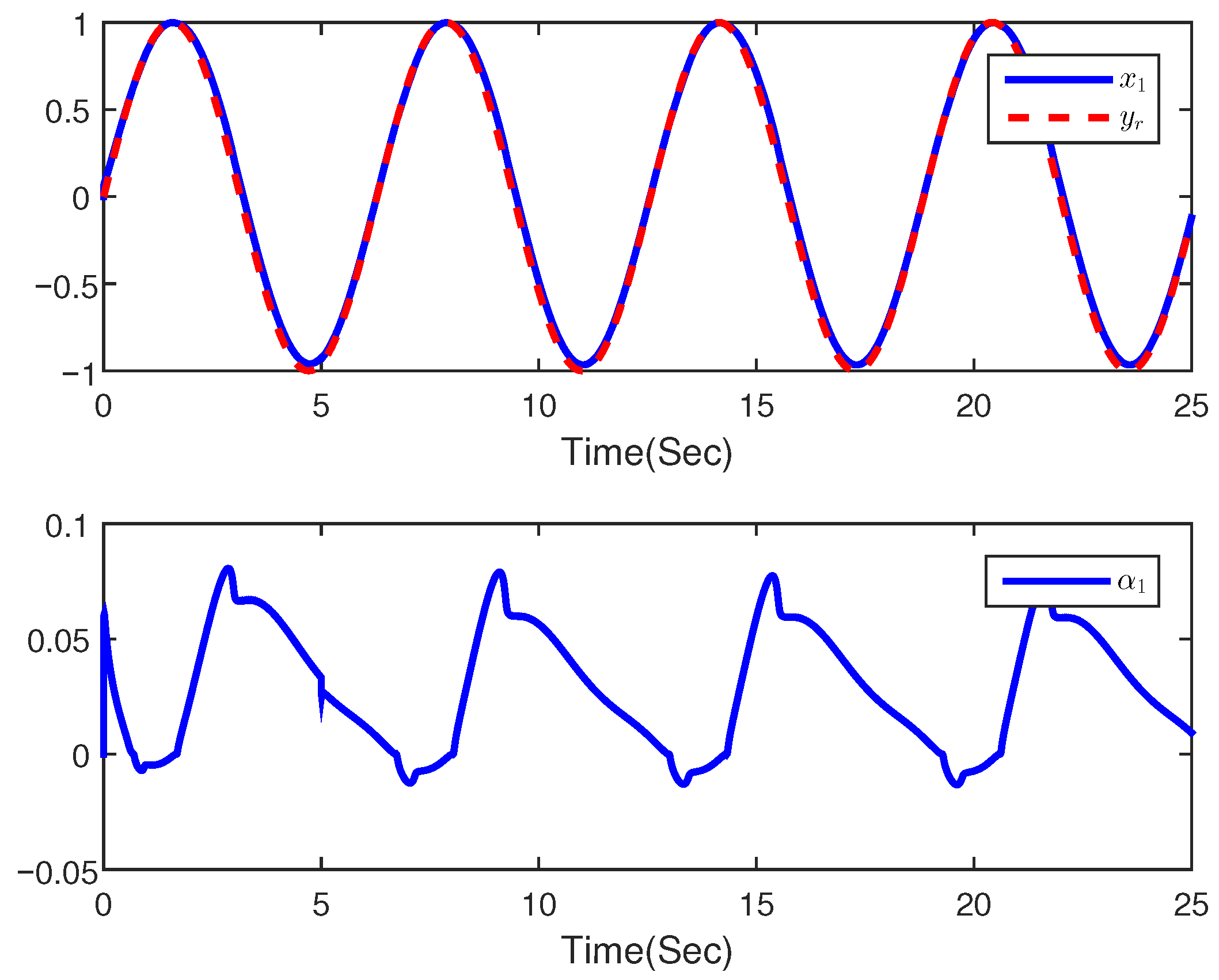
The FNS with PORP output signal can track the reference signal.

Proof. 

We define $\chi =min\left\{2{\sum }_{h=1}^n{c}_h,{\sum }_{h=1}^n{o}_h,o_c\right\}$, then we can obtain

$$\begin{array}{c}\hfill D^{\beta }{V}_n\le -\chi V_n+d_o\end{array}$$

(45)

According to Lemma 4, we have $V_n\left(t\right)\le \varsigma (V\left(0\right)+\frac{d_o}{\chi })$, where $\varsigma >0$ is a parameter. It is not difficult to get that ${\alpha }_1,\dots ,{\alpha }_n$, ${\tilde{\sigma }}_1,\dots ,{\tilde{\sigma }}_n$ and $\tilde{v}$ are bounded. Based on ${\widehat{\sigma }}_h={\sigma }_h-{\tilde{\sigma }}_h$ and $\widehat{v}=v-\tilde{v}$, we can obtain the boundedness of $\widehat{v}$ and ${\widehat{\sigma }}_h$, ($h=1,2,\dots ,n$). Obviously, the virtual law ${\lambda }_1$ is bounded due to the boundedness of ${\alpha }_1$ and ${\widehat{\sigma }}_1$. In addition, the boundedness of $x_2$ can be confirmed because of $x_2={\alpha }_2+{\lambda }_1$. Repeating the above analysis process, we can have that ${\lambda }_2,\dots ,{\lambda }_{n-1}$ and $x_3,\dots ,x_n$ are bounded. Then, we can say that all signals of the FNS with PORP are bounded. □

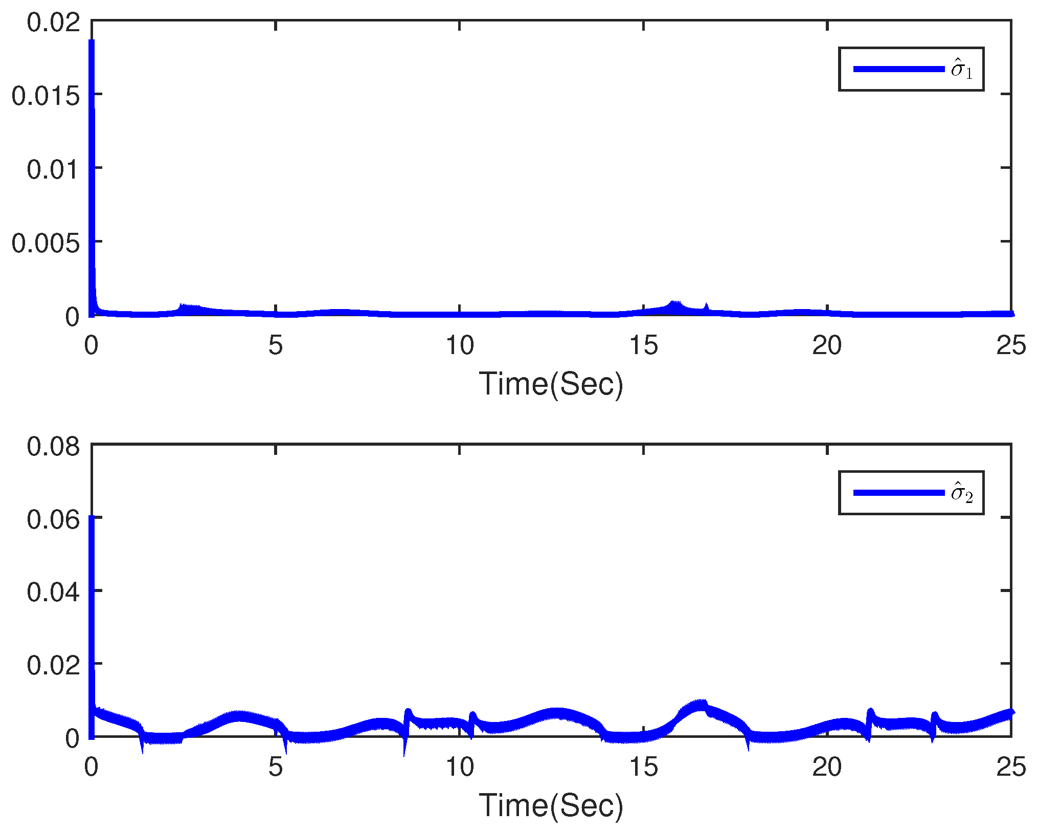
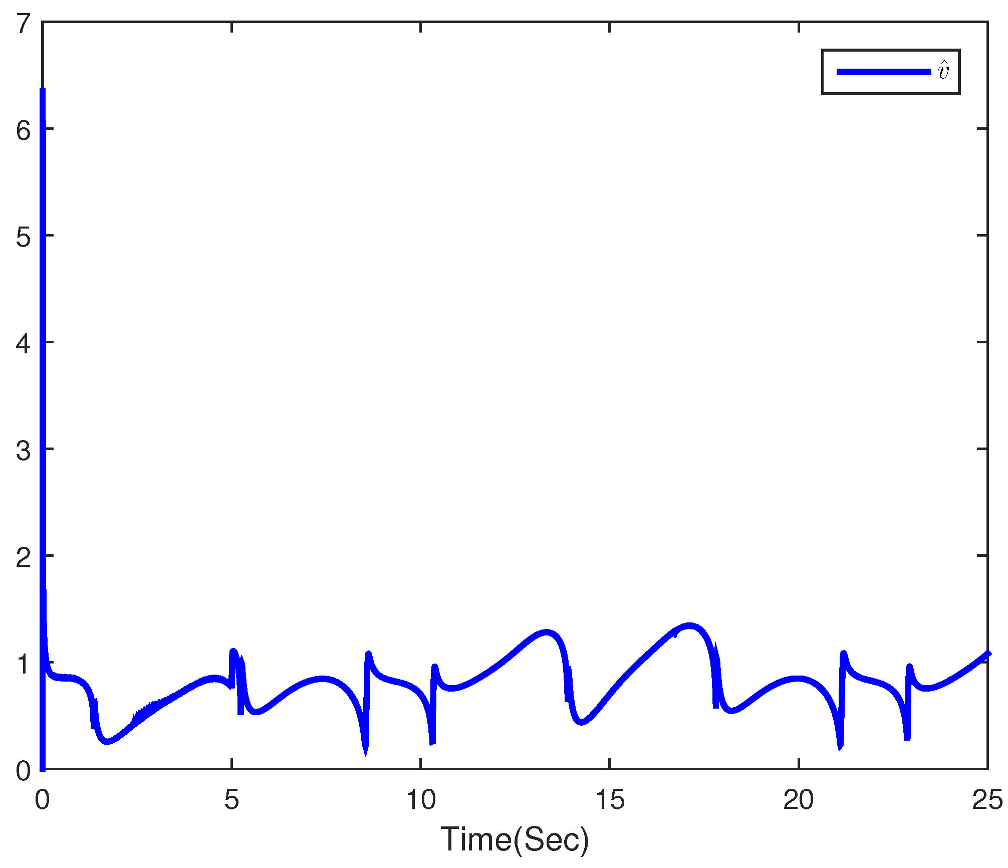
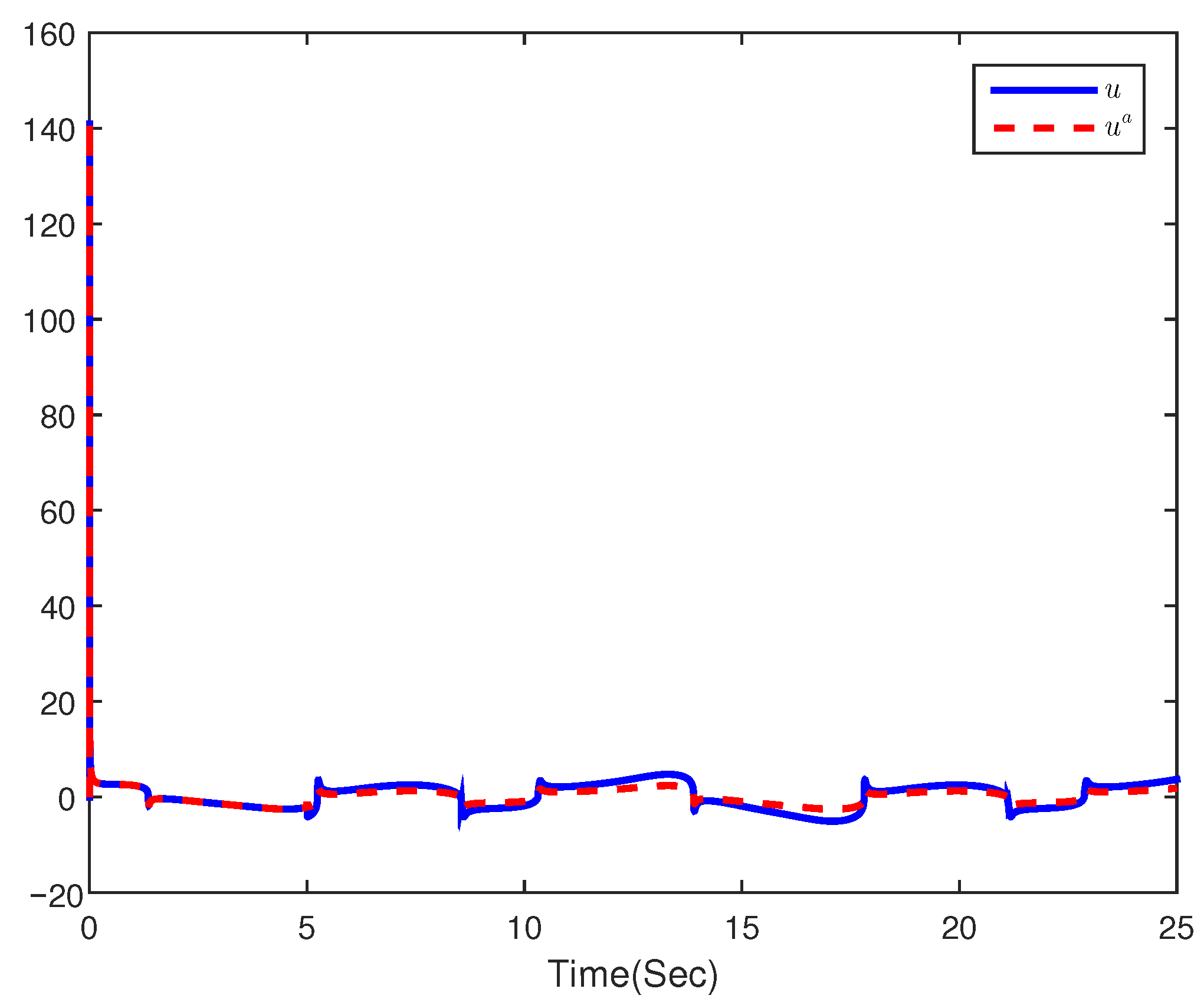
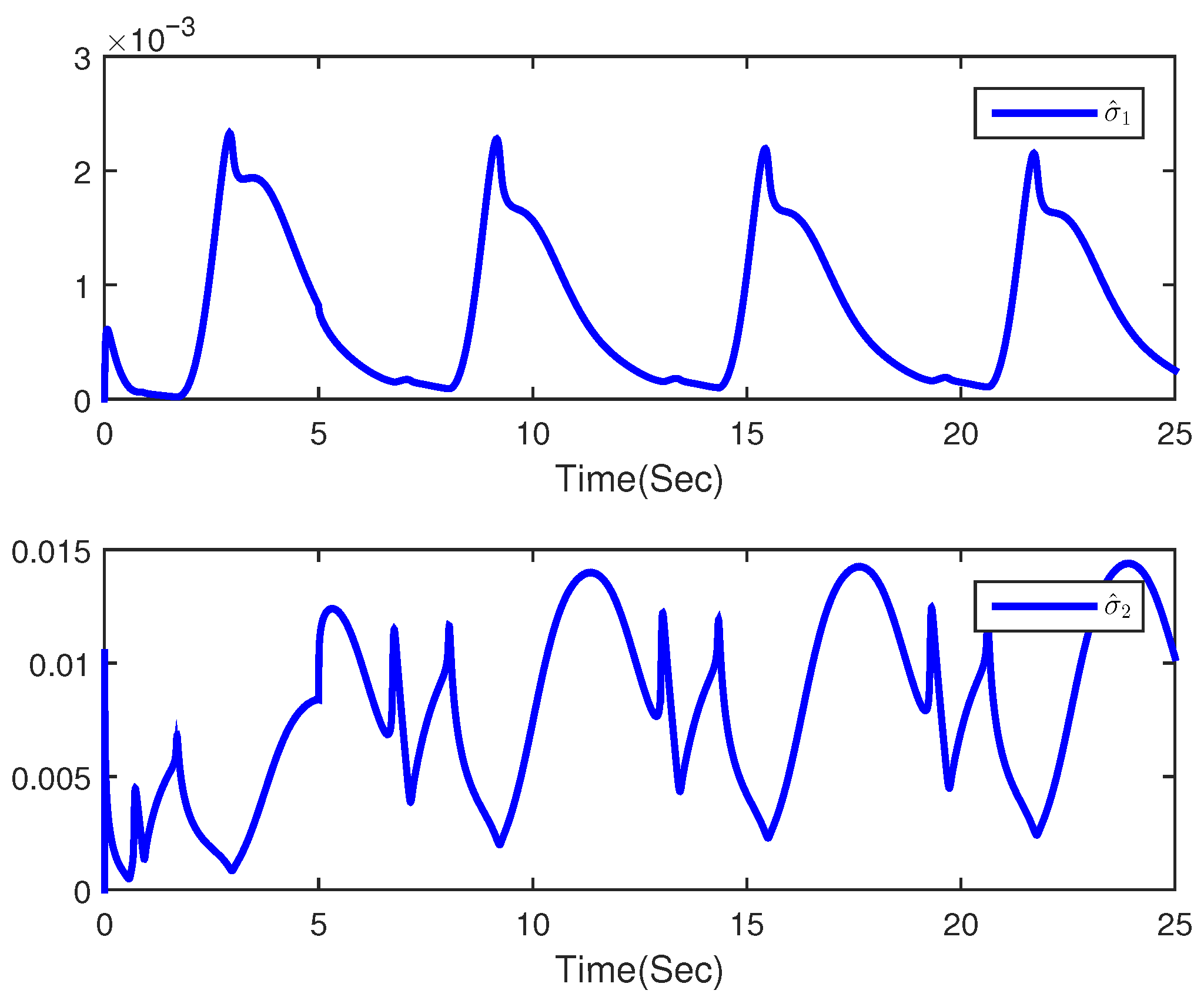
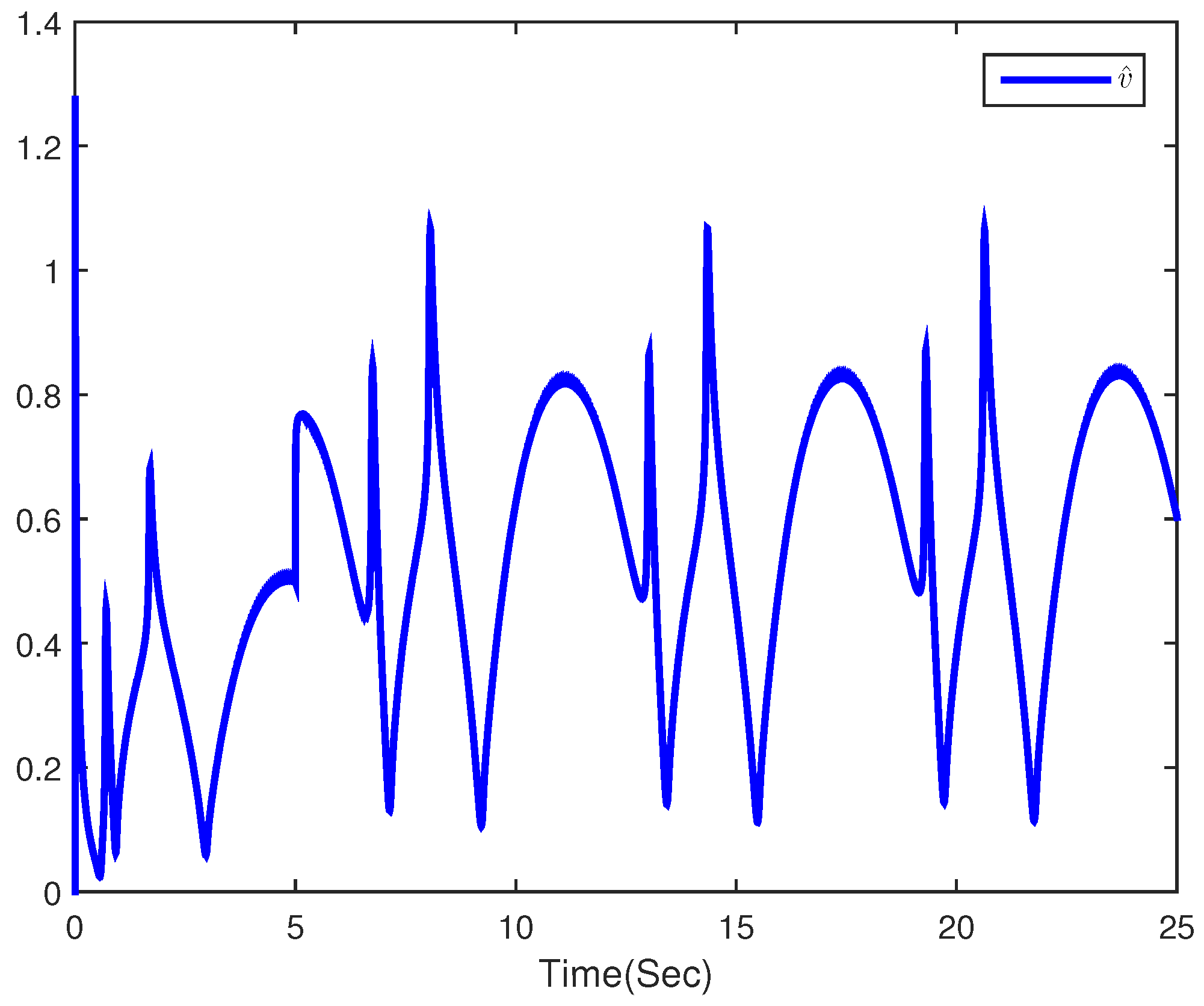
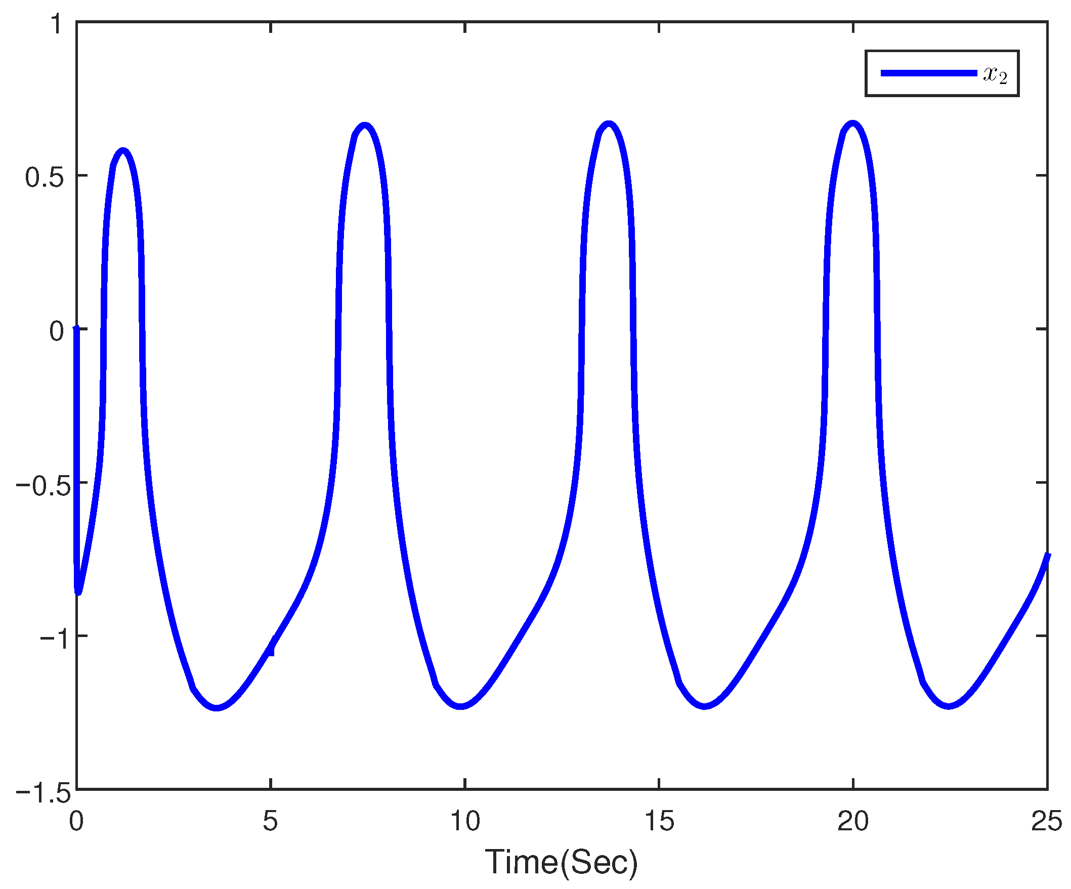
4. Simulation Example

Case 1: Consider a second-order FNS with PORP in this part

$$\left\{\begin{array}{c}{D}^{\beta }{x}_1=x_2^{{\xi }_1}+f_1\left({\overline{x}}_1\right),\hfill \\ D^{\beta }{x}_2=u+f_2\left({\overline{x}}_2\right),\hfill \\ y=x_1,\hfill \end{array}\right.$$

where $f_1\left({\overline{x}}_1\right)=sin\left(x_1\right)$, $f_2\left({\overline{x}}_2\right)=-x_1-x_2$ and ${\xi }_1=3$. The actuator fault can be expressed:

$$u^a=\left\{\begin{array}{c}u,t<t_n\hfill \\ \phi u+z\left(t\right),t\ge t_n\hfill \end{array}\right.$$

where $z\left(t\right)=0.01sin\left(t\right)$, $t_n=5s$.

The reference signal $y_r=sin\left(t\right)+cos\left(0.5t\right)$. The initial conditions are selected for case 1 as follows: ${[x_1\left(0\right),x_2\left(0\right),{\widehat{\sigma }}_1\left(0\right),{\widehat{\sigma }}_2\left(0\right),\widehat{v}\left(0\right)]}^T={[0,0,0,0,0]}^T$. The RBF NNs contain 11 nodes (${\overline{l}}_1={\overline{l}}_2=11$). ${\Phi }_i\left(P_i\right)={[s_{i1}\left(P_i\right),s_{i2}\left(P_i\right),\dots ,s_{i{\overline{l}}_i}\left(P_i\right)]}^T\in R^{{\overline{l}}_i}(i=1,2)$ where $s_{ij}\left(P_i\right)=exp-\frac{{(P_i-v_{ij})}^T(P_i-v_{ij})}{{\eta }_i^2}$ ($i=1,2,j=1,2,\dots ,{\overline{l}}_i$). In addition, $v_{1j}$ spaced in $[-5,5]\times [-5,5]$ and $v_{2j}$ spaced in $[-5,5]\times [-5,5]\times [-5,5]\times [-5,5]$. The widths are ${\eta }_i=\sqrt{2}$ for all.

The control goal of this paper is to design an adaptive neural FTC scheme which can ensure that the output signal y of the FNS with PORP can track the expected signal $y_r$. Given the virtual control law:

$$\begin{array}{c}\hfill {\lambda }_1=-{(c_1{\alpha }_1+\frac{1}{2b_1^2}{\alpha }_1{\widehat{\sigma }}_1{\Psi }_1^T{\Psi }_1)}^{\frac{1}{{\xi }_1}}\end{array}$$

(46)

The actual control u is defined as:

$$\begin{array}{c}\hfill u=\widehat{v}(-c_2{\alpha }_2-\frac{1}{2b_2^2}{\alpha }_2{\widehat{\sigma }}_2{\Psi }_2^T{\Psi }_2-z\left(t\right))\end{array}$$

(47)

In addition, the adaptive laws $D^{\beta }{\widehat{\sigma }}_h$ ($h=1,2$) and $D^{\beta }\widehat{v}$ can be selected as

$$\begin{array}{c}\hfill D^{\beta }{\widehat{\sigma }}_1=\frac{{\rho }_1}{2b_1^2}{\alpha }_1^2{\Psi }_1^T{\Psi }_1-o_1{\widehat{\sigma }}_1,\\ \hfill D^{\beta }{\widehat{\sigma }}_2=\frac{{\rho }_2}{2b_2^2}{\alpha }_2^2{\Psi }_2^T{\Psi }_2-o_2{\widehat{\sigma }}_2,\\ \hfill D^{\beta }\widehat{v}=-\gamma sign\left(\phi \right)\overline{u}{\alpha }_2-o_c\widehat{v}\end{array}$$

(48)

The above design parameters can be selected as follows: $c_1=50$, $c_2=10$, ${\rho }_1={\rho }_2=1$, $b_1=b_2=1$, $o_1=o_2=10$, $o_c=5$, and $\gamma =5$.

The simulation results can be exhibited in the Figure 1, Figure 2, Figure 3, Figure 4 and Figure 5. It is shown that the FNS with PORP output signal y follows the desired signal $y_r$, and the tracking error is near the origin in Figure 1. Figure 2 shows the curves ${\widehat{\sigma }}_1$ and ${\widehat{\sigma }}_2$ for the FNS with PORP. Figure 3 can exhibit the curve of $\widehat{v}$. In Figure 4, the designed control input u is stable and bounded. Figure 5 shows the state $x_2$ is bounded.

Case 2: Consider the following FNS with PORP in this part

$$\left\{\begin{array}{c}{D}^{\beta }{x}_1=x_2^{{\xi }_1}+f_1\left({\overline{x}}_1\right),\hfill \\ D^{\beta }{x}_2=u+f_2\left({\overline{x}}_2\right),\hfill \\ y=x_1,\hfill \end{array}\right.$$

where $f_1\left({\overline{x}}_1\right)=cos\left(x_1\right)$, $f_2\left({\overline{x}}_2\right)=sin\left(x_1\right)+x_2$ and ${\xi }_1=3$. The desired signal $y_r=sin\left(t\right)$. We take the same actuator fault, RBF NNs, the virtual control law ${\lambda }_1$, the actual control u, and the adaptive laws ($D^{\beta }{\widehat{\sigma }}_1,D^{\beta }{\widehat{\sigma }}_2,D^{\beta }\widehat{v}$) as Case 1. The initial conditions are selected for Case 2 as follows: ${[x_1\left(0\right),x_2\left(0\right),{\widehat{\sigma }}_1\left(0\right),{\widehat{\sigma }}_2\left(0\right),\widehat{v}\left(0\right)]}^T={[0,0,0,0,0]}^T$. However, the selection of parameters is different from Case 1. They are shown as: $c_1=c_2=20$, ${\rho }_1={\rho }_2=5$, $b_1=b_2=2$, $o_1=o_2=2$, $o_c=5$, and $\gamma =5$. The simulation results are presented in Figure 6, Figure 7, Figure 8, Figure 9 and Figure 10. The curve of output signal y and the desired signal $y_r$ and the curve of tracking error are shown in Figure 6. Figure 7 and Figure 8 show the curves ${\widehat{\sigma }}_1$, ${\widehat{\sigma }}_2$, and $\widehat{v}$. In Figure 9 and Figure 10, the designed control input u and the state $x_2$ are stable and bounded. According to the above two examples, we can clearly verify the effectiveness of the designed method.

5. Conclusions

In this paper, an adaptive neural FTC method was developed for the FNS with PORP. In particular, the FNSs subject to high-order terms are studied for the first time. The unknown functions of the systems have been approximated by RBF NNs. Under the frame of an adaptive approach and backstepping technology, the proposed controllers can ensure that all signals of an FNS with PORP are semi-global bounded and the tracking error is near the origin. The simulation example verifies the rationality of the developed control scheme.

References

1. Podlubny, I. Geometric and physical interpretation of fractional integration and fractional differentiation. Fract. Differ. Appl. 2001, 5, 230–237. [Google Scholar]
2. Shen, J.; Lam, J. Non-existence of finite-time stable equilibria in fractional-order nonlinear systems. Automatica 2004, 50, 547–551. [Google Scholar] [CrossRef]
3. Shen, J.; Lam, J. Stability and performance analysis for positive fractional-order systems with time-varying delays. IEEE Trans. Autom. Control 2016, 61, 2676–2681. [Google Scholar] [CrossRef]
4. Zhao, X.; Yin, Y.; Zheng, X. State-dependent switching control of switched positive fractional-order systems. ISA Trans. 2016, 62, 103–108. [Google Scholar] [CrossRef]
5. Wang, B.; Liu, Z.; Li, S.E.; Moura, S.J.; Peng, H. State-of-charge estimation for lithium-ion batteries based on a nonlinear fractional model. IEEE Trans. Control Syst. Technol. 2017, 25, 3–11. [Google Scholar] [CrossRef]
6. Zheng, S. Robust stability of fractional order system with general interval uncertainties. Syst. Control Lett. 2017, 99, 1–8. [Google Scholar] [CrossRef]
7. Li, Y.; Chen, Y.Q.; Podlubny, I. Mittag-Leffler stability of fractional order nonlinear dynamic systems. Automatica 2009, 45, 1965–1969. [Google Scholar] [CrossRef]
8. Aguila-Camacho, N.; Duarte-Mermoud, M.A.; Gallegos, J.A. Lyapunov functions for fractional order systems. Commun. Nonlinear Sci. Numer. 2014, 19, 2951–2958. [Google Scholar] [CrossRef]
9. Aghababa, M.P. Robust stabilization and synchronization of a class of fractional-order chaotic systems via a novel fractional sliding mode controller. Commun. Nonlinear Sci. Numer. Simul. 2012, 1, 2670–2681. [Google Scholar] [CrossRef]
10. Wei, Y.; Chen, Y.; Liang, S.; Wang, Y. A novel algorithm on adaptive backstepping control of fractional order systems. Neurocomputing 2015, 1, 395–402. [Google Scholar] [CrossRef]
11. Wei, Y.; Peter, T.; Yao, Z.; Wang, Y. Adaptive backstepping output feedback control for a class of nonlinear fractional order systems. Nonlinear Dyn. 2016, 1, 1047–1056. [Google Scholar] [CrossRef]
12. Trigeassou, J.C.; Maamri, N.; Sabatier, J.; Oustaloup, A. A Lyapunov approach to the stability of fractional differential equations. Signal Process. 2011, 1, 437–445. [Google Scholar] [CrossRef]
13. Yang, Z.; Zheng, S.; Liu, F.; Xie, Y. Adaptive output feedback control for fractional-order multi-agent systems. ISA Trans. 2019. [Google Scholar] [CrossRef] [PubMed]
14. Liang, B.Y.; Zheng, S.Q.; Ahn, C.K.; Liu, F. Adaptive fuzzy control for fractional-order interconnected systems with unknown control directions. IEEE Trans. Fuzzy Syst. 2022, 30, 75–87. [Google Scholar] [CrossRef]
15. Zhang, X.F.; Chen, Y.Q. Admissibility and robust stabilization of continuous linear singular fractional order systems with the fractional order α: The 0 < α < 1 case. ISA Trans. 2018, 82, 42–50. [Google Scholar] [PubMed]
16. Li, R.C.; Zhang, X.F. Adaptive sliding mode observer design for a class of T-S fuzzy descriptor fractional order systems. IEEE Trans. Fuzzy Syst. 2020, 28, 1951–1959. [Google Scholar] [CrossRef]
17. Zhang, X.F.; Zhao, Z.L. Normalization and stabilization for rectangular singular fractional order T-S fuzzy systems. Fuzzy Sets Syst. 2020, 38, 140–153. [Google Scholar] [CrossRef]
18. Zhang, X.F. Relationship between integer order systems and fractional order systems and Its two applications. IEEE-CAA J. Autom. Sin. 2018, 5, 539–643. [Google Scholar] [CrossRef]
19. Zhang, X.F.; Lin, C.; Chen, Y.Q.; Boutat, D. A unified framework of stability theorems for LTI fractional order systems with 0 < α < 2. IEEE Trans. Circuit Syst. II-Express 2020, 67, 3237–3241. [Google Scholar]
20. Zhang, X.F.; Huang, W.K. Adaptive neural network sliding mode control for nonlinear singular fractional order systems with mismatched uncertainties. Fractal Fract. 2020, 4, 50. [Google Scholar] [CrossRef]
21. Xie, R.M.; Guo, C.; Xie, X.J. Asymptotic tracking control of state-constrained nonlinear systems with time-varying powers. IEEE Trans. Cybern. 2022, 52, 4073–4078. [Google Scholar] [CrossRef] [PubMed]
22. Lin, W.; Qian, C. Adding one power integrator: A tool for global stabilization of high-order lower-triangular systems. Syst. Control Lett. 2000, 39, 339–351. [Google Scholar] [CrossRef]
23. Wang, H.Q.; Chen, M.; Liu, X.P. Fuzzy adaptive fixed-time quantized feedback control for a class of nonlinear systems. Acta Autom. Sin. 2021, 47, 2823–2830. [Google Scholar]
24. Wang, H.Q.; Xu, K.; Liu, X.P.; Qiao, J.F. Adaptive fuzzy fast finite-time dynamic surface tracking control for nonlinear systems. IEEE Trans. Circuits Syst. I Regul. Pap. 2021, 68, 4337–4348. [Google Scholar] [CrossRef]
25. Wang, H.Q.; Kang, S.J.; Zhao, X.D.; Xu, N.; Li, T.S. Command filter-based adaptive neural control design for nonstrict-feedback nonlinear systems with multiple actuator constraints. IEEE Trans. Cybern. 2021, 68, 1–10. [Google Scholar] [CrossRef]
26. Wang, H.Q.; Liu, P.X.P.; Bao, J.L.; Xie, X.J. Adaptive neural output-feedback decentralized control for large-scale nonlinear systems with stochastic disturbances. IEEE Trans. Neural Netw. Learn. Syst. 2020, 31, 972–983. [Google Scholar] [CrossRef]
27. Zhang, J.X.; Yang, G.H. Low-complexity tracking control of strict-feedback systems with unknown control directions. IEEE Trans. Autom. Control 2019, 64, 5175–5182. [Google Scholar] [CrossRef]
28. Zhang, J.X.; Wang, Q.G.; Ding, W. Global output-feedback prescribed performance control of nonlinear systems with unknown virtual control coefficients. IEEE Trans. Autom. Control 2021. Early Access. [Google Scholar] [CrossRef]
29. Wang, H.Q.; Ling, S.; Liu, P.X.P.; Li, Y.X. Control of high-order nonlinear systems under error-to-actuator based event-triggered framework. Int. J. Control 2022, 95, 2758–2770. [Google Scholar] [CrossRef]
30. Chen, C.L.P.; Wen, G.X.; Liu, Y.J.; Liu, Z. Observer-based adaptive backstepping consensus tracking control for high-order nonlinear semi-strict-feedback multiagent systems. IEEE Trans. Cybern. 2015, 46, 1591–1601. [Google Scholar] [CrossRef]
31. Jiang, M.M.; Xie, X.J.; Zhang, K. Finite-time stabilization of stochastic high-order nonlinear systems with FT-SISS inverse dynamics. IEEE Trans. Autom. Control 2019, 64, 313–320. [Google Scholar] [CrossRef]
32. Wang, H.Q.; Liu, S.W.; Wang, D.; Niu, B.; Chen, M. Adaptive neural tracking control of high-order nonlinear systems with quantized input. Neurocomputing 2021, 456, 156–167. [Google Scholar] [CrossRef]
33. Tong, S.; Li, K.; Li, Y. Robust fuzzy adaptive finite-time control for high-order nonlinear systems with unmodeled dynamics. IEEE Trans. Fuzzy Syst. 2021, 29, 1576–1598. [Google Scholar] [CrossRef]
34. Chen, M.; Tao, G. Adaptive fault-tolerant control of uncertain nonlinear large-scale systems with unknown dead zone. IEEE Trans. Cybern. 2015, 46, 1851–1862. [Google Scholar] [CrossRef]
35. Tang, X.; Tao, G.; Joshi, S.M. Adaptive actuator failure compensation for nonlinear mimo systems with an aircraft control application. Automatica 2007, 43, 1869–1883. [Google Scholar] [CrossRef]
36. Wang, W.; Wen, C. Adaptive actuator failure compensation control of uncertain nonlinear systems with guaranteed transient performance. Automatica 2010, 1, 2082–2091. [Google Scholar] [CrossRef]
37. Shen, Q.; Jiang, B.; Cocquempot, V. Fuzzy logic system-based adaptive fault-tolerant control for near-space vehicle attitude dynamics with actuator faults. IEEE Trans. Fuzzy Syst. 2012, 21, 289–300. [Google Scholar] [CrossRef]
38. Sun, K.K.; Liu, L.; Qiu, J.B.; Feng, G. Fuzzy adaptive finite-time fault-tolerant control for strict-feedback nonlinear systems. IEEE Trans. Fuzzy Syst. 2021, 29, 786–796. [Google Scholar] [CrossRef]
39. Yang, H.Y.; Jiang, Y.C.; Shen, Y. Adaptive fuzzy fault-tolerant control for markov jump systems with additive and multiplicative actuator faults. IEEE Trans. Fuzzy Syst. 2021, 29, 772–785. [Google Scholar] [CrossRef]
40. Zhang, J.X.; Yang, G.H. Fault-tolerant output-constrained control of unknown Euler-Lagrange systems with prescribed tracking accuracy. Automatica 2020, 111, 108606. [Google Scholar] [CrossRef]
41. Zhang, X.F.; Huang, W.K.; Wang, Q.G. Robust H-infinity adaptive sliding mode fault tolerant control for T-S fuzzy fractional order systems with mismatched disturbances. IEEE Trans. Circuit Syst. I-Regul. Pap. 2021, 68, 1297–1307. [Google Scholar] [CrossRef]
42. Martinez-Fuentes, O.; Melendez-Vazquez, F.; Martinez-Guerra, R. Fractional-order nonlinear systems with fault tolerance. In Proceedings of the 2018 Annual American Control Conference (ACC), Milwaukee, WI, USA, 27–29 June 2018. [Google Scholar]
43. Li, X.M.; Zhan, Y.L.; Tong, S.C. Adaptive neural network decentralized fault-tolerant control for nonlinear interconnected fractional-order systems. Neurocomputing 2022, 488, 14–22. [Google Scholar] [CrossRef]
44. Hu, X.R.; Song, Q.; Ge, M.; Li, R.M. Fractional-order adaptive fault-tolerant control for a class of general nonlinear systems. Nonlinear Dyn. 2020, 101, 379–392. [Google Scholar] [CrossRef]
45. Benchaita, H.; Ladaci, S. Fractional adaptive SMC fault tolerant control against actuator failures for wing rock supervision. Aerosp. Sci. Technol. 2021, 114, 106745. [Google Scholar] [CrossRef]
46. Zhou, J.; Wen, C.Y. Adaptive Backstepping Control of Uncertain Systems: Nonsmooth Nonlinearities, Interactions or Time-Variations; Springer: Berlin, Germany, 2008. [Google Scholar]
47. Qian, C.; Lin, W. Practical output tracking of nonlinear systems with uncontrollable unstable linearization. IEEE Trans. Autom. Control 2021, 47, 21–36. [Google Scholar] [CrossRef]
48. Podlubny, I. Fractional Differential Equations; Academic Press: San Diego, CA, USA, 1999. [Google Scholar]
49. Liu, S.W.; Wang, H.Q.; Li, T.S. Adaptive composite dynamic surface neural control for nonlinear fractional-order systems subject to delayed input. ISA Trans. 2022, in press. [Google Scholar] [CrossRef]
50. Yang, B.; Lin, W. Homogeneous observers, iterative design, and global stabilization of high-order nonlinear systems by smooth output feedback. IEEE Trans. Autom. Control 2004, 49, 1069–1080. [Google Scholar] [CrossRef]
51. Sanner, R.M.; Slotine, J.E. Gaussian networks for direct adaptive control. IEEE Trans. Neural Netw. 1992, 3, 837–863. [Google Scholar] [CrossRef]
Figure 1. The output signal y and the desired signal y r , and the tracking error α 1 (Case 1).
Fractalfract 06 00622 g001
Figure 2. The curves of σ ^ 1 and σ ^ 2 (Case 1).
Fractalfract 06 00622 g002
Figure 3. The curve of v ^ (Case 1).
Fractalfract 06 00622 g003
Figure 4. The control input u a (Case 1).
Fractalfract 06 00622 g004
Figure 5. The system state x 2 (Case 1).
Fractalfract 06 00622 g005
Figure 6. The output signal y and the desired signal y r , and the tracking error α 1 (Case 2).
Fractalfract 06 00622 g006
Figure 7. The curves of σ ^ 1 and σ ^ 2 (Case 2).
Fractalfract 06 00622 g007
Figure 8. The curve of v ^ (Case 2).
Fractalfract 06 00622 g008
Figure 9. The control input u a (Case 2).
Fractalfract 06 00622 g009
Figure 10. The system state x 2 (Case 2).
Fractalfract 06 00622 g010
Publisher’s Note: MDPI stays neutral with regard to jurisdictional claims in published maps and institutional affiliations.