General Methods to Synchronize Fractional Discrete Reaction–Diffusion Systems Applied to the Glycolysis Model

Abstract

Because they are useful for both enabling numerical simulations and containing well-defined physical phenomena, discrete fractional reaction–diffusion models have attracted a great deal of interest from academics. Within the family of fractional reaction–diffusion models, a discrete form is examined in detail in this study. Furthermore, we investigate the complex synchronization dynamics of a suggested discrete master–slave reaction–diffusion system using the accuracy of linear control techniques combined with a fractional discrete Lyapunov approach. This study’s deviation from the behavior of equivalents with integer orders makes it very fascinating. Like the non-local nature inherent in Caputo fractional derivatives, it creates a memory Lyapunov function that is closely linked to the historical background of the system. The investigation provides a strong basis to the theoretical results.

1. Introduction

In recent years, researchers have delved deep into the fascinating realm of reaction–diffusion equations and their applications, guided by a commitment to explore novel frontiers [1,2,3]. Conventional literature has extended the boundaries by applying these equations to unconventional domains, focusing on harnessing their power in fields such as tissue engineering and material science [4,5,6]. Utilizing innovative mathematical models, several works have explored how reaction–diffusion principles can influence the growth of biological tissues and the self-assembly of materials with tailored properties.

Fractional calculus, encompassing non-integer-order derivatives and integrals, has redefined the modeling of diffusion processes [7,8]. Fractional reaction–diffusion equations incorporate these fractional derivatives, yielding a more accurate portrayal of intricate diffusion behaviors that deviate from linear or exponential trends. These equations transcend the boundaries of classical reaction–diffusion frameworks, accommodating phenomena such as subdiffusion and superdiffusion, which are prevalent in a spectrum of natural and artificial systems. Fractional reaction–diffusion equations find applications in modeling ecological patterns and population dynamics [9,10,11,12]. They offer a nuanced perspective on species interactions, spatial distribution, and the persistence of species in heterogeneous environments.

Merging fractional calculus with discrete mathematics gives rise to fractional discrete equations. These equations accommodate the inherently discrete nature of many processes while embracing the intricacies of fractional dynamics, resulting in models that describe phenomena where both discrete steps and fractional derivatives are integral to understanding [13,14,15,16,17,18]. Meanwhile, fractional discrete reaction–diffusion equations offer a unique framework for modeling intricate patterns, interactions, and diffusion processes that exist in both discrete and fractional dimensions [19,20]. By merging the concepts of reaction kinetics, fractional calculus, and discrete dynamics, these equations provide a comprehensive way to study phenomena where discrete entities interact and diffuse while accounting for the complexities of fractional-order behaviors. In the research presented in [21], A fractional discrete reaction–diffusion Glycolysis model’s local and global stability were carefully investigated. Furthermore, [22] explored the FitzHugh–Nagumo model’s dynamics as expressed by fractional difference equations. Furthermore, fractional-order discrete-time reaction–diffusion systems were presented and their dynamic behavior was examined by [23]. Furthermore, the work in [24] concentrated on talking about a fractional discrete reaction–diffusion epidemic model’s stability.

Synchronization of fractional-order systems is an interesting and complex topic. It involves studying the behavior of multiple fractional-order systems that are coupled together, causing their dynamics to become correlated or synchronized. The study, which is cited as [25], used an adaptive sliding mode control technique based on a finite-time scheme to study projective synchronization of a fractional reaction–diffusion systems. Turning now to the work reported in [26], this research investigated the application of these synchronization concepts to different biochemical models, with a focus on the global synchronization of fractional reaction–diffusion systems. Furthermore, a hybrid technique for synchronizing two reaction–diffusion systems was proposed by the study reported in [27], which also gave application scenarios in certain chemical models. Additionally, the work discussed in [28] addressed the problem of synchronization for a particular class of fractional-order spatiotemporal partial differential systems by applying a fractional Lyapunov technique. The synchronization of such systems can exhibit different patterns compared to classical integer-order systems. Synchronization within fractional discrete equations entails achieving coordinated states among fractional discrete entities over discrete time steps [29,30,31]. The study of synchronization dynamics in fractional discrete equations involves understanding the conditions that foster synchronization, unveiling the emergence of synchronized states and quantifying the degree of synchronization within this novel framework. The fusion of fractional calculus and discrete reaction–diffusion dynamics introduces a fresh layer of complexity to synchronization studies [32]. Fractional discrete entities, connected by fractional diffusion, interact through reaction kinetics. Synchronization phenomena within this framework lead to intriguing patterns and behaviors that are shaped by both fractional calculus and discrete dynamics. Fractional discrete reaction–diffusion equations pave the way for modeling biological tissues with non-classical diffusion properties. Synchronization within these equations contributes to understanding synchronized patterns that emerge in biological contexts.

To the best of the authors’ knowledge, this work is the first attempt to look at the elements of discrete, generalized fractional reaction–diffusion systems that deal with synchronization and control. This first emphasis led to a detailed investigation of how to attain perfect synchronization in coupled discrete generalized fractional reaction–diffusion systems. The study discretized the systems under consideration using the L1 finite difference scheme and the second-order central difference scheme and then applied the fractional Lyapunov technique to incorporate both nonlinear and linear control approaches. Moreover, the Glycolysis model, a chaotic reaction–diffusion model, was analyzed using the theoretical results and control methodologies. Discrete system formulations were given together with matching simulations to show how the developed approaches may be used in real-world scenarios. The paper’s structure is delineated as follows: Section 2 commences by introducing generalized discrete fractional reaction–diffusion systems and fundamental concepts related to discrete fractional calculus. In Section 3, an investigation unfolds into the synchronization of the considered master–slave system through the utilization of nonlinear control techniques. Subsequently, Section 4 tackles the synchronization challenge by employing distinctive linear control strategies, accompanied by demonstrations of convergence grounded in a relevant Lyapunov functional. In Section 5, we shift focus to an applied context where we analytically and numerically derive control laws to attain synchronization between the master–slave systems of two dimensions of the fractional discrete reaction–diffusion Glycolysis model.

2. Basic Tools and Problem Formulation

In this study, we explore master–slave systems employing two widely recognized techniques: the second-order difference scheme and the $L1$ finite difference scheme. To achieve this, we discretize the fractional reaction–diffusion Equation (1) using the discretization method outlined by Wu et al. [33].

$$\left\{\begin{array}{c}{\displaystyle \frac{\partial \mathfrak{z}}{\partial t}}=\mathfrak{k}\Delta \mathfrak{z},t>0,\mathsf{x}\in \Omega ,\hfill \\ {\partial }_{\mathsf{x}}\mathfrak{z}=0,t>0,\mathsf{x}\in \partial \Omega ,\hfill \\ \mathfrak{z}(0,\mathsf{x})={\mathfrak{z}}_0\left(\mathsf{x}\right),\mathsf{x}\in \Omega .\hfill \end{array}\right.$$

(1)

Utilizing the framework presented in Equation (1) and drawing upon the discretization methodology introduced in references [33,34], we navigate the interval $\mathsf{x}\in [0,L]$. Within this context, as ${\mathsf{x}}_{i+1}={\mathsf{x}}_i+d_x$ for $i=0,\dots ,m$, we proceed by employing the central difference formula to estimate $\frac{{\partial }^2\mathfrak{z}(\mathsf{x},t)}{\partial {\mathsf{x}}^2}$.

$$\left\{\begin{array}{c}{\displaystyle \frac{{\partial }^2\mathfrak{z}(\mathsf{x},t)}{\partial {\mathsf{x}}^2}}\approx {\displaystyle \frac{{\mathfrak{z}}_{i+1}\left(t\right)-2{\mathfrak{z}}_i\left(t\right)+{\mathfrak{z}}_{i-1}\left(t\right)}{d_{\mathsf{x}}^2}},\hfill \end{array}\right.$$

(2)

Applying the characterization of the second-order difference operator of ${\mathfrak{z}}_i$ as delineated in reference [35], whereby

$$\begin{array}{c}\hfill {\Delta }^2\chi \left(\mathsf{\ell }\right)=\chi (\mathsf{\ell }+2)-2\chi (\mathsf{\ell }+1)+\chi \left(\mathsf{\ell }\right),\mathsf{\ell }\in \mathbb{N},\end{array}$$

(3)

the subsequent approximations arise from our analysis.

$$\left\{\begin{array}{c}{\displaystyle \frac{{\partial }^2\mathfrak{z}(\mathsf{x},t)}{\partial {\mathsf{x}}^2}}\approx {\displaystyle \frac{{\Delta }^2{\mathfrak{z}}_{i-1}\left(t\right)}{d_{\mathsf{x}}^2}},\hfill \end{array}\right.$$

(4)

Consequently, we can establish a connection between the aforementioned model described in references [33,34].

$${}_{\hslash }^C\Delta t_0{\mathfrak{z}}_i\left(t\right)=\mathfrak{e}{\Delta }^2{\mathfrak{z}}_{i-1}(t+\hslash ),\mathfrak{e}={\displaystyle \frac{\mathfrak{k}}{{\Delta }_{\mathsf{x}}^2}}.$$

(5)

Under the context of periodic boundary conditions,

$${\mathfrak{z}}_0\left(t\right)={\mathfrak{z}}_m\left(t\right),{\mathfrak{z}}_1\left(t\right)={\mathfrak{z}}_{m+1}\left(t\right).$$

(6)

The characterization of the Caputo ℏ-difference operator is outlined by the following definition

Definition 1 

([36,37]). The expression for the Caputo ℏ-difference operator is given by

$$\begin{array}{c}\hfill {}_{\hslash }^C{\Delta }_a^{\xi }\chi \left(t\right)={}_{\hslash }{\Delta }_{\mathfrak{a}}^{-(n-\xi )}{\Delta }_{\hslash }^n\chi \left(t\right),t\in {(\hslash \mathbb{N})}_{\mathfrak{a}+\xi \hslash },0<\xi <1,\end{array}$$

(7)

The ξ-th order ℏ-sum is defined as

$$\begin{array}{c}\hfill {}_{\hslash }{\Delta }_{\mathfrak{a}}^{-\xi }\chi \left(t\right)=\frac{\hslash }{\Gamma \left(\xi \right)}\sum _{\frac{t}{\hslash }-\xi }^{s=\frac{\mathfrak{a}}{\hslash }}{(t-\sigma (s\hslash ))}^{(\xi -1)}\chi (s\hslash ),\sigma (s\hslash )=(s+1)\hslash .\end{array}$$

(8)

along with the set ${(\hslash \mathbb{N})}_{\mathfrak{a}+\xi \hslash }$ defined by

$${(\hslash \mathbb{N})}_{\mathfrak{a}+\xi \hslash }=\{\mathfrak{a}+(1-\xi )\hslash ,\mathfrak{a}+(2-\xi )\hslash ,\dots \},$$

Extensive research has been conducted on models involving chaotic fractional-order anomalous diffusion. Notably, the exploration of synchronization within these systems has garnered significant attention. In fact, the investigation of synchronization dynamics was and remains a vital subject of inquiry. An illustrative example can be found in the work of [12], where they scrutinized the synchronization of a specific class of reaction–diffusion models (9) utilizing fractional-order formulations.

$$\left\{\begin{array}{c}{}_0^C{D}_t^{\delta }\mathfrak{z}={\mathfrak{k}}_1\Delta \mathfrak{z}+\mathfrak{a}\mathfrak{z}+{\chi }_1(\mathfrak{z},\mathfrak{w}),\hfill \\ {}_0^C{D}_t^{\delta }\mathfrak{w}={\mathfrak{k}}_2\Delta \mathfrak{w}+\mathfrak{b}\mathfrak{w}+{\chi }_2(\mathfrak{z},\mathfrak{w}).\hfill \end{array}\right.$$

(9)

where ${(\mathfrak{z}(\mathsf{x},t),\mathfrak{w}(\mathsf{x},t))}^T$ are the corresponding states, $\mathsf{x}\in \Omega$ is a bounded domain in ${\mathbb{R}}^n$ with smooth boundary $\partial \Omega$, and ${\mathfrak{k}}_1,{\mathfrak{k}}_2,\mathfrak{a},\mathfrak{b}\in \mathbb{R}$, ${\chi }_1,{\chi }_2$, are nonlinear continuous functions.

Thus, proceeding according to the previously outlined procedure, consider the discrete fractional reaction–diffusion master–slave system based on the framework presented in Equation (9).

$$\begin{array}{c}\hfill \mathrm{Master}\mathrm{system}\left\{\begin{array}{c}{}_{\hslash }^C{\Delta }_{t_0}^{\xi }{\mathfrak{z}}_i\left(t\right)={\mathfrak{e}}_1{\Delta }^2{\mathfrak{z}}_{i-1}(t+\hslash \xi )+\mathfrak{a}{\mathfrak{z}}_i(t+\hslash \xi )+{\chi }_1({\mathfrak{z}}_i(t+\hslash \xi ),{\mathfrak{w}}_i(t+\hslash \xi )),\hfill \\ {}_{\hslash }^C{\Delta }_{t_0}^{\xi }{\mathfrak{w}}_i\left(t\right)={\mathfrak{e}}_2{\Delta }^2{\mathfrak{w}}_{i-1}(t+\hslash \xi )+\mathfrak{b}{\mathfrak{w}}_i(t+\hslash \xi )+{\chi }_2({\mathfrak{z}}_i(t+\hslash \xi ),{\mathfrak{w}}_i(t+\hslash \xi )),\hfill \end{array}\right.\end{array}$$

(10)

$$\begin{array}{c}\hfill \mathrm{Slave}\mathrm{system}\left\{\begin{array}{c}{}_{\hslash }^C{\Delta }_{t_0}^{\xi }{\mathfrak{Z}}_i\left(t\right)=m_1{\Delta }^2{\mathfrak{Z}}_{i-1}(t+\hslash \xi )+\mathfrak{a}{\mathfrak{Z}}_i(t+\hslash \xi )+{\chi }_1({\mathfrak{Z}}_i(t+\hslash \xi ),{\mathfrak{W}}_i(t+\hslash \xi ))\hfill \\ +W_1\left(t\right)\hfill \\ {}_{\hslash }^C{\Delta }_{t_0}^{\xi }{\mathfrak{W}}_i\left(t\right)={\mathfrak{e}}_2{\Delta }^2{\mathfrak{W}}_{i-1}(t+\hslash \xi )+\mathfrak{b}{\mathfrak{W}}_i(t+\hslash \xi )+{\chi }_2({\mathfrak{Z}}_i(t+\hslash \xi ),{\mathfrak{W}}_i(t+\hslash \xi ))\hfill \\ +W_2\left(t\right),\hfill \end{array}\right.\end{array}$$

(11)

where $m_i={\displaystyle \frac{{\mathfrak{k}}_i}{d_{\mathsf{x}}^2}},i=1,2.$ With the periodic boundary conditions

$$\begin{array}{c}\hfill \left\{\begin{array}{c}{\mathfrak{z}}_0\left(t\right)={\mathfrak{z}}_m\left(t\right),{\mathfrak{z}}_1\left(t\right)={\mathfrak{z}}_{m+1}\left(t\right),{\mathfrak{Z}}_0\left(t\right)={\mathfrak{Z}}_m\left(t\right),{\mathfrak{Z}}_1\left(t\right)={\mathfrak{Z}}_{m+1}\left(t\right),\hfill \\ {\mathfrak{w}}_0\left(t\right)={\mathfrak{w}}_m\left(t\right),{\mathfrak{w}}_1\left(t\right)={\mathfrak{w}}_{m+1}\left(t\right),{\mathfrak{W}}_0\left(t\right)={\mathfrak{W}}_m\left(t\right),{\mathfrak{W}}_1\left(t\right)={\mathfrak{W}}_{m+1}\left(t\right),\hfill \end{array}\right.\end{array}$$

(12)

and the initial condition

$$\left\{\begin{array}{c}{\mathfrak{z}}_i\left(t_0\right)={\mathfrak{H}}_1\left({\mathsf{x}}_i\right)\ge 0,{\mathfrak{Z}}_i\left(t_0\right)={\mathfrak{H}}_2\left({\mathsf{x}}_i\right)\ge 0,\hfill \\ {\mathfrak{w}}_i\left(t_0\right)={\mathfrak{G}}_1\left({\mathsf{x}}_i\right)\ge 0,{\mathfrak{W}}_i\left(t_0\right)={\mathfrak{G}}_2\left({\mathsf{x}}_i\right)\ge 0,\hfill \end{array}\right.$$

Minimizing and eventually eliminating the difference between the slave and master systems is the goal of synchronization, as elucidated by

$$e_i=(e_{1i},e_{2i})=({\mathfrak{Z}}_i-{\mathfrak{z}}_i,{\mathfrak{W}}_i-{\mathfrak{w}}_i),$$

(13)

In essence, achieving absolute synchronization within the master–slave systems (10) and (11) necessitates assessing the asymptotic stability of the zero solution within the synchronization error system delineated by Equation (13).

Upon substituting Equation (20) into the error system presented in Equation (13), we obtain

$$\left\{\begin{array}{c}{}_{\hslash }^C\Delta t_0{e}_{1i}\left(t\right)=m_1{\Delta }^2{e}_{1,i-1}(t+\hslash )+\mathfrak{a}{e}_{1i}(t+h)+{\chi }_1({\mathfrak{Z}}_i(t+\hslash \xi ),{\mathfrak{W}}_i(t+\hslash \xi ))\hfill \\ -{\chi }_1({\mathfrak{z}}_i(t+\hslash \xi ),{\mathfrak{w}}_i(t+\hslash \xi ))+W_1\left(t\right),\hfill \\ {}_{\hslash }^C\Delta t_0{e}_{2i}\left(t\right)=m_2{\Delta }^2{e}_{2,i-1}(t+\hslash )+\mathfrak{b}{e}_{2i}(t+\hslash )+{\chi }_2({\mathfrak{Z}}_i(t+\hslash \xi ),{\mathfrak{W}}_i(t+\hslash \xi ))\hfill \\ -{\chi }_2({\mathfrak{z}}_i(t+\hslash \xi ),{\mathfrak{w}}_i(t+\hslash \xi ))+W_2\left(t\right).\hfill \end{array}\right.$$

(14)

Prior to advancing with our discussion, it is imperative to lay the groundwork by introducing and elaborating upon fundamental concepts related to the asymptotic stability of the error system.

Theorem 1 

([36]). The equilibrium point within system (14) achieves asymptotic stability under the condition that there is a positively distinct and decreasing function of scale Ł satisfying: ${\hslash }^C\Delta {t_0}^{\xi }Ł\left(t\right)\le 0$.

We also have the following important inequality:

Lemma 1 

([36]). The following inequality holds:

$$\begin{array}{c}\hfill {}_{\hslash }^C{\Delta }_{\mathfrak{a}}^{\xi }{\chi }^2\left(t\right)\le 2\chi {(t+\xi \hslash )}_h^C{\Delta }_{\mathfrak{a}}^{\xi }\chi \left(t\right),t\in {(\hslash \mathbb{N})}_{\mathfrak{a}+\xi \hslash },\end{array}$$

(15)

Theorem 2 

([38]). The summation using the parts formula for two functions χ and $\mathfrak{y}$, both defined on $\mathbb{N}$, with $\mathfrak{a}$ and $\mathfrak{b}$ belonging to $\mathbb{N}$, is expressed as follows:

$$\begin{array}{cc}\hfill & \sum _{𝚥=\mathfrak{a}}^{\mathfrak{b}-1}\chi \left(𝚥\right)\Delta \mathfrak{y}\left(𝚥\right)={\left.\chi \left(𝚥\right)\mathfrak{y}\left(𝚥\right)\right|}_{\mathfrak{a}}^{\mathfrak{b}}-\sum _{𝚥=\mathfrak{a}}^{\mathfrak{b}-1}\mathfrak{y}(𝚥+1)\Delta \chi \left(𝚥\right),\hfill \end{array}$$

(16)

$$\begin{array}{cc}\hfill & \sum _{𝚥=\mathfrak{a}}^{\mathfrak{b}-1}\chi (𝚥+1)\Delta \mathfrak{y}\left(𝚥\right)={\left.\chi \left(𝚥\right)\mathfrak{y}\left(𝚥\right)\right|}_{\mathfrak{a}}^{\mathfrak{b}}-\sum _{𝚥=\mathfrak{a}}^{\mathfrak{b}-1}\mathfrak{y}\left(𝚥\right)\Delta \chi \left(𝚥\right).\hfill \end{array}$$

(17)

while the definition of the forward difference operator Δ is

$$\begin{array}{c}\hfill \Delta \chi \left(𝚥\right)=\chi (𝚥+1)-\chi \left(𝚥\right).\end{array}$$

(18)

Definition 2. 

The master and slave systems provided in (10) and (11) are deemed fully synchronized if condition (19) is met.

$$\underset{t\to +\infty }{lim}\parallel e_i\left(t\right)\parallel =0.$$

(19)

3. Nonlinear Approach

Within this section, we delineate the task of exerting control over the interconnected master and slave systems, as depicted in Equations (10) and (11), employing nonlinear control strategies.

Theorem 3. 

Complete synchronization is achieved between the master system (10) and the slave system (11) through the utilization of the subsequent nonlinear control law:

$$\left\{\begin{array}{c}{W}_1\left(t\right)=(\mathfrak{a}-c_1)e_{1i}(t+h)+{\chi }_1({\mathfrak{Z}}_i(t+\hslash \xi ),{\mathfrak{W}}_i(t+\hslash \xi ))-{\chi }_1({\mathfrak{z}}_i(t+\hslash \xi ),{\mathfrak{w}}_i(t+\hslash \xi )),\hfill \\ W_2\left(t\right)=(\mathfrak{b}-{\mathfrak{c}}_2)e_{2i}(t+\hslash )+{\chi }_2({\mathfrak{Z}}_i(t+\hslash \xi ),{\mathfrak{W}}_i(t+\hslash \xi ))-{\chi }_2({\mathfrak{z}}_i(t+\hslash \xi ),{\mathfrak{w}}_i(t+\hslash \xi )).\hfill \end{array}\right.$$

(20)

where $A=diag{\left(a_{ij}\right)}_{2\times 2}$ and the control matrix $C=diag{\left(c_{ij}\right)}_{2\times 2}$ is chosen in a manner that ensures the matrix $C-A$ is positive definite.

Proof. 

Substituting the control law (20) into the system (14) yields the subsequent set of equations:

$$\left\{\begin{array}{c}{}_{\hslash }^C\Delta t_0{e}_{1i}\left(t\right)=m_1{\Delta }^2{e}_{1,i-1}(t+\hslash )+(\mathfrak{a}-c_1)e_{1i}(t+h),\hfill \\ {}_{\hslash }^C\Delta t_0{e}_{2i}\left(t\right)=m_2{\Delta }^2{e}_{2,i-1}(t+\hslash )+(\mathfrak{b}-{\mathfrak{c}}_2)e_{2i}(t+\hslash ).\hfill \end{array}\right.$$

(21)

Constructing a Lyapunov function of the form

$$L\left(t\right)={\displaystyle \frac{1}{2}}\sum _{i=1}^m{e}_{1i}^2\left(t\right)+e_{2i}^2\left(t\right),$$

(22)

gives

$$\begin{array}{cc}\hfill {}_{\hslash }^C\Delta t_{0}L\left(t\right)& \le \sum _{i=1}^m{e}_{1i}{(t+\hslash )}_h^C\Delta t_0{e}_{1i}\left(t\right)+e_{2i}{(t+\hslash )}_h^C\Delta t_0{e}_{2i}\left(t\right),\hfill \\ \hfill & =\sum _{i=1}^m{e}_{1i}(t+h)\left({\mathfrak{e}}_1{\Delta }^2{e}_{1,i-1}(t+\hslash )+(\mathfrak{a}-c_1)e_{1i}(t+h)\right)\hfill \\ \hfill & +e_{2i}(t+h)\left({\mathfrak{e}}_2{\Delta }^2{e}_{2,i-1}(t+\hslash )+(\mathfrak{b}-{\mathfrak{c}}_2)e_{2i}(t+\hslash )\right),\hfill \\ \hfill & \le \sum _{i=1}^m{\mathfrak{e}}_1{e}_{1i}(t+\hslash ){\Delta }^2{e}_{1,i-1}(t+\hslash )+{\mathfrak{e}}_2{e}_{2i}(t+\hslash ){\Delta }^2{e}_{2,i-1}(t+\hslash )\hfill \\ \hfill & +\sum _{i=1}^m(\mathfrak{a}-c_1)e_{1i}^2(t+h)+(\mathfrak{b}-c_2)e_{2i}^2(t+h),\hfill \\ \hfill & \le {\mathfrak{e}}_1(\Delta e_{1,i-1}\Delta e_{1,i-1}(t+\hslash ){|}_{m+1}^1-\sum _{i=1}^m{(\Delta e_{1,i-1}(t+\hslash ))}^2)+{\mathfrak{e}}_2{(\Delta e_{2,i-1}\Delta e_{2,i-1}(t+\hslash )|}_{m+1}^1\hfill \\ \hfill & -\sum _{i=1}^m{(\Delta e_{2,i-1}(t+\hslash ))}^2)+\sum _{i=1}^m(\mathfrak{a}-c_1)e_{1i}^2(t+h)+(\mathfrak{b}-c_2)e_{2i}^2(t+h),\hfill \\ \hfill & \le -\sum _{i=1}^m\left({\mathfrak{e}}_1{(\Delta e_{1,i-1}(t+\hslash ))}^2+{\mathfrak{e}}_2{(\Delta e_{2,i-1}(t+\hslash ))}^2\right)\hfill \\ \hfill & -\sum _{i=1}^m(c_1-\mathfrak{a})e_{1i}^2(t+h)+(c_2-\mathfrak{b})e_{2i}^2(t+h)<0.\hfill \end{array}$$

Given that $C-A$ constitutes a matrix defined in the negative spectrum, the error system achieves global asymptotic stability. This aligns with the principles of Lyapunov stability theory as outlined in Theorem 1. Consequently, the master–slave systems (10) and (11) attain complete synchronization. □

4. Linear Scheme

In the subsequent sections, we formulate a linear control strategy tailored for achieving synchronization within systems (10) and (11). Herein, our assumption is that

$$\begin{array}{c}\hfill |{\chi }_1({\mathfrak{Z}}_i(t+\hslash \xi ),{\mathfrak{W}}_i(t+\hslash \xi ))-{\chi }_1({\mathfrak{z}}_i(t+\hslash \xi ),{\mathfrak{w}}_i(t+\hslash \xi ))|\le {\sigma }_1|{\mathfrak{Z}}_i-{\mathfrak{z}}_i|+{\mu }_1|{\mathfrak{W}}_i-{\mathfrak{w}}_i|,\\ \hfill |{\chi }_2({\mathfrak{Z}}_i(t+\hslash \xi ),{\mathfrak{W}}_i(t+\hslash \xi ))-{\chi }_2({\mathfrak{z}}_i(t+\hslash \xi ),{\mathfrak{w}}_i(t+\hslash \xi ))|\le {\sigma }_2|{\mathfrak{Z}}_i-{\mathfrak{z}}_i|+{\mu }_2|{\mathfrak{W}}_i-{\mathfrak{w}}_i|.\end{array}$$

Theorem 4. 

A suitable control matrix $L=diag{\left({\mathfrak{d}}_{ij}\right)}_{2\times 2}$ can be identified to accomplish full synchronization between the master system (10) and the slave system (11), employing the subsequent linear control law:

$$\left\{\begin{array}{c}{W}_1\left(t\right)=-({\sigma }_1+1+{\mathfrak{d}}_1)e_{1i}\left(t\right),\hfill \\ W_2\left(t\right)=-\left({\mu }_2+{\displaystyle \frac{{({\sigma }_2+{\mu }_1)}^2}{4}}-{\mathfrak{d}}_2\right)e_{2i}\left(t\right),\hfill \end{array}\right.$$

(23)

Proof. 

Upon inserting (23) into (14), the dynamics of the error system undergo a transformation, resulting in

$$\left\{\begin{array}{c}{}_{\hslash }^C\Delta t_0{e}_{1i}\left(t\right)={\mathfrak{e}}_1{\Delta }^2{e}_{1,i-1}(t+\hslash )+(\mathfrak{a}-({\sigma }_1+1+{\mathfrak{d}}_1))e_{1i}(t+h)\hfill \\ +{\chi }_1({\mathfrak{Z}}_i(t+\hslash \xi ),{\mathfrak{W}}_i(t+\hslash \xi ))-{\chi }_1({\mathfrak{z}}_i(t+\hslash \xi ),{\mathfrak{w}}_i(t+\hslash \xi )),\hfill \\ {}_{\hslash }^C\Delta t_0{e}_{2i}\left(t\right)={\mathfrak{e}}_2{\Delta }^2{e}_{2,i-1}(t+\hslash )+(\mathfrak{b}-\left({\mu }_2+{\displaystyle \frac{{({\sigma }_2+{\mu }_1)}^2}{4}}-{\mathfrak{d}}_2\right))e_{2i}(t+\hslash )\hfill \\ +{\chi }_2({\mathfrak{Z}}_i(t+\hslash \xi ),{\mathfrak{W}}_i(t+\hslash \xi ))-{\chi }_2({\mathfrak{z}}_i(t+\hslash \xi ),{\mathfrak{w}}_i(t+\hslash \xi )).\hfill \end{array}\right.$$

(24)

By utilizing the positive functional (22), we assess the subsequent

$$\begin{array}{cc}\hfill {}_{\hslash }^C\Delta t_{0}L\left(t\right)& \le \sum _{i=1}^m{e}_{1i}{(t+\hslash )}_h^C\Delta t_0{e}_{1i}\left(t\right)+e_{2i}{(t+\hslash )}_h^C\Delta t_0{e}_{2i}\left(t\right),\hfill \\ \hfill & =\sum _{i=1}^m{e}_{1i}(t+h)({\mathfrak{e}}_1{\Delta }^2{e}_{1,i-1}(t+\hslash )+(\mathfrak{a}-({\sigma }_1+1+{\mathfrak{d}}_1))e_{1i}(t+h)\hfill \\ \hfill & +{\chi }_1({\mathfrak{Z}}_i(t+\hslash \xi ),{\mathfrak{W}}_i(t+\hslash \xi ))-{\chi }_1({\mathfrak{z}}_i(t+\hslash \xi ),{\mathfrak{w}}_i(t+\hslash \xi )))\hfill \\ \hfill & +e_{2i}(t+h)({\mathfrak{e}}_2{\Delta }^2{e}_{2,i-1}(t+\hslash )+(\mathfrak{b}-\left({\mu }_2+{\displaystyle \frac{{({\sigma }_2+{\mu }_1)}^2}{4}}-{\mathfrak{d}}_2\right))e_{2i}(t+\hslash )\hfill \\ \hfill & +{\chi }_2({\mathfrak{Z}}_i(t+\hslash \xi ),{\mathfrak{W}}_i(t+\hslash \xi ))-{\chi }_2({\mathfrak{z}}_i(t+\hslash \xi ),{\mathfrak{w}}_i(t+\hslash \xi )),\hfill \\ \hfill & \le \sum _{i=1}^m{\mathfrak{e}}_1{e}_{1i}(t+\hslash ){\Delta }^2{e}_{1,i-1}(t+\hslash )+{\mathfrak{e}}_2{e}_{2i}(t+\hslash ){\Delta }^2{e}_{2,i-1}(t+\hslash )\hfill \\ \hfill & +\sum _{i=1}^m(\mathfrak{a}-{\mathfrak{d}}_1)e_{1i}^2(t+h)-({\sigma }_1+1)e_{1i}^2(t+h)+(\mathfrak{b}-{\mathfrak{d}}_2)e_{2i}^2(t+\hslash )\hfill \\ \hfill & -\left({\mu }_2+{\displaystyle \frac{{({\sigma }_2+{\mu }_1)}^2}{4}}\right)e_{2i}^2(t+\hslash )+({\sigma }_1|e_{1i}(t+h)|+{\mu }_1|e_{2i}(t+h)\left|\right)e_{1i}(t+h)\hfill \\ \hfill & +({\sigma }_2|e_{1i}(t+h)|+{\mu }_2|e_{2i}(t+h)\left|\right)e_{2i}(t+h),\hfill \\ \hfill & \le {\mathfrak{e}}_1(\Delta e_{1,i-1}\Delta e_{1,i-1}(t+\hslash ){|}_{m+1}^1-\sum _{i=1}^m{(\Delta e_{1,i-1}(t+\hslash ))}^2)+{\mathfrak{e}}_2{(\Delta e_{2,i-1}\Delta e_{2,i-1}(t+\hslash )|}_{m+1}^1\hfill \\ \hfill & -\sum _{i=1}^m{(\Delta e_{2,i-1}(t+\hslash ))}^2)+\sum _{i=1}^m{\mu }_1|e_{2i}(t+h)|e_{1i}(t+h)+{\sigma }_2|e_{1i}(t+h)\left|\right|e_{2i}(t+h)|\hfill \\ \hfill & -e_{1i}^2(t+h)-{\displaystyle \frac{{({\sigma }_2+{\mu }_1)}^2}{4}}{e}_{2i}^2(t+\hslash ),\hfill \\ \hfill & \le {\mathfrak{e}}_1(\Delta e_{1,i-1}\Delta e_{1,i-1}(t+\hslash ){|}_{m+1}^1-\sum _{i=1}^m{(\Delta e_{1,i-1}(t+\hslash ))}^2)+{\mathfrak{e}}_2{(\Delta e_{2,i-1}\Delta e_{2,i-1}(t+\hslash )|}_{m+1}^1\hfill \\ \hfill & -\sum _{i=1}^m{(\Delta e_{2,i-1}(t+\hslash ))}^2)+\sum _{i=1}^m(\mathfrak{a}-{\mathfrak{d}}_1)e_{1i}^2(t+h)+(\mathfrak{b}-{\mathfrak{d}}_2)e_{2i}^2(t+\hslash )\hfill \\ \hfill & -\left(e_{1i}(t+h)-{\displaystyle \frac{({\sigma }_2+{\mu }_1)}{2}}{e}_{2i}(t+h)\right)<0.\hfill \end{array}$$

The control matrix D is selected in a manner that ensures $A-D$ constitutes a matrix with negative definiteness. Consequently, we can deduce that both the master system (10) and the slave system (11) achieve complete global synchronization. □

5. The Fractional Discrete Glycolysis Model and Its Synchronization

Within this section, we present illustrative simulations that exemplify the practical application of the theoretical concepts discussed earlier. To achieve this, we introduce the renowned fractional reaction–diffusion Glycolysis model.

In this illustrative instance, we present a fractional discrete reaction–diffusion Glycolysis model, serving as the master system. This model has been previously developed in [39].

$$\left\{\begin{array}{c}{}_0^C{D}_t^{\delta }\mathfrak{z}-d_1\Delta \mathfrak{z}=b\mathfrak{w}-\mathfrak{z}+{\mathfrak{z}}^2\mathfrak{w},\kappa \in \Omega ,t>0,\hfill \\ {}_0^C{D}_t^{\delta }\mathfrak{w}-d_2\Delta \mathfrak{w}=a-b\mathfrak{w}-{\mathfrak{z}}^2\mathfrak{w},\kappa \in \Omega ,t>0,\hfill \end{array}\right.$$

(25)

The quantities $\mathfrak{z}(\kappa ,t)$ and $\mathfrak{w}(\kappa ,t)$ symbolize concentrations of chemicals, while $d_1$ and $d_2$ represent diffusion coefficients. The parameter a denotes the dimensionless input flow, and b stands for the dimensionless constant rate associated with the low activity state. The domain $\Omega$ is a bounded region within ${\mathbb{R}}^n$, characterized by suitably smooth boundaries. An intriguing variant, the Sel’klov model, which has garnered significant attention in recent times [40], is particularly notable when $b=0$.

Utilizing the discretization method mentioned earlier, we derive the ensuing fractional discrete-time representation of the reaction–diffusion Glycolysis model.

$$\left\{\begin{array}{c}{}_{\hslash }^C{\Delta }_{t_0}^{\xi }{\mathfrak{z}}_i\left(t\right)={\displaystyle \frac{d_1}{k^2}}{\Delta }^2{\mathfrak{z}}_{i-1}(t+\hslash \xi )+\mathfrak{b}{\mathfrak{w}}_i(t+\hslash \xi )-{\mathfrak{z}}_i(t+\hslash \xi )+{\mathfrak{z}}_i^2(t+\hslash \xi ){\mathfrak{w}}_i(t+\hslash \xi ),\hfill \\ {}_{\hslash }^C{\Delta }_{t_0}^{\xi }{\mathfrak{w}}_i\left(t\right)={\displaystyle \frac{d_2}{k^2}}{\Delta }^2{\mathfrak{w}}_{i-1}(t+\hslash \xi )+\mathfrak{a}-\mathfrak{b}{\mathfrak{w}}_i(t+\hslash \xi )-{\mathfrak{z}}_i^2(t+\hslash \xi ){\mathfrak{w}}_i(t+\hslash \xi ).\hfill \end{array}\right.$$

(26)

The corresponding slave system linked to the master system (26) is represented as follows:

$$\left\{\begin{array}{c}{}_{\hslash }^C{\Delta }_{t_0}^{\xi }{\mathfrak{z}}_i\left(t\right)={\displaystyle \frac{d_1}{k^2}}{\Delta }^2{\mathfrak{z}}_{i-1}(t+\hslash \xi )+\mathfrak{b}{\mathfrak{w}}_i(t+\hslash \xi )-{\mathfrak{z}}_i(t+\hslash \xi )+{\mathfrak{z}}_i^2(t+\hslash \xi ){\mathfrak{w}}_i(t+\hslash \xi )+W_1\left(t\right),\hfill \\ {}_{\hslash }^C{\Delta }_{t_0}^{\xi }{\mathfrak{w}}_i\left(t\right)={\displaystyle \frac{d_2}{k^2}}{\Delta }^2{\mathfrak{w}}_{i-1}(t+\hslash \xi )+\mathfrak{a}-\mathfrak{b}{\mathfrak{w}}_i(t+\hslash \xi )-{\mathfrak{z}}_i^2(t+\hslash \xi ){\mathfrak{w}}_i(t+\hslash \xi )+W_2\left(t\right).\hfill \end{array}\right.$$

(27)

We present the numerical solution for the system (26) as depicted in (28).

$$\left\{\begin{array}{c}{\mathfrak{z}}_i(n\hslash )={\varphi }_1\left({\kappa }_i\right)+{\displaystyle \frac{{\hslash }^{\xi }}{\Gamma \left(\xi \right)}}\sum _{\mathsf{\ell }=1}^n{\displaystyle \frac{\Gamma (n-\mathsf{\ell }+\xi )}{\Gamma (n-\mathsf{\ell }+1)}}\hfill \\ \times [d_1{\displaystyle \frac{{\mathfrak{z}}_{i+1}((\mathsf{\ell }-1)\hslash )-2{\mathfrak{z}}_i((\mathsf{\ell }-1)\hslash )+{\mathfrak{z}}_{i-1}((\mathsf{\ell }-1)\hslash )}{k^2}}\hfill \\ +\mathfrak{b}{\mathfrak{z}}_i((\mathsf{\ell }-1)\hslash )+{\mathfrak{z}}_i^2((\mathsf{\ell }-1)\hslash ){\mathfrak{w}}_i((\mathsf{\ell }-1)\hslash )],\hfill \\ {\mathfrak{w}}_i(n\hslash )={\varphi }_2\left({\kappa }_i\right)+{\displaystyle \frac{{\hslash }^{\xi }}{\Gamma \left(\xi \right)}}\sum _{\mathsf{\ell }=1}^n{\displaystyle \frac{\Gamma (n-\mathsf{\ell }+\xi )}{\Gamma (n-\mathsf{\ell }+1)}}\hfill \\ \times [d_2{\displaystyle \frac{{\mathfrak{w}}_{i+1}((\mathsf{\ell }-1)\hslash )-2{\mathfrak{w}}_i((\mathsf{\ell }-1)\hslash )+{\mathfrak{w}}_{i-1}((\mathsf{\ell }-1)\hslash )}{k^2}}\hfill \\ +\mathfrak{a}-\mathfrak{b}{\mathfrak{z}}_i((\mathsf{\ell }-1)\hslash )-{\mathfrak{w}}_i((\mathsf{\ell }-1)\hslash )-{\mathfrak{z}}_i^2((\mathsf{\ell }-1)\hslash ){\mathfrak{w}}_i((\mathsf{\ell }-1)\hslash )],\hfill \\ 1\le i\le m,\hfill \\ n>0.\hfill \end{array}\right.$$

(28)

Case 1. 

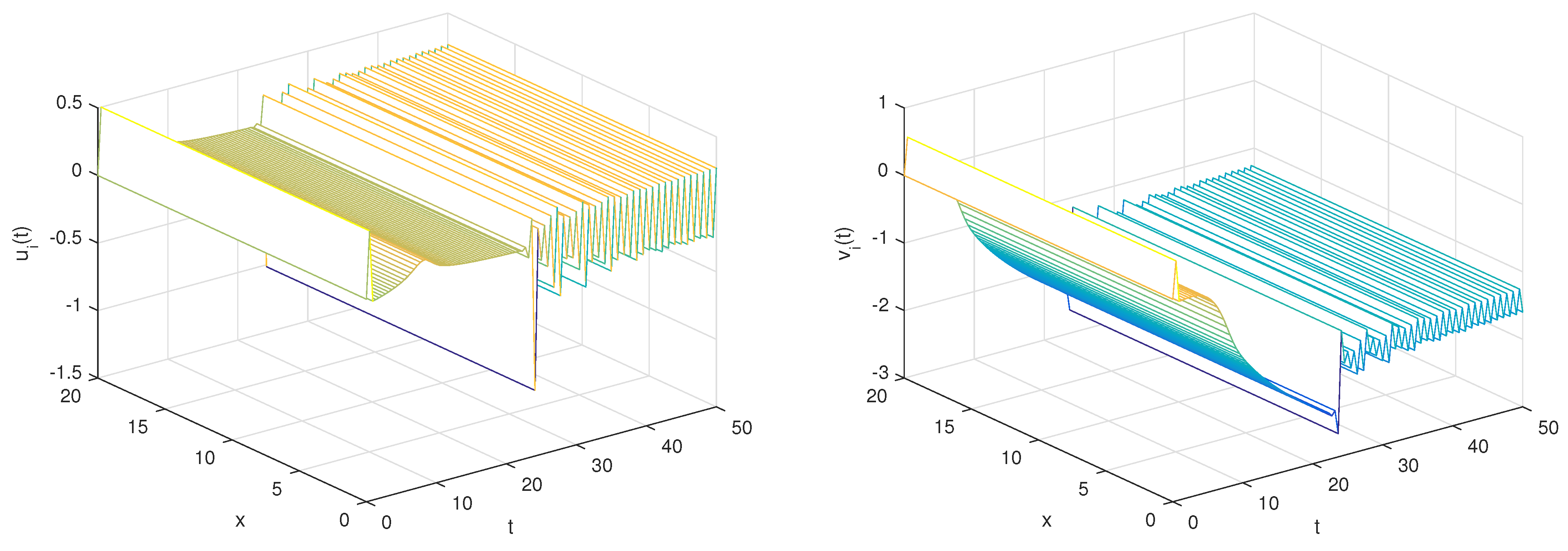
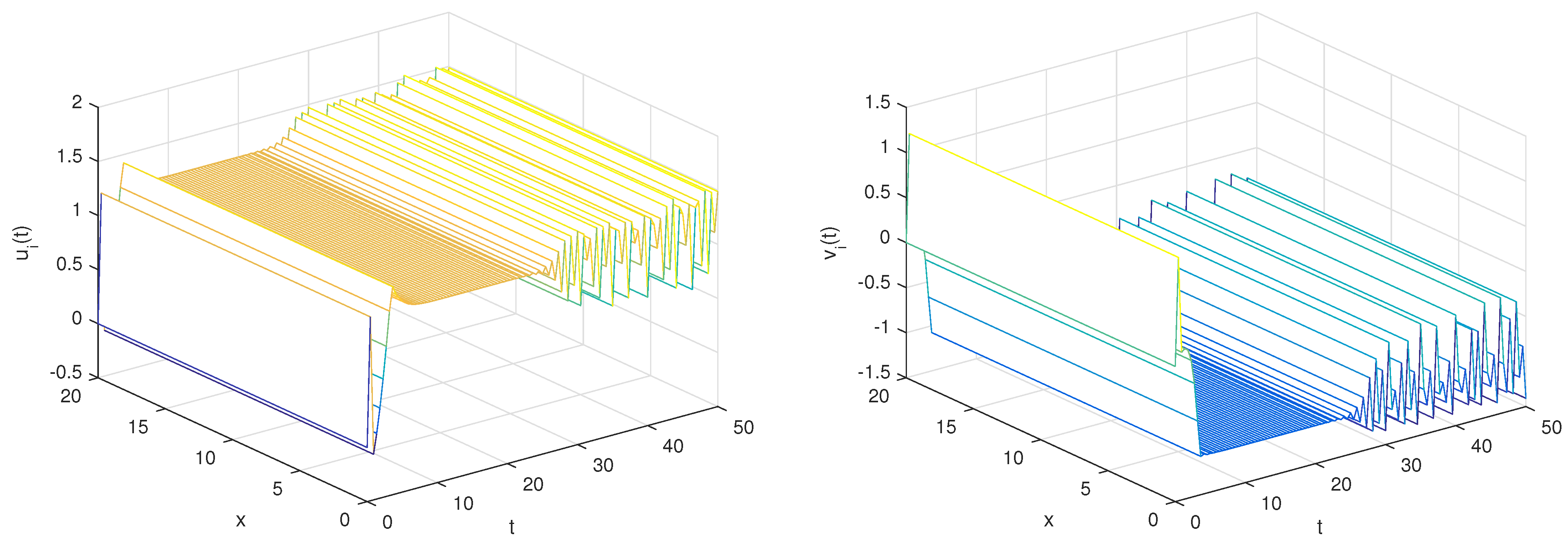
With the set of parameters,

$$(d_1,d_2,\mathfrak{a},\mathfrak{b})=(0.01,3,2.1,2),N=100,\hslash =0.1\xi =0.1,t\in [0,100],\kappa \in [0,20]$$

(29)

and the initial conditions

$$\left\{\begin{array}{c}({\mathfrak{H}}_1\left({\kappa }_i\right),{\mathfrak{H}}_2\left({\kappa }_i\right))=(2+cos\left(3\pi {\kappa }_i\right),3+cos\left(\pi {\kappa }_i\right)),\hfill \\ ({\mathfrak{G}}_1\left({\kappa }_i\right),{\mathfrak{G}}_2\left({\kappa }_i\right))=(5+cos\left(\pi {\kappa }_i\right),4+cos\left(\pi {\kappa }_i\right)).\hfill \end{array}\right.$$

(30)

To commence, the conditions stipulated in Theorem 3 are met, ensuring the applicability of the following linear controllers for governing the discrete fractional reaction–diffusion master–slave systems.

$$L=\left(\begin{array}{c}0.10\\ 00.7\end{array}\right).$$

(31)

By employing the given parameters, it becomes evident from Figure 1 and Figure 2 that the numerical solutions of the master–slave system exhibit a pronounced state of complete synchronization. Furthermore, Figure 3 portrays the error solution, underscoring its distinct trajectory toward asymptotic convergence to zero.

Case 2. 

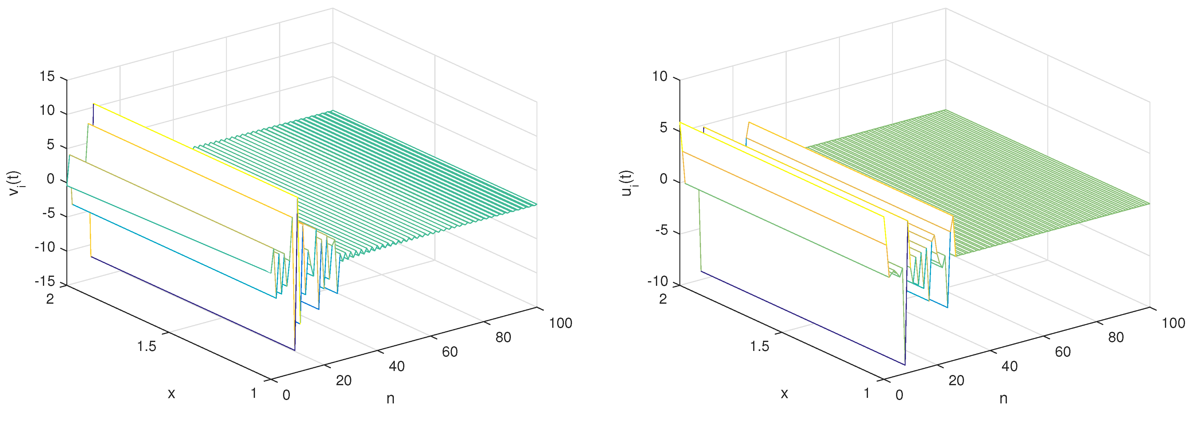
With the set of parameters

$$N=110,(d_1,d_2,\mathfrak{a},\mathfrak{b})=(1,1.5,2,0.5),\hslash =0.4,\xi =0.6t\in [0,100],x\in [0,20],$$

(32)

and the initial conditions

$$\left\{\begin{array}{c}({\mathfrak{H}}_1\left({\kappa }_i\right),{\mathfrak{H}}_2\left({\kappa }_i\right))=(3.5+cos\left(0.4\pi {\kappa }_i\right),3+cos\left(0.7\pi {\kappa }_i\right)),\hfill \\ ({\mathfrak{G}}_1\left({\kappa }_i\right),{\mathfrak{G}}_2\left({\kappa }_i\right))=(0.1+cos\left(\pi {\kappa }_i\right),0.5+cos\left(\pi {\kappa }_i\right)).\hfill \end{array}\right.$$

(33)

according to the guidelines provided in Theorem 2, the presence of a control matrix D facilitates the attainment of complete synchronization between the systems (26) and (27). The selection of matrix D can be made as follows:

$$D=\left(\begin{array}{c}20\\ 01.5\end{array}\right),$$

(34)

Hence, systems (26) and (27) exhibit complete global synchronization, as illustrated in Figure 4 and Figure 5. Additionally, the temporal progression of the error system states, denoted as $e_{1i}$ and $e_{2i}$, is visualized in Figure 6.

6. Conclusions

This paper delves into the exploration of the discrete counterpart of the model of fractional reaction–diffusion. In cases where the fractional order equates to one, the proposed system unveils itself as a discrete entity through the application of the forward difference schema. Simultaneously, the synchronization behavior within the scrutinized discrete master–slave systems undergoes investigation, with results aligning cohesively with those obtained from their continuous counterparts. This discernment underscores the capacity of a discrete system, structured upon an L1 finite difference scheme and a second-order central difference scheme, to retain the hallmarks of a continuous system, encompassing traits like positivity, boundedness, and synchronization dynamics facilitated by linear control laws and the Lyapunov functional. Ultimately, numerical simulations aptly showcase the efficacy and versatility of the proposed approach.

References

- Britton, N.F. Reaction–diffusion Equations and Their Applications to Biology; Academic Press: Cambridge, MA, USA, 1986. [Google Scholar]
- Song, Y.; Zhang, T.; Peng, Y. Turing–Hopf bifurcation in the reaction–diffusion equations and its applications. Commun. Nonlinear Sci. Numer. Simul. 2016, 33, 229–258. [Google Scholar] [CrossRef]
- Zhong, C.K.; Yang, M.H.; Sun, C.Y. The existence of global attractors for the norm-to-weak continuous semigroup and application to the nonlinear reaction–diffusion equations. J. Differ. Eq. 2006, 223, 367–399. [Google Scholar] [CrossRef]
- Kuttler, C. Reaction–diffusion equations and their application on bacterial communication. In Handbook of Statistics; Elsevier: Amsterdam, The Netherlands, 2017; pp. 55–91. [Google Scholar]
- Lam, K.Y.; Lou, Y. Introduction to Reaction–Diffusion Equations: Theory and Applications to Spatial Ecology and Evolutionary Biology; Springer Nature: Berlin/Heidelberg, Germany, 2022. [Google Scholar]
- Cosner, C. Reaction–diffusion equations and ecological modeling. In Tutorials in Mathematical Biosciences IV: Evolution and Ecology; Springer: Berlin/Heidelberg, Germany, 2008; pp. 77–115. [Google Scholar]
- Henry, B.I.; Wearne, S.L. Fractional reaction–diffusion. Phys. A Stat. Mech. Its Appl. 2000, 276, 448–455. [Google Scholar] [CrossRef]
- Seki, K.; Wojcik, M.; Tachiya, M. Fractional reaction–diffusion equation. J. Chem. Phys. 2003, 119, 2165–2170. [Google Scholar] [CrossRef]
- Gafiychuk, V.V.; Datsko, B.Y. Pattern formation in a fractional reaction–diffusion system. Phys. A Stat. Mech. Its Appl. 2006, 365, 300–306. [Google Scholar] [CrossRef]
- Saxena, R.K.; Mathai, A.M.; Haubold, H.J. Solution of generalized fractional reaction–diffusion equations. Astrophys. Space Sci. 2006, 305, 305–313. [Google Scholar] [CrossRef]
- Baeumer, B.; Kovács, M.; Meerschaert, M.M. Numerical solutions for fractional reaction–diffusion equations. Comput. Math. Appl. 2008, 55, 2212–2226. [Google Scholar] [CrossRef]
- Chen, L.; Qu, J.; Chai, Y.; Wu, R.; Qi, G. Synchronization of a class of fractional-order chaotic neural networks. Entropy 2013, 15, 3265–3276. [Google Scholar] [CrossRef]
- Ostalczyk, P. Discrete Fractional Calculus: Applications in Control and Image Processing; World Scientific: Singapore, 2015. [Google Scholar]
- Atici, F.M.; Uyanik, M. Analysis of discrete fractional operators. Appl. Anal. Discret. Math. 2015, 139–149. [Google Scholar] [CrossRef]
- Abdeljawad, T.; Banerjee, S.; Wu, G.C. Discrete tempered fractional calculus for new chaotic systems with short memory and image encryption. Optik 2020, 218, 163698. [Google Scholar] [CrossRef]
- Aticıi, F.M.; Sengul, S. Modeling with fractional difference equations. J. Math. Anal. Appl. 2010, 369, 1–9. [Google Scholar] [CrossRef]
- Algehyne, E.A.; Ibrahim, M. Fractal-fractional order mathematical vaccine model of COVID-19 under non-singular kernel. Chaos Solit. Fract. 2021, 150, 111150. [Google Scholar] [CrossRef] [PubMed]
- Saadeh, R.; Abbes, A.; Al-Husban, A.; Ouannas, A.; Grassi, G. The Fractional Discrete Predator–Prey Model: Chaos, Control and Synchronization. Fractal Fract. 2023, 7, 120. [Google Scholar] [CrossRef]
- Tuan, N.H.; Baleanu, D.; Thach, T.N.; O’Regan, D.; Can, N.H. Final value problem for nonlinear time fractional reaction–diffusion equation with discrete data. J. Comput. Appl. Math. 2020, 376, 112883. [Google Scholar] [CrossRef]
- Chen, H.; Lü, S.; Chen, W. Finite difference/spectral approximations for the distributed order time fractional reaction–diffusion equation on an unbounded domain. J. Comput. Phys. 2016, 315, 84–97. [Google Scholar] [CrossRef]
- Han, C.; Wang, Y.; Li, Z. Novel patterns in a class of fractional reaction–diffusion models with the Riesz fractional derivative. Math. Comput. Simul. 2022, 202, 149–163. [Google Scholar]
- Liu, F.; Turner, I.; Anh, V.; Yang, Q.; Burrage, K. A numerical method for the fractional Fitzhugh-Nagumo monodomain model. Anziam J. 2012, 54, C608–C629. [Google Scholar] [CrossRef]
- Majidabad, S.S.; Shandiz, H.T.; Hajizadeh, A. Decentralized sliding mode control of fractional-order large-scale nonlinear systems. Nonlinear Dyn. 2014, 77, 119–134. [Google Scholar] [CrossRef]
- Alsayyed, O.; Hioual, A.; Gharib, G.M.; Abualhomos, M.; Al-Tarawneh, H.; Alsauodi, M.S.; Abu-Alkishik, N.; Al-Husban, A.; Ouannas, A. On Stability of a Fractional Discrete Reaction–Diffusion Epidemic Model. Fractal Fract. 2023, 7, 729. [Google Scholar] [CrossRef]
- Kao, Y.; Cao, Y.; Chen, Y. Projective Synchronization for Uncertain Fractional reaction–diffusion Systems via Adaptive Sliding Mode Control Based on Finite-Time Scheme. IEEE Trans. Neural Netw. Learn. Syst. 2023. [Google Scholar] [CrossRef]
- Mesdoui, F.; Shawagfeh, N.; Ouannas, A. Global synchronization of fractional-order and integer-order N component reaction diffusion systems: Application to biochemical models. Math. Methods Appl. Sci. 2021, 44, 1003–1012. [Google Scholar] [CrossRef]
- Nicollin, X.; Olivero, A.; Sifakis, J.; Yovine, S. An Approach to the Description and Analysis of Hybrid Systems; International Hybrid Systems Workshop; Springer: Berlin/Heidelberg, Germany, 1991. [Google Scholar]
- Ouannas, A.; Wang, X.; Pham, V.T.; Grassi, G.; Huynh, V.V. Synchronization results for a class of fractional-order spatiotemporal partial differential systems based on fractional Lyapunov approach. Bound. Value Probl. 2019, 2019, 74. [Google Scholar] [CrossRef]
- Wu, G.C.; Baleanu, D. Chaos synchronization of the discrete fractional logistic map. Signal Process. 2014, 102, 96–99. [Google Scholar] [CrossRef]
- Zhou, T.; Li, C. Synchronization in fractional-order differential systems. Phys. D Nonlinear Phenom. 2005, 212, 111–125. [Google Scholar] [CrossRef]
- Yan, W.; Ding, Q. A new matrix projective synchronization of fractional-order discrete-time systems and its application in secure communication. IEEE Access 2020, 8, 147451–147458. [Google Scholar] [CrossRef]
- Abu Falahah, I.; Hioual, A.; Al-Qadri, M.O.; AL-Khassawneh, Y.A.; Al-Husban, A.; Hamadneh, T.; Ouannas, A. Synchronization of Fractional Partial Difference Equations via Linear Methods. Axioms 2023, 12, 728. [Google Scholar] [CrossRef]
- Wu, G.C.; Baleanu, D.; Zeng, S.D.; Deng, Z.G. Discrete fractional diffusion equation. Nonlinear Dyn. 2015, 80, 281–286. [Google Scholar] [CrossRef]
- Wu, G.C.; Baleanu, D.; Xie, H.P.; Zeng, S.D. Discrete fractional diffusion equation of chaotic order. Int. J. Bifurc. Chaos 2016, 26, 1650013. [Google Scholar] [CrossRef]
- Kelley, W.G.; Peterson, A.C. Difference Equations: An Introduction with Applications; Academic Press: Cambridge, MA, USA, 2001. [Google Scholar]
- Baleanu, D.; Wu, G.C.; Bai, Y.R.; Chen, F.L. Stability analysis of Caputo–like discrete fractional systems. Commun. Nonlinear Sci. Numer. Simul. 2017, 48, 520–530. [Google Scholar] [CrossRef]
- Hioual, A.; Ouannas, A.; Oussaeif, T.E.; Grassi, G.; Batiha, I.M.; Momani, S. On variable-order fractional discrete neural networks: Solvability and stability. Fractal Fract. 2022, 6, 119. [Google Scholar] [CrossRef]
- Elaydi, S. An Introduction to Difference Equations; Springer: San Antonio, TX, USA, 2015. [Google Scholar]
- Ahmed, N.; Ss, T.; Imran, M.; Rafiq, M.; Rehman, M.A.; Younis, M. Numerical analysis of auto-catalytic glycolysis model. AIP Adv. 2019, 9, 085213. [Google Scholar] [CrossRef]
- Al Noufaey, K.S. Stability analysis for Selkov-Schnakenberg reaction–diffusion system. Open Math. 2021, 19, 46–62. [Google Scholar] [CrossRef]
Disclaimer/Publisher’s Note: The statements, opinions and data contained in all publications are solely those of the individual author(s) and contributor(s) and not of MDPI and/or the editor(s). MDPI and/or the editor(s) disclaim responsibility for any injury to people or property resulting from any ideas, methods, instructions or products referred to in the content. |
© 2023 by the authors. Licensee MDPI, Basel, Switzerland. This article is an open access article distributed under the terms and conditions of the Creative Commons Attribution (CC BY) license (https://creativecommons.org/licenses/by/4.0/).
Share and Cite
Hamadneh, T.; Hioual, A.; Saadeh, R.; Abdoon, M.A.; Almutairi, D.K.; Khalid, T.A.; Ouannas, A. General Methods to Synchronize Fractional Discrete Reaction–Diffusion Systems Applied to the Glycolysis Model. Fractal Fract. 2023, 7, 828. https://doi.org/10.3390/fractalfract7110828
Hamadneh T, Hioual A, Saadeh R, Abdoon MA, Almutairi DK, Khalid TA, Ouannas A. General Methods to Synchronize Fractional Discrete Reaction–Diffusion Systems Applied to the Glycolysis Model. Fractal and Fractional. 2023; 7(11):828. https://doi.org/10.3390/fractalfract7110828
Chicago/Turabian StyleHamadneh, Tareq, Amel Hioual, Rania Saadeh, Mohamed A. Abdoon, Dalal Khalid Almutairi, Thwiba A. Khalid, and Adel Ouannas. 2023. "General Methods to Synchronize Fractional Discrete Reaction–Diffusion Systems Applied to the Glycolysis Model" Fractal and Fractional 7, no. 11: 828. https://doi.org/10.3390/fractalfract7110828
APA StyleHamadneh, T., Hioual, A., Saadeh, R., Abdoon, M. A., Almutairi, D. K., Khalid, T. A., & Ouannas, A. (2023). General Methods to Synchronize Fractional Discrete Reaction–Diffusion Systems Applied to the Glycolysis Model. Fractal and Fractional, 7(11), 828. https://doi.org/10.3390/fractalfract7110828