Fractional-Order Modeling of Piezoelectric Actuators with Coupled Hysteresis and Creep Effects

Abstract

A novel fractional-order model, incorporating coupled hysteresis and creep effects, is proposed for typical piezoelectric actuators in this study. Throughout the actuation process, various nonlinear behaviors such as piezoelectric hysteresis, non-local memory, peak transition, and creep nonlinearity are accurately characterized by the model. Offering a simpler structure and superior tracking performance compared to conventional models, the proposed fractional-order model parameters are identified using a method that integrates actuator dynamics and employs the particle swarm optimization algorithm. Experimental validation on a piezoelectric actuation platform confirms the model’s superior accuracy and simplified structure, contributing to a deeper understanding of piezoelectric actuation mechanisms and providing an efficient modeling tool for enhanced system performance.

1. Introduction

Piezoelectric actuators (PEAs) are extensively utilized in micro-vibration control and isolation [1,2,3], high-precision positioning [4,5], and manufacturing equipment [6,7]. Their exceptional characteristics, including substantial output, high resonance frequency, precision, and compact size, render them indispensable. Notable applications include a three-degree-of-freedom (3-DOF) micro-vibration isolation platform, a piezo stack energy harvester [8], nanopositioning stages [9], and atomic force microscopy [10], all leveraging PEAs. Unfortunately, the inherent hysteresis and creep nonlinearities significantly impede their operational accuracy [11]. The hysteresis effect alone can induce a substantial maximum displacement error of 10–15% in the open loop [12]. Additionally, the creep effect severely compromises open-loop accuracy at low frequencies [13]. To enhance PEA positioning accuracy, a thorough investigation into the coupled effects of hysteresis and creep is imperative, along with the exploration of strategies to overcome these nonlinear limitations.

Modeling and compensating for the nonlinear characteristics of PEAs is considered the most effective method; hence, accurate nonlinear modeling is crucial [14]. Hysteresis modeling methods are broadly categorized into two types: physics-based models [15,16] and phenomenon-based models. Accurately identifying parameters for physics-based models is challenging [17]. Phenomenon-based models describe hysteresis by correlating input voltage with output displacement, encompassing models such as the Bouc–Wen model [18,19], Prandtl–Ishlinskii model [20,21], Preisach model [22], etc. These models can be seamlessly integrated with complex algorithms for identification [23,24]. Among them, the static Bouc–Wen model stands out as a popular and effective choice for representing lag effects independently of the rate. However, both the existing Bouc–Wen model and its enhancements encounter challenges related to complex model information and the precise acquisition of parameters. Therefore, this paper introduces a simplified phenomenon-based fractional hysteresis model to portray rate-independent hysteresis.

Creep, as another nonlinear behavior of PEAs, manifests as a gradual drift in displacement following abrupt changes in input voltage, significantly impacting absolute positioning [25]. The current literature details two primary modeling methods for creep: a logarithmic model [26] and a spring-damper model [27,28]. The former establishes a linear relationship between output displacement and logarithmic time [29,30]. Meanwhile, the latter, although effective, poses challenges in parameter identification due to its complexity [31]. Fractional-order creep dynamics, introduced to address these challenges, leverage a physics-based fractional-order Maxwell resistive capacitor approach [32]. Despite the effectiveness of the spring-damper method in experiments, existing graded creep models oversimplify nonlinearity induced by frequency changes in the low-frequency range. To tackle this, the paper presents a novel parameter identification method utilizing the dynamic system equation of PEAs, aiming to enhance the accuracy of graded creep models.

In the practical actuation process of PEAs, various features come into play, including the two nonlinear behaviors mentioned earlier. These features are intertwined and exert mutual influence throughout PEA actuation. To refine the accuracy of the actuation model for piezoelectric ceramic actuators, researchers have delved into studying the coupling model [9,33]. Addressing the intricacies arising from hysteresis and linear dynamics coupling, a novel decoupling identification method is introduced. This method, grounded in the assumption that the hysteresis part operates independently of the rate, employs a sinusoidal input with low frequency and wide amplitude to establish the Bouc–Wen model. Subsequently, a harmonic linearization method is utilized to deduce the true input to the linear part, effectively decoupling hysteresis for accurate linear dynamics identification. To further refine the modeling accuracy of piezoelectric actuators, [34] suggests adopting a fractional-order coupled model. Building on the contributions of prior researchers, this paper introduces a novel fractional-order hysteresis and creep model. This model seeks to elevate the accuracy of describing hysteresis and creep phenomena, along with their coupled behaviors in PEAs.

The introduced fractional-order model here is implemented based on the mathematical tools of fractional calculus. The origin of fractional calculus can be traced back to the period when Newton and Leibniz first established traditional calculus. Noteworthy scholars, including the French mathematician Liouville in 1834, the German mathematician Riemann in 1847, the Czech mathematician Grunwald in 1867, and the Russian mathematician Letnikov in 1868, proposed meaningful definitions for fractional calculus. Subsequently, Liouville and Riemann’s definitions led to the Riemann–Liouville (R-L) definition [35], while Grunwald and Letnikov’s definitions were integrated into the Grunwald–Letnikov (G-L) definition [36]. Both of these definitions are suitable for describing fractional calculus problems involving functions with zero initial values in applications [37]. This includes the use of the R-L-defined fractional differential diffusion equation to depict the slow relaxation processes in complex systems such as polymers and even biological tissues [38]. The application of the G-L-defined two-dimensional isotropic gradient operator mask is employed to enhance image texture information [39], and the application based on the G-L definition aims to minimize the contribution of natural environmental noise components [40]. Additionally, for cases with non-zero initial values, the definition introduced by the Italian mathematician Caputo in 1967 is very useful; further elaboration will be provided in subsequent sections. Thus, it can be observed that fractional calculus provides a more flexible modeling approach, allowing for a better capture of dynamic behavior in non-integer dimensions. For complex systems, especially those with memory and non-local characteristics, fractional calculus models have the ability to more effectively capture the long-term dynamic properties of the system than the traditional integer order models.

Therefore, building on the advantages of fractional calculus models, this paper introduces a six-parameter fractional-order hysteresis and creep-coupled model designed to accurately describe piezoelectric effects. The main text outlines an identification approach that harnesses the inherent properties of the model, demonstrated through the accurate implementation of a particle swarm algorithm. Comprehensive simulations and experimental studies are showcased to authenticate the effectiveness of the proposed fractional-order model and the corresponding parameter identification.

The main contributions of this paper are summarized as follows:

• A novel fractional-order hysteresis model with five parameters, including linear and nonlinear components, is proposed to capture the rate-independent hysteresis effect and the main characteristics of PEAs.
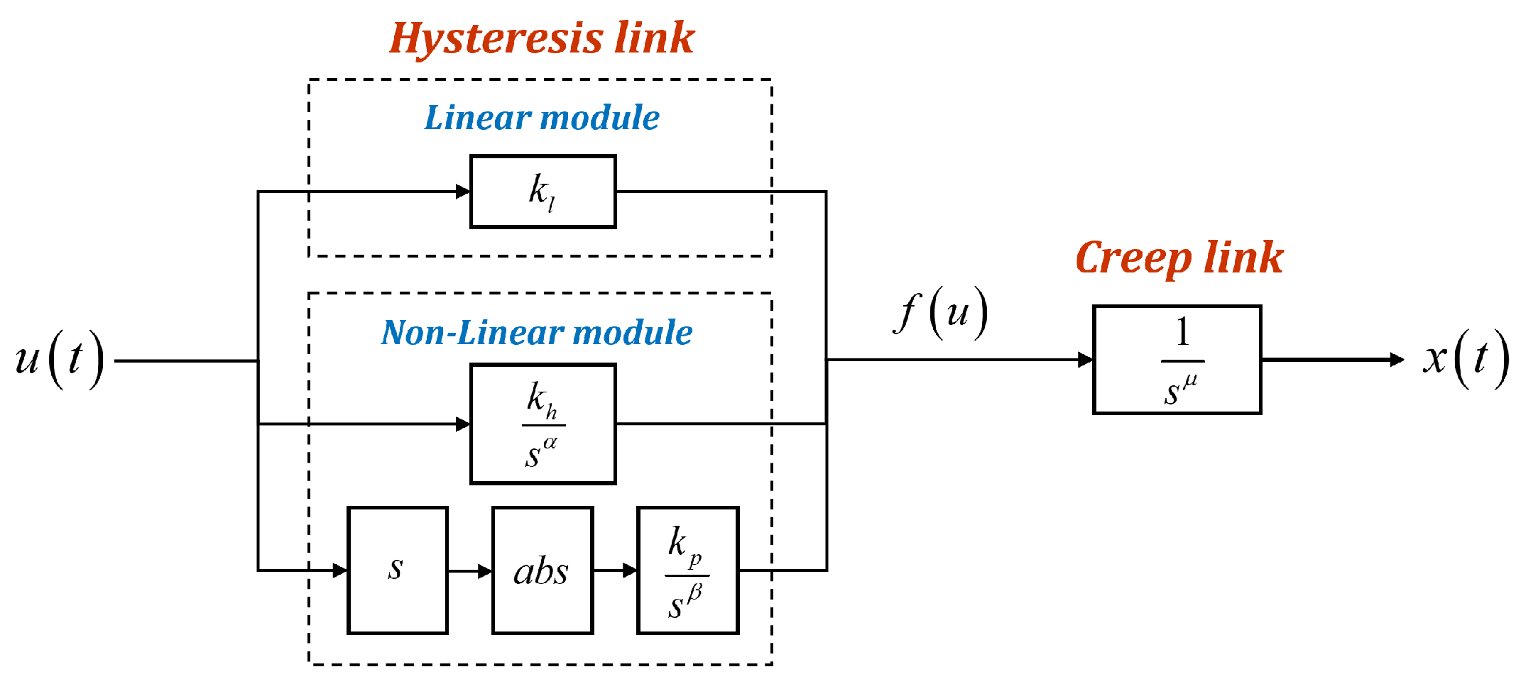
• Then, it is proposed to combine the fractional-order creep model with the dynamic model of PEAs and identify the creep parameters and dynamic parameters simultaneously, so as to eliminate dynamic interference and improve the identification accuracy of the creep module.
• Finally, we affirm the verification of the enhanced accuracy achieved by the proposed model in capturing the nonlinear coupled effects of hysteresis and creep, validated through experimental evidence.

This article is organized as follows. Section 2 presents a fractional-order hysteresis and creep modeling approach and the coupled model. Section 3 investigates the properties of the proposed fractional-order model. Section 4 presents the fractional-order model parameter identification method and experimental verification results. Finally, Section 5 gives the conclusion of the paper.

2. Fractional-Order Modeling of Hysteresis and Creep for PEAs

In this study, we introduce a fractional-order hysteresis and creep-coupled model for PEAs. The proposed fractional-order hysteresis (FOH) model captures piezo hysteresis, and fractional-order drift dynamic characterize the creep phenomenon. Notably, this coupled model achieves accurate representation with a minimal set of only six parameters.

2.1. Fractional Calculus Definition and Model Theory

In mathematics, fractional calculus is a branch of mathematical analysis that investigates the potential applications of real powers of a differentiation operator $D=\frac{d}{dx}$ and an integration operator J. Herein, a unified operator ${}_{t_0}{D}_t^{\alpha }$ for fractional-order differentiation and integration is introduced and widely applied in the establishment of the model presented in this paper. Its definition [41] is as follows:

$${}_{t0}{D}_t^{\alpha }f\left(t\right)=\left\{\begin{array}{c}\frac{d^{\alpha }}{d{t}^{\alpha }}f\left(t\right),\alpha >0\hfill \\ f\left(t\right),\alpha =0\hfill \\ {\int }_{t_0}^{t}f\left(\tau \right)d{\tau }^{-\alpha },\alpha <0\hfill \end{array}\right.$$

(1)

where $\alpha$ is confined to real numbers, with t representing the independent variable and $t_0$ as its lower bound.

When selecting the calculus principles to implement operators in mathematical models, choosing a proper definition of fractional calculus becomes a challenge. In the definitions of fractional calculus, both G-L and R-L have difficulties in describing differential equations when non-zero initial conditions are present. Therefore, in the study of non-zero initial condition systems, such as the voltage–displacement relationship in piezoelectric materials explored in this paper, it is necessary to introduce the Caputo definition, which allows for the utilization of initial values of classical integer-order derivatives with known physical interpretations [42,43]:

$$\begin{array}{cc}\hfill {}_{t_0}^C{D}_t^{\alpha }y\left(t\right)& ={}_0^C{D}_t^{\alpha }y\left(t\right)=\frac{d^{\alpha }y\left(t\right)}{d{t}^{\alpha }}\hfill \\ \hfill & =\frac{1}{\Gamma \left(m-\alpha \right)}{\int }_0^t\frac{y^{\left(m\right)}\left(\tau \right)}{{\left(t-\tau \right)}^{\alpha +1-m}}d\tau \hfill \end{array}$$

(2)

In the given expression, m is an integer such that $m-1<\alpha <m$, where $\alpha$ represents the order of the fractional derivative. The term $y^{\left(m\right)}\left(\tau \right)$ denotes the mth derivative of $y\left(\tau \right)$, and $\Gamma \left(m-\alpha \right)$ represents the Gamma function evaluated at the independent variable $m-\alpha$.

In the more common scenario of engineering implementation, a band-limit implementation is required to compute ${\left(\frac{1}{s}\right)}^{\alpha }$ (where $\alpha$ is a fraction), and the frequency range is stipulated as $\left({\omega }_b,{\omega }_h\right)$. By employing the Oustaloup recursive algorithm [44], the approximate transfer function as follows:

$$G\left(s\right)=K\prod _{i=-N}^N\frac{s+\omega {}_i^{\prime }}{s+{\omega }_i}$$

(3)

where K, $w{}_i^{\prime }$, and $w_i$ denote the gain, zeros and poles, respectively, of the approximate transfer function $G\left(s\right)$. The parameter N signifies the approximate order. The computation of zeros, poles, and gain is performed by

$$\omega {}_i^{\prime }={\omega }_b{\left(\frac{{\omega }_h}{{\omega }_b}\right)}^{\frac{k+N+\frac{1}{2}\left(1+\mu \right)}{2N+1}}$$

(4)

$${\omega }_i={\omega }_b{\left(\frac{{\omega }_h}{{\omega }_b}\right)}^{\frac{k+N+\frac{1}{2}\left(1-\mu \right)}{2N+1}}$$

(5)

$$K={\left(\frac{{\omega }_h}{{\omega }_b}\right)}^{\frac{\mu }{2}}\prod _{i=-N}^N\frac{{\omega }_i}{\omega {}_i^{\prime }}$$

(6)

when s approaches infinity, the approximate transfer function $G\left(s\right)$ converges to K. Conversely, as s tends to zero, $G\left(s\right)$ approaches ${\left(\frac{{\omega }_h}{{\omega }_b}\right)}^{\frac{\mu }{2}}$.

2.2. Features of the Fractional-Order Operator

As introduced in the opening section, the phenomenological modeling approach treats the internal structure of the piezoelectric ceramic system as a black box, whether entirely or partially unobservable. It abstains from delving into the physical properties of the system’s internal structure and materials, concentrating solely on the external input–output characteristics.

Based on such principles, we have conducted research on the input–output mapping relationships of classical fractional-order operators and captured some dynamic behaviors that align well with the hysteresis nonlinearity characteristics observed in the actuation process of piezoelectric ceramics. A classical fractional-order operator can be expressed as

$$G\left(s\right)=\frac{Y\left(s\right)}{X\left(s\right)}=\frac{k}{s^{\mu }}$$

(7)

where k represents the gain, and $\mu \in \left[-1,1\right]$ is the fractional order. Various combinations of parameters k and $\mu$ result in distinct input–output mappings of the fractional-order operator.

Through the use of these fractional-order operators in simulation, we capture some dynamic behaviors. The input to the fractional-order operator is a small bidirectional trajectory signal with local reversals, and the signal does not represent a specific physical meaning. Figure 1a and Figure 1b respectively show the time-domain signal of the output and the input–output hysteresis mapping relationship:

Figure 1a illustrates the time-domain lag of the output $y\left(t\right)$ of the fractional-order operator concerning the original bidirectional input signal $x\left(t\right)$ for various $\mu$ values ($\mu$ = 0.1, 0.3, 0.5). In Figure 1b, the characteristics of the hysteresis loop between input and output are more intuitively reflected. Different combinations of k and $\mu$ values configure such nonlinear relationships. This grants the fractional-order operator a substantial advantage in describing nonlinear behaviors. Based on this advantage, attempts are made to construct a fractional-order nonlinear model.

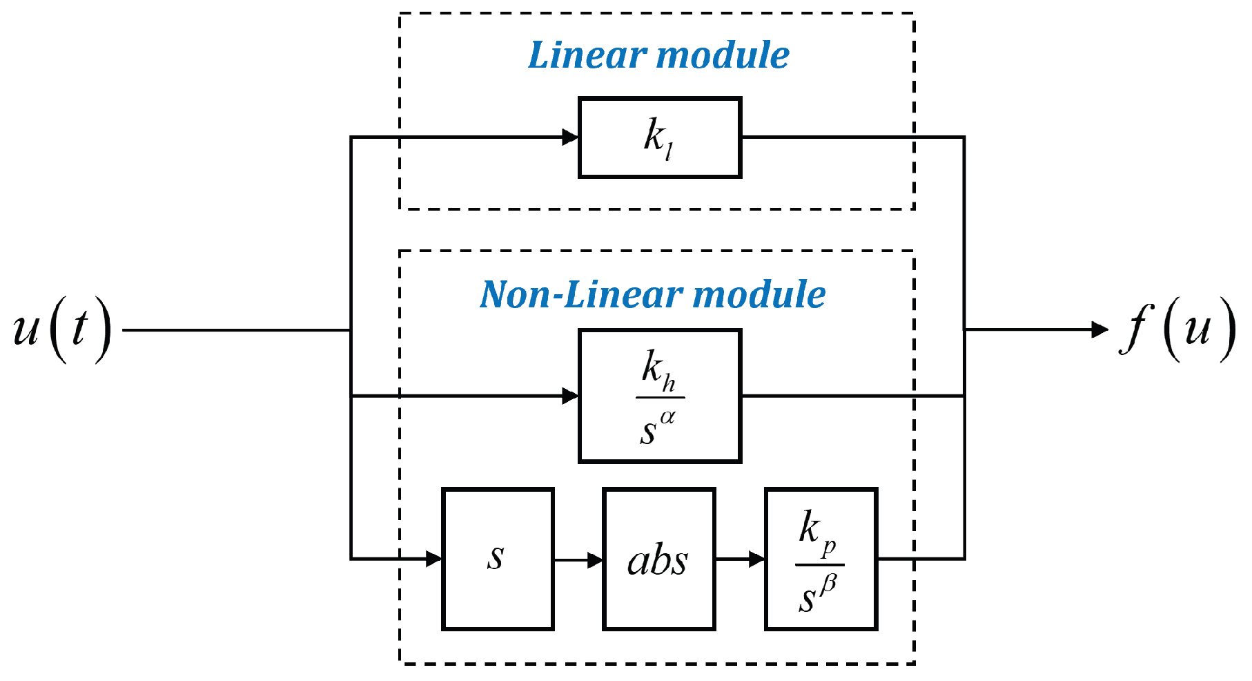
2.3. Fractional-Order Hysteresis Model

For an actual piezoelectric ceramic actuator system, Figure 2 illustrates the measured hysteresis curve of a PEA driven by a sinusoidal voltage signal with 1 Hz frequency and the input signal presented in Figure 3. The output displacement during the stable period is slightly different from that used in the initial period, attributed partly to loading oscillations and partly to the charge–discharge memory effect of the piezoelectric ceramic material.

In this study, when considering the line fitted by the least-squares method as the linear component, the hysteresis curve shown in Figure 2 can be decomposed into a linear displacement component and a hysteresis displacement component, as depicted in Figure 4 respectively. Observing Figure 4, it can be noted that the experimentally measured hysteresis curve can be viewed as the superposition of a linear component and a hysteresis component.

Therefore, in modeling the hysteresis effects of the PEA, the proposed fractional-order model is also divided into two parts, namely the linear module and the nonlinear module, to predict the linear and hysteresis components separately. The structure of the FOH model is shown in Figure 5.

The FOH model can be specifically divided into two parts, the linear component and the nonlinear component, expressed by Equation (8) and Equation (9), respectively. The linear component module is expressed by

$$f_l\left(u\right)=k_l·u\left(t\right)$$

(8)

where $u\left(t\right)$ is the input voltage, $k_l$ is the linear coefficient, and the model adjusts the linear coefficient to characterize the reference amplitude of the hysteresis curve under input voltage. Meanwhile, the specific content of the nonlinear module is given by

$$f_h\left(u\right)=k_h·D_t^{\alpha }u\left(t\right)+k_p·\left|\dot{u}\left(t\right)\right|D_t^{\beta }u\left(t\right)$$

(9)

where $D_t^{\alpha }u\left(t\right)$ and $D_t^{\beta }u\left(t\right)$ are two fractional-order operators in the nonlinear component module; $k_h$ and $k_p$ are their nonlinear coefficients, respectively; and $\left|\dot{u}\left(t\right)\right|$ is the absolute value of the first order derivative of the signal $u\left(t\right)$, which is mainly responsible for controlling the relative magnitude of the hysteresis when the input signal suddenly changes.

2.4. Review of the Fractional-Order Creep Model

Liu et al. introduced a fractional-order creep model to characterize the creep phenomenon in PEAs [34]. This model is derived from an analysis of the series model of the spring–damper system. By manipulating the order of the spring-damping system and adjusting model parameters, the transfer function of the model is formulated as

$$G_c\left(s\right)=k_c\prod _i\frac{s+z_i}{s+p_i}$$

(10)

where $k_c$, $z_i$, and $p_i$ denote the gain, zeros, and poles of the creep system transfer function, respectively.

Notably, Equations (3) and (10) share an identical form. As the frequency increases, the creep’s magnitude decreases, and the phase remains approximately constant, as illustrated in Figure 6. Here, the fractional-order creep system function can be expressed as

$$G_c\left(s\right)=k_c{\left(\frac{1}{s}\right)}^{\mu }$$

(11)

where $k_c$ and $\mu$ represent the gain and fractional power of the fractional-order creep dynamic model. The coefficient $k_c$ of this creep model is incorporated into the coupling hysteresis link, resulting in a fractional-order model that encapsulates the combined influences of hysteresis and creep behavior.

2.5. Fractional-Order Hysteresis and Creep-Coupled Model

In this section, based on the newly proposed FOH model and the just-reviewed fractional-order creep dynamic model, a novel hysteresis and creep-coupled model is proposed. Its cascade structure is shown in Figure 7.

The FOH model and fractional-order creep model are interconnected, and the input information is transmitted through the $f\left(u\right)$ obtained after the hysteresis process in the middle to predict the hysteresis behavior of the PEAs under repeated loading and the creep behavior under long-term loading. Two fractional-order models describing the most important nonlinear characteristics of piezoelectric actuation are coupled, with only six parameters and a compact structure. The coupled model can accurately predict the corresponding model displacement output $x\left(t\right)$ under the input signal $u\left(t\right)$. The following chapter investigates the characterization of the proposed models on the hysteresis and creep effects of PEAs.

3. Properties of the Proposed Models

In this section, we delve into the attributes of the FOH model and the fractional-order creep model. The examination of the FOH model involves subjecting it to a sine signal input, with subsequent analysis utilizing Bode diagrams and step response simulations. Concurrently, fractional-order creep modeling is scrutinized through a comprehensive study involving Bode diagrams and step response simulations. The proposed coupled model undergoes investigation employing variable–frequency sinusoidal input.

3.1. Properties of the FOH Model

The FOH model takes advantage of the hysteresis properties of the fractional-order operator, exhibiting the characteristic behavior of lagging behind changes in the input signal. The proposed hysteresis model shows the following characteristic behavior with sinusoidal input, which is consistent with the actual PEAs.

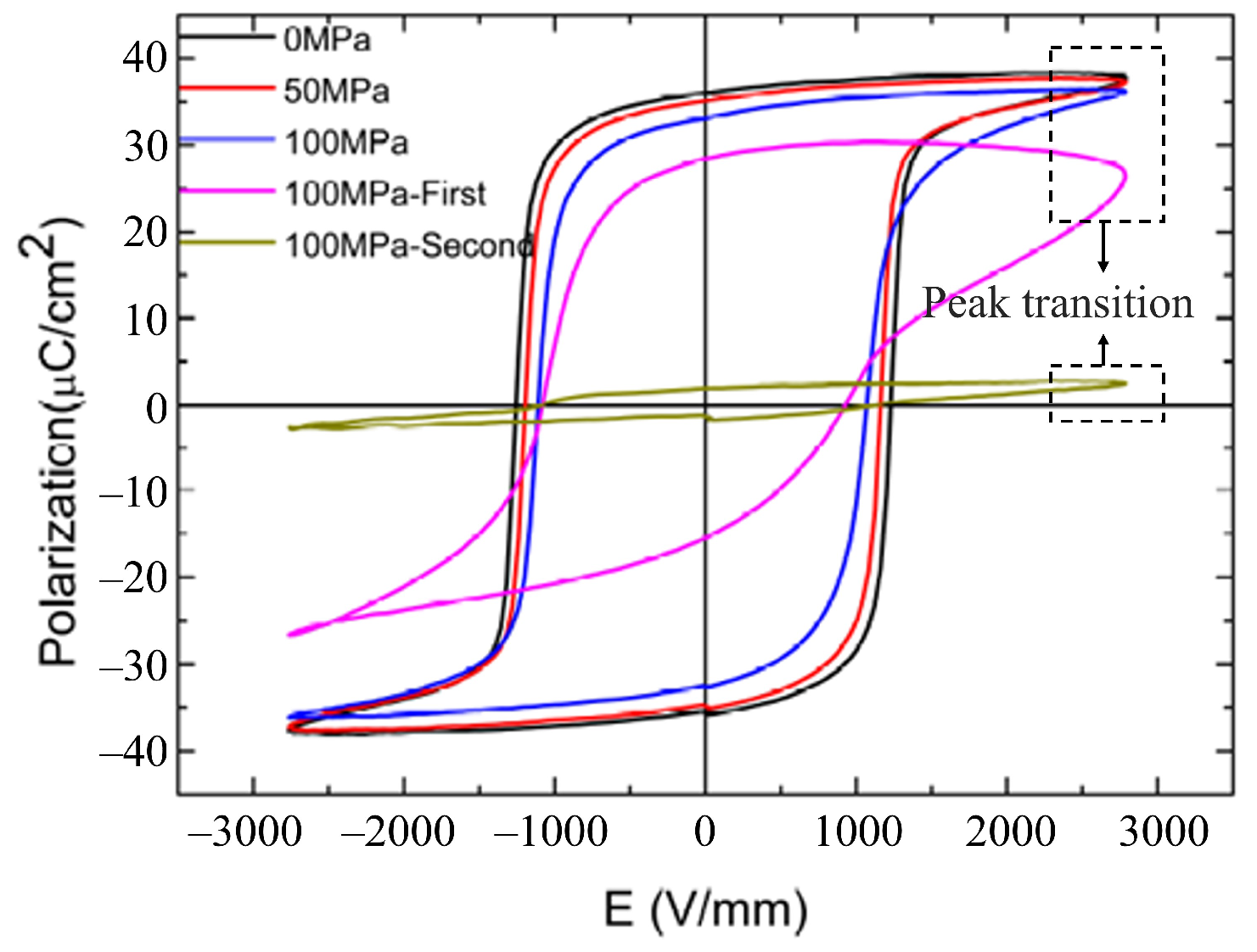
3.1.1. Peak Transition Behavior

Piezoelectric ceramics, as a type of polar dielectric material, undergo polarization or changes in polarization state under the influence of an electric field, transmitting the effect of the electric field in an inductive manner [45]. Polarization intensity, typically denoted as P, is the physical quantity describing the strength of polarization [46]. Within a volume element $\Delta V$ in piezoelectric ceramics, when there is no external electric field, no polarization or change in polarization occurs. At this point, the vector sum $\Sigma p$ of the dipole moments of all atoms (or molecules) within the volume element $\Delta V$ is zero. Under the action of an electric field, polarization occurs in piezoelectric ceramics, and the vector sum of the dipole moments within the volume element is nonzero.

From a microscopic perspective, there are three scenarios for the generation of polarization [47]: electronic displacement polarization, ionic displacement polarization, and orientational polarization (also known as directional polarization). From a macroscopic viewpoint, the repeated charging and discharging of piezoelectric materials leads to the process of domain reorientation [48], characterized by peak transition behavior caused by the reversal after reaching the peak of the input voltage, as shown in Figure 8. Although the model proposed in this paper is obtained by fitting internal parameters through a phenomenological modeling approach, the rational configuration of fractional-order operators can also capture the microscopic–macroscopic phenomena, including peak transition behavior.

In previous studies on modeling the nonlinear characteristics of piezoelectric materials, a large number of nonlinear hysteresis operators were often employed to describe the hysteresis properties [49]. However, little additional attention was given to the peak transition behavior. The nonlinear component of the model proposed in this work is based on a combination of a fractional-order operators and a deformed form of another fractional-order operator, achieving a good representation of the peak transition behavior. Figure 9 demonstrates that the nonlinear module of the FOH model provides a better representation of this characteristic compared to a single fractional-order operator.

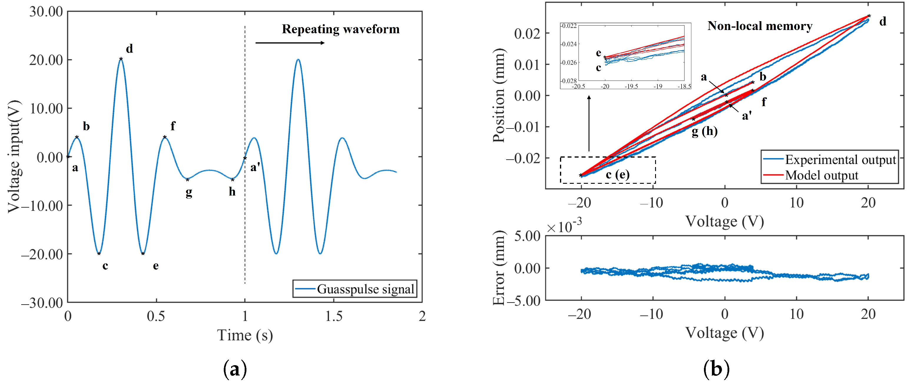
3.1.2. Piezo Lag and Non-Local Memory Effect

By applying an input signal, the PEA generates an inverse piezoelectric effect, achieving specific displacement to fulfill the corresponding driving purpose. During the reciprocating loading process of the input signal, the PEA exhibits a phenomenon where the displacement curves for increasing and decreasing voltage do not overlap, indicating a delay in the material’s response compared to the change in the cause. This phenomenon is known as piezo lag.

Simultaneously, in piezoelectric actuators, non-local memory refers to the internal changes in charge distribution that occur when an external electric field is applied, causing deformation of the material. Moreover, this evolution can be maintained for a certain period even after removing the electric field, forming a non-volatile information storage state. Consequently, the displacement output of the piezoelectric actuator is correlated with the previous-stage voltage input, providing a microscopic explanation for the principle behind macroscopic non-local memory.

From a system perspective, the output depends not only on the current input but also on the historical process of the input. This aspect is also in line with the characteristics of fractional calculus. In the simulation and experiments of the proposed model in this paper, the Gauss pulse waveform shown in Figure 10a (which has characteristics of quasi-periodicity, a prominent single peak, and symmetrical peaks on both sides) is input into the model system. Such a waveform allows for the control of equal amplitude inputs on both sides of the peaks for convenient comparison of output results. The results are then shown in Figure 10b.

To provide an intuitive correspondence between input and output, corresponding points are marked in Figure 10a,b. Notably, in Figure 10b, points c and e, as well as g and h, are very close but different, and only one position is marked for each pair. It can be observed that the large hysteresis loop in the $c-d-e$ segments of the model output exhibits the characteristics of piezo lag. Meanwhile, in segments $a-b-c$ and $e-f-g$, with equal input peak values, the displacement output is related to the historical inputs a and e, respectively, demonstrating different output values. This illustrates the dependence of the system output on the historical inputs for the same input, i.e., non-local memory. Despite the presence of errors between the model output and the experimental output, in terms of feature representation, this consistency in the experimental and simulated results in Figure 10 verifies the FOH model’s ability to predict and describe this phenomenon.

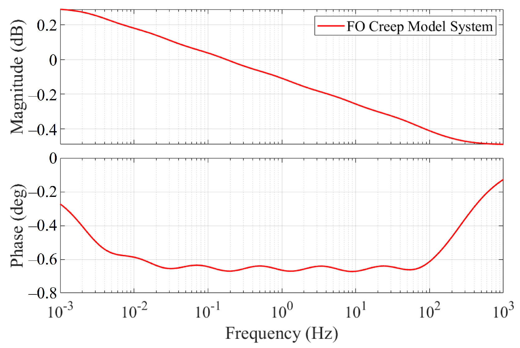
3.2. Properties of the Fractional-Order Creep Model

Model properties are assessed by observing the behavior of the fractional-order creep model in both time and frequency domains.

In the time domain, the model manifests a distinctive gradual drift phenomenon in its step response. This behavior is elucidated through the output curve illustrated in Figure 11, depicting the response generated by the model under a 100 V step excitation. For this illustrative scenario, specific parameter values are chosen, namely $k_c=0.0017$, $\mu =0.0072$, and a deliberate consideration of experimentally observed creep effects.

Turning to the frequency domain, the fractional-order creep model exhibits noteworthy features. With an increase in frequency, the phase of the model remains constant, accompanied by a consistent decrease in magnitude. Figure 12 presents the Bode diagram of the fractional-order model, bearing a resemblance to the Oustaloup implementation. The chosen frequency range for analysis is (0.01 Hz, 100 Hz). Remarkably, the phase–frequency curve of the proposed model assumes a distinct horizontal line shape, maintaining a constant phase of $-90 \mu \left(-0.648\right)$ deg. This alignment with the phase characteristics observed in the piezoelectric creep effect enhances the model’s significance in capturing and representing relevant physical phenomena.

3.3. Properties of the Coupled Model

Coupled models employ the cascade model to characterize hysteresis and creep effects, given their substantial impact on the accuracy of PEA applications. The subsequent analysis aims to assess the performance of the fractional-order creep- and fractional-order hysteresis-coupled models in response to low-frequency sine signal inputs with varying frequencies.

Figure 13 visually encapsulates the features of the coupled model. Notably, the hysteresis curves exhibit distortion owing to the frequency-dependent attenuation of the fractional-order creep magnitude. As depicted, the output displacement amplitude experiences a discernible reduction with the continuous increase in input signal frequency post the 1 Hz threshold. This observed phenomenon impeccably aligns with the amplitude–frequency characteristics of the creep model. The discernible decrease in output displacement amplitude as the input signal frequency rises beyond 1 Hz corroborates the consistent representation of creep effects by the coupled model. This noteworthy alignment substantiates the coupled model’s capacity not only to capture the hysteresis effect but also to faithfully represent the intricacies of the creep phenomenon.

In terms of the comprehensive representation of the model, the assessment of the fractional-order coupled model’s performance under low-frequency sine signal inputs reveals its aptitude for encapsulating both hysteresis and creep effects. This substantiates the model’s efficacy and suitability for applications in PEA systems.

4. Identification and Verification of the Fractional-Order Coupled Model

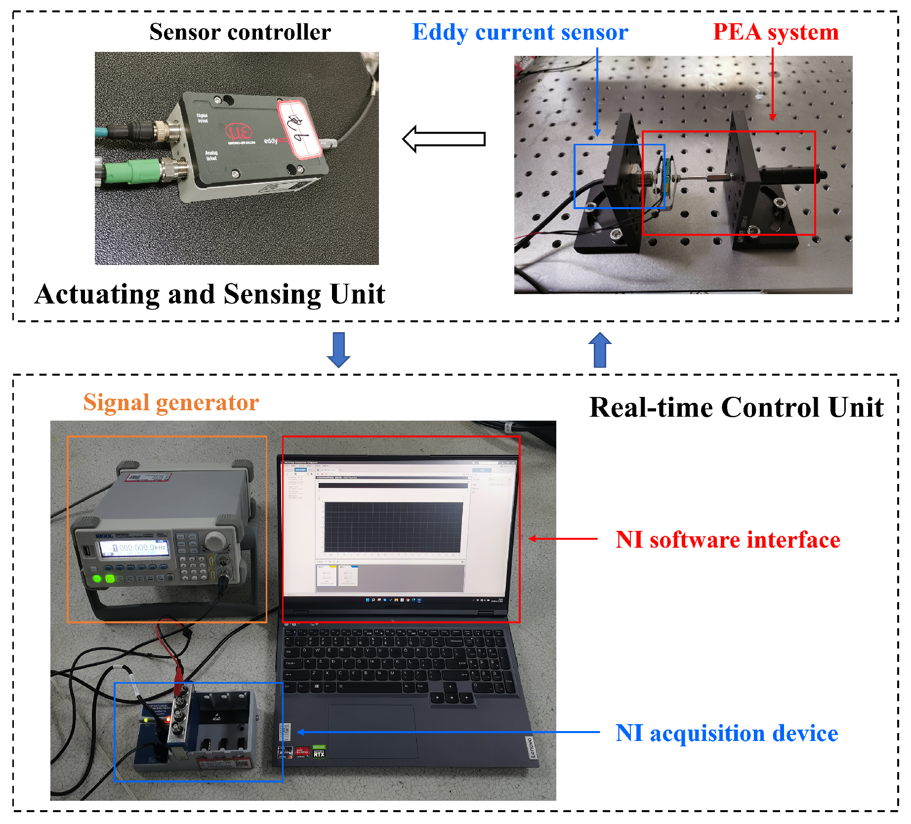
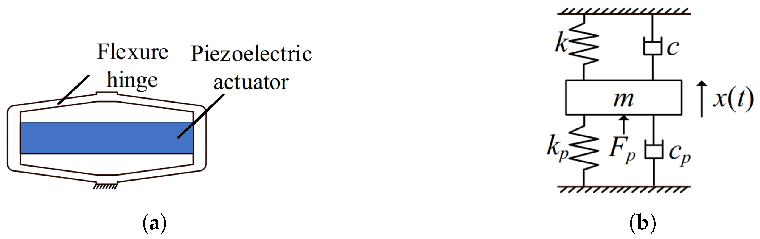
4.1. Experimental Setup

The experimental setup, as illustrated in Figure 14, involves a PEA with model P06.X200AK (nominal stroke: 0∼$120 \mathrm{V}$, nominal displacement: 160 μm $\pm 15\%$, Harbin Zhuanjing Technology Co., Ltd., Harbin, China). The PEA is driven by a voltage amplifier (model E53.C1K, capable of communication with the upper computer). Real-time measurement of its output displacement is conducted using an eddy current displacement sensor (eddyNCDT 3060, Mirco-epsilon Company, Ortenburg, Germany).

The sensor’s measured signal undergoes processing by the sensor controller to obtain an analog quantity, which is then collected by the A/D channel of the data acquisition card (PCI-6229 of NI Company with 16-bit A/D and D/A converters). The voltage signal is generated by the D/A channel of the signal generator and subsequently amplified 15 times by the voltage amplifier to drive the PEA. The control program, created using Matlab R2020b/Simulink software on the program host, is downloaded to the target generator through TCP/IP mode.

Throughout the experiment, the default sampling frequency is 1 Hz, and the voltage amplitude ranges from 0∼$100 \mathrm{V}$.

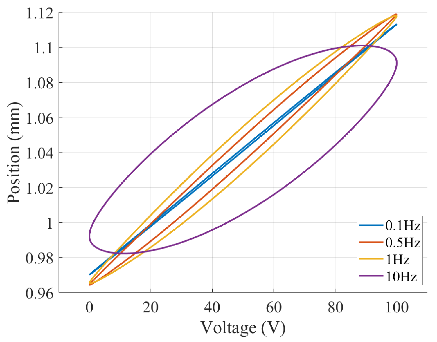
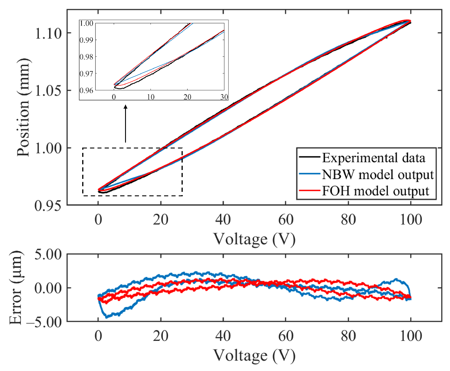
4.2. The FOH Model Parameters Identification

In the traditional hysteresis model, high-order differential equations are often used to describe nonlinear hysteresis [18,50]. It is difficult to identify and highly dependent on the accuracy of nonlinear differential equation mathematical realization. Furthermore, due to the coupling effect of hysteresis and creep nonlinearity in the PEA system, it is difficult to determine the parameters in the hysteresis model.

In this work, the hysteresis of piezoelectric ceramics is modeled as fractional-order dynamics, and the relationship between input and output can be directly used for system identification after fractional-order modeling of hysteresis and decoupling identification of creep effects. There are some existing methods for identifying the hysteresis model, including the minimum mean method, genetic algorithm, and particle swarm optimization (PSO) algorithm [50].

We employ the PSO algorithm to determine the five parameters governing the established hysteresis model, as expressed in Equations (8) and (9). The numerical simulation of fractional-order operators is conducted through the application of a high-precision approximate calculation method for the Caputo definition, along with the utilization of a dedicated implementation tool for fractional-order differentiators. The PSO fitness function is defined as the root-mean-square trajectory tracking error ($e_{RMS}$), serving as a quantitative measure to reflect modeling deviation. Additionally, the relative error index ($e_r$), quantifying the disparity between estimated and experimentally measured displacements, is introduced as an auxiliary reference. The two formulas are expressed as follows:

$$e_{RMS}\left(\Theta \right)=\sqrt{\frac{1}{n}\sum _{i=1}^n{\left(y_i-{\widehat{y}}_i\right)}^2}$$

(12)

$$e_r=\frac{∥y-\widehat{y}∥}{∥y∥}$$

(13)

where the parameter vector $\Theta =[k_l,k_h,\alpha ,k_p,\beta ]$ is the target for determination. The Euclidean norm, denoted by $∥·∥$, is employed to measure the magnitude of the vector. Here, y represents the experimental displacement, $\widehat{y}$ signifies the simulated displacement, and n denotes the total number of data points. The variable i represents the sequential index of the measured data.

The identification procedure employs sinusoidal input signals of 100 V and records the corresponding displacement response at a frequency of 1 Hz for parameter estimation. Throughout this process, both the coefficients and fractional power of the proposed model are concurrently confirmed. The PSO algorithm is iteratively optimized for this purpose, and the parameter identification results for the FOH model are acquired upon convergence of the cost function value. A summary of these results is presented in

Table 1. Parameter identification results of FOH model.

FOH Model
$k_l$	−0.0017418
$k_h$	0.0044141
$k_p$	0.02729
$\alpha$	0.02729
$\beta$	−0.13501
$e_{RMS}$	1.11008‰

.

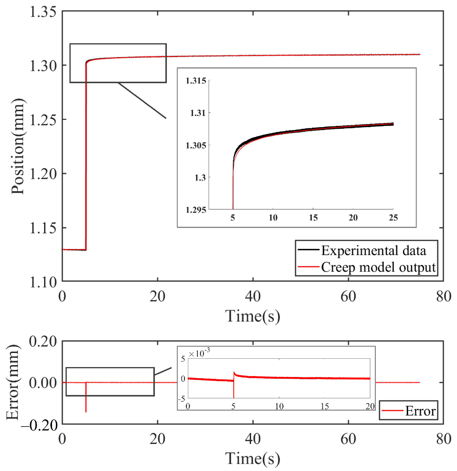
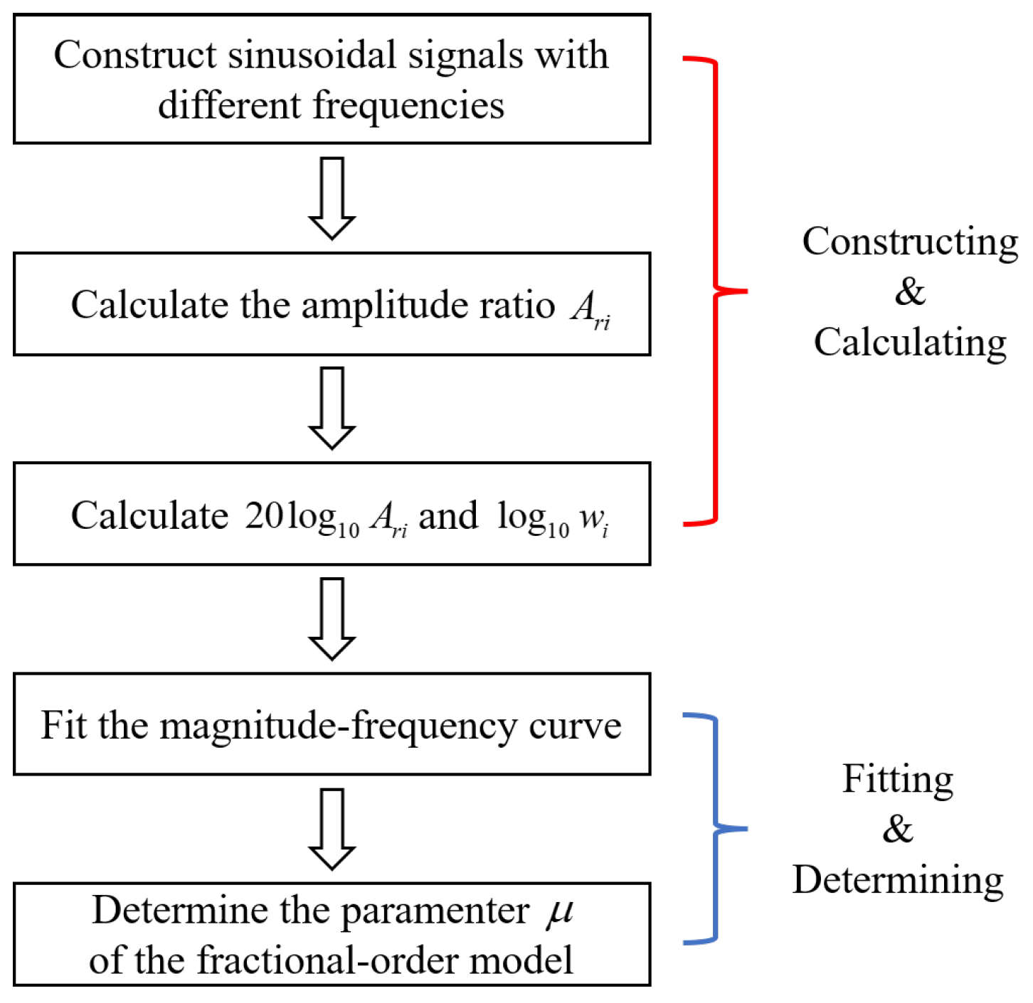
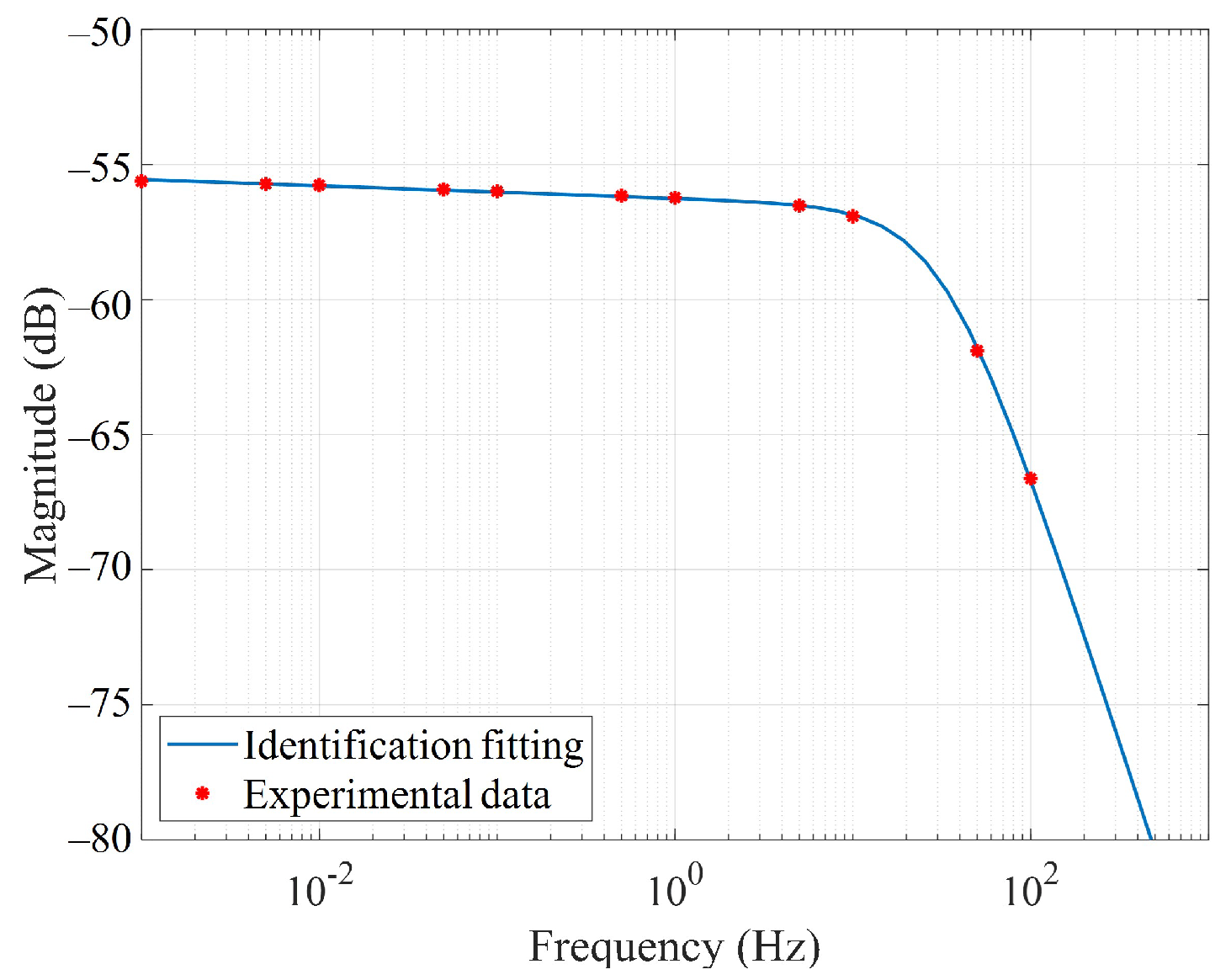
4.3. Fractional-Order Creep Model Parameter Identification

The mentioned creep model is identified by harnessing the dynamic characteristics inherent in fractional power. Figure 15 depicts the flowchart for the identification process of creep system parameters. Initially, sinusoidal signals with various frequencies $w_i\left(i=1,2,\dots ,n\right)$ are generated. Subsequently, the amplitude ratio $A_r$ at each frequency is calculated by

$$A_{ri}=\frac{C_i}{R_i}$$

(14)

$$y_i=20{log}_{10}{A}_{ri}$$

(15)

$$x_i={log}_{10}{w}_i$$

(16)

where $R_i$ and $C_i$ denote the amplitudes of the input and the output at $w_i$, respectively. By defining $y=20{log}_{10}{A}_r$ and $x={log}_{10}w$, the values of $y_i$ and $x_i$ can be computed using Equations (15) and (16).

The identification of the creep link in this section is different from the previous studies. The relationship between y and x is no longer regarded as linear, but the dynamic of the integrated structure of the PEA is taken into account. The fractional-order creep model and the dynamic equation of PEA are combined for parameter identification. This identification method can eliminate the interference of actuator dynamics and improve the identification accuracy of creep link.

The PEA utilized for creep parameter identification in this section is illustrated in Figure 16a. This PEA features an integrated design structure comprising a piezo stack and a flexure hinge. The amalgamated system closely resembles the configuration of a damping mass–spring system, as portrayed in Figure 16b. Deriving from Newton’s second law of motion, the governing differential equation for the PEA is shown as follows:

$$m\ddot{x}\left(t\right)+\left(c_p+c\right)\dot{x}\left(t\right)+\left(k_p+k\right)x\left(t\right)=F_p\left(t\right)$$

(17)

where m represents the equal mass of the PEA, $x\left(t\right)$ denotes the displacement output of the PEA, and c and $c_p$ represent the damping coefficients associated with the flexure hinge and the piezo stack, respectively. Additionally, k and $k_p$ represent the equal stiffness of the hinge and the piezo stack, respectively.

The term $F_p\left(t\right)$ designates the external force applied to the piezo stack and can be formulated as

$$F_p\left(t\right)=n{d}_{33}{k}_p{U}_p\left(t\right)={k_p}^{\prime }{U}_p\left(t\right)$$

(18)

where n signifies the number of the piezo stack layers, and $d_{33}$ represents the piezoelectric constant.

Due to the constancy of these terms, including $k_p$, these three constants are collectively treated as a unified constant denoted as ${k_p}^{\prime }$ during the identification process. The voltage applied to the piezo stack is represented by $U_p\left(t\right)$. Equation (18) relies on a linear assumption, but the inclusion of nonlinear effects is crucial. To address this, a fractional-order system equation describing the creep links of PEAs is formulated by synthesizing the fractional creep links discussed earlier. This equation is given as

$$F_p\left(t\right)={k_p}^{\prime }{U}_p\left(t\right)+a·D_t^{\mu }{U}_p\left(t\right)$$

(19)

where $\mu$ is the differential orders of the applied voltage, and parameter a is a constant gain.

Then, taking the Laplace transform of Equations (17) and (19), the transfer function for the PEA creep system is derived as

$$\begin{array}{cc}\hfill G\left(s\right)& =\frac{X\left(s\right)}{U\left(s\right)}\hfill \\ \hfill & =\left({k_p}^{\prime }+a{s}^{\mu }\right)\left(\frac{1}{m{s}^2+\left(c+c_p\right)s+\left(k+k_p\right)}\right)\hfill \end{array}$$

(20)

where s represents the Laplace operator, and $X\left(s\right)$ and $U\left(s\right)$ correspond to the Laplace transformations of $x\left(t\right)$ and $U_p\left(t\right)$, respectively. The obtained frequency-domain amplitude spectrum of the system is then fitted to the experimental creep amplitude–frequency data, as depicted in Figure 17. Subsequently, the creep parameter is determined, marking the completion of the fractional-order creep model identification process.

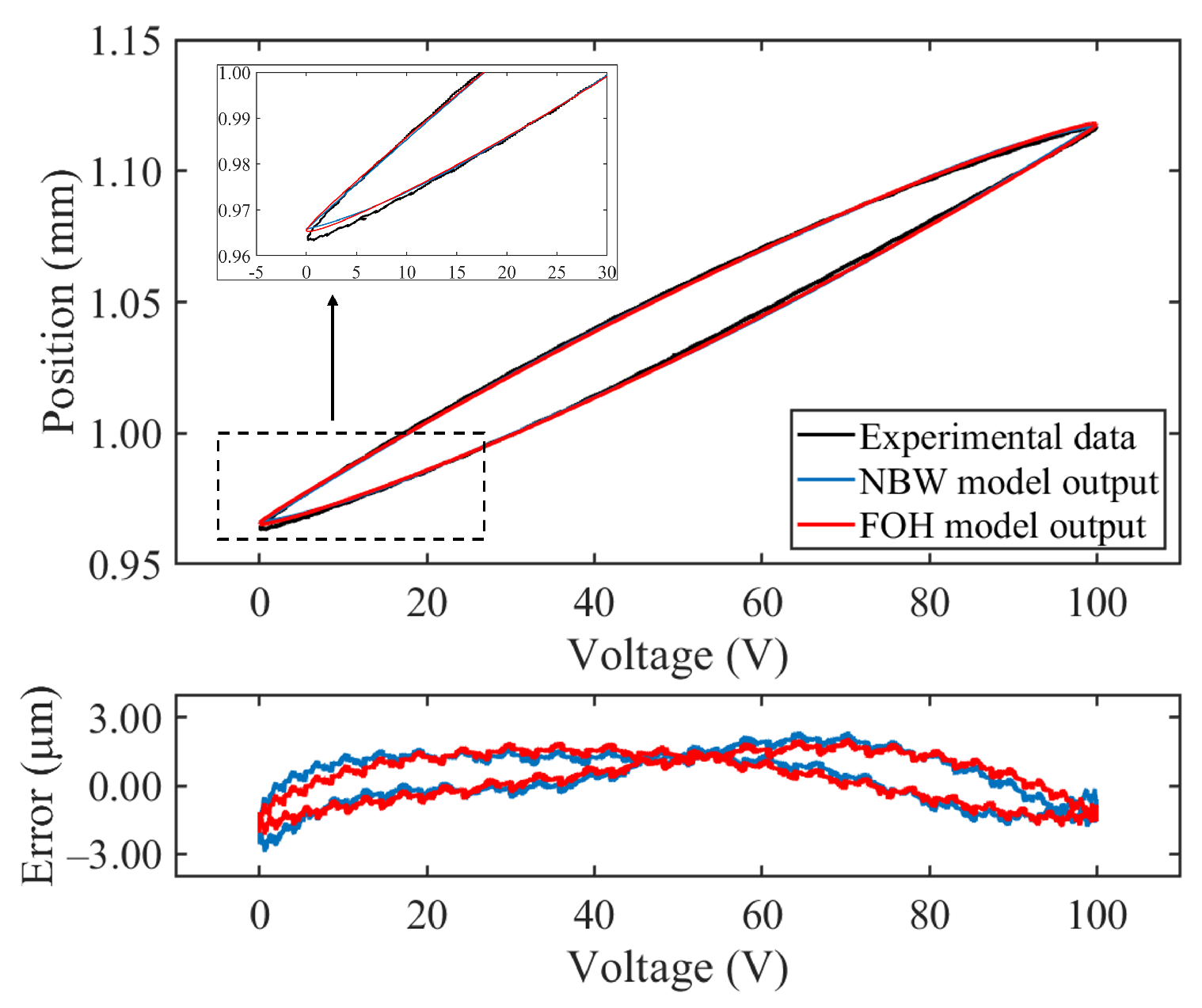
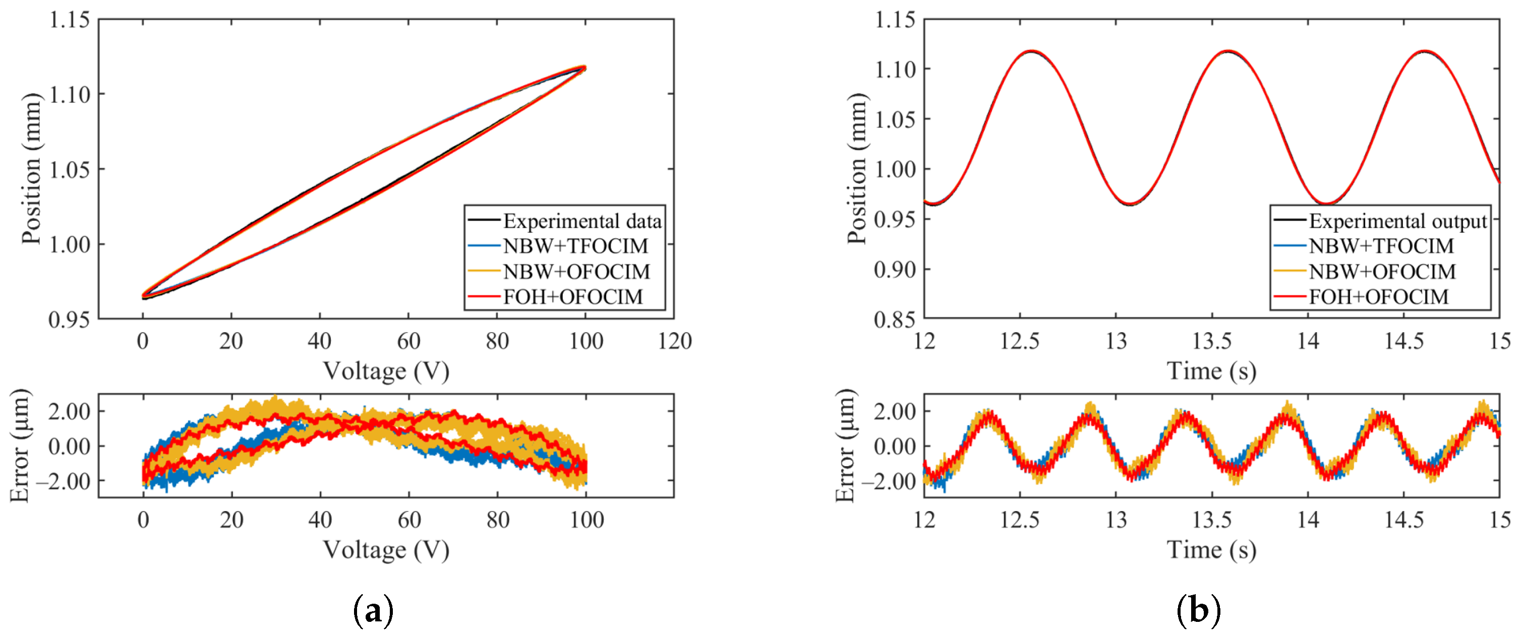
4.4. Experimental Validation of the Models

The results of the hysteresis models are first compared. In Figure 18 and Figure 19, the piezoelectric hysteresis effect of the model is compared with the experimental results under sinusoidal and triangular inputs, respectively. The graphs also show the corresponding prediction errors. As a comparison, the parameters of the normalized Bouc–Wen (NBW) model in [51,52] are determined using the same identification method for the FOH model. The structure of the NBW model is:

$$H\left(u,t\right)=k_{u}u\left(t\right)+k_{h}h\left(t\right)$$

(21)

$$\dot{h}=\rho \left(\dot{u}-\sigma \left|\dot{u}\right|{\left|h\right|}^{n-1}h+\left(\sigma -1\right)·\dot{u}{\left|h\right|}^n\right)$$

(22)

where $u\left(t\right)$ signifies the input voltage to the PEA. The hysteresis displacement output, denoted by $H\left(u,t\right)$, comprises an elastic term $k_{u}u\left(t\right)$ and a pure hysteresis term $k_{h}h\left(t\right)$, characterized by parameters $k_u$ and $k_h$. The auxiliary hysteresis variable, $h\left(t\right)$, is a solution to a nonlinear first-order differential equation (Equation (22)). The shape and magnitude of $h\left(t\right)$ are dictated by parameters $\rho$, $\sigma$, and $n\left(n\ge 1\right)$. The parameter identification results are shown in

Table 2. Parameter identification results of NBW model.

NBW Model
$k_u$	0.0021924
$k_h$	−0.040845
$\rho$	0.19028
$\sigma$	1.288
n	1.6504
$e_{RMS}$	1.1973‰

.

As [52] reported, this NBW model can accurately describe the rate-independent properties of piezoelectric hysteresis. Figure 18 and Figure 19 also show the corresponding fitting results and prediction errors for the comparison. Quantitatively,

Table 3. Quantitative comparison of tracking errors of different models under specific input.

Input Signal	Type	${\mathit{e}}_{\mathbf{RMS}}$	${\mathit{e}}_{\mathit{r}}$
Sinusoidal input	NBW model	1.19773e‰	0.764227‰
	FOH model	1.11008‰	0.708572‰
	Improvement	7.31801%	7.28252%
Triangular input	NBW model	1.35698‰	1.208703‰
	FOH model	0.90145‰	0.802953‰
	Improvement	33.56903 %	33.56904%

lists the $e_{RMS}$ of the FOH model and the NBW model of the experimental PEA system. It can be seen that, when compared with the NBW model, the FOH model outperforms it in the static piezoelectric hysteresis loop under different input conditions. In the sinusoidal case, the model’s accuracy improves by 7.3%; with the triangular wave input, the tracking accuracy improves by 33.569%.

Following the validation of the hysteresis model, an experiment was conducted to compare the output displacement of the actual PEA with the identified fractional-order model. This aimed to further confirm and substantiate the established creep–hysteresis coupled fractional-order model. To gauge the advancements in tracking progress facilitated by the optimized fractional-order creep link identification method (OFOCIM), a set of experiments with the traditional fractional-order creep link identification method (TFOCIM) was included for comparative analysis. Three experiments were performed using a consistent 1 Hz frequency and a 100 V sinusoidal input signal. Coupled Model-1 was formed by integrating the NBW model with the fractional-order creep model using TFOCIM. Coupled Model-2 resulted from coupling the NBW model and the fractional-order creep model through OFOCIM. Coupled Model-3 emerged from the coupling of the FOH model with OFOCIM. Figure 20 illustrates the fitting curves and prediction errors, while

Table 4. Quantitative comparison of tracking errors of different coupled models.

Coupling Type	${\mathit{e}}_{\mathbf{RMS}}$	${\mathit{e}}_{\mathit{r}}$
NBW + TFOCIM	1.152877‰	0.735807‰
NBW + OFOCIM	1.152490‰	0.735588‰
Improvement	0.0335682%	0.029763%
FOH + OFOCIM	1.10993‰	0.708479‰
Improvement	3.7252%	3.71402%

provides the $e_{RMS}$ and relative error $e_r$.

From a quantitative standpoint, as depicted in Figure 20 and detailed in Table 4, it is evident that the accuracy of the coupled NBW + OFOCIM model surpasses that of the original NBW + TFOCIM model by 0.0336%. This result substantiates the enhanced accuracy achieved through the altered identification method within the coupled model. Specifically, the proposed coupled model exhibits a notable advancement of 3.7252% in nonlinear tracking accuracy compared to its predecessor, emphasizing its efficacy in capturing intricate hysteresis and creep phenomena in PEAs.

Consequently, the findings underscore the capability of the introduced coupled hysteresis and creep model to achieve superior modeling accuracy when juxtaposed with conventional models. However, it is worth noting that fractional-order computations typically entail increased hardware resource requirements compared to traditional computations. This consideration emphasizes the importance of balancing modeling benefits with resource demands, ensuring the judicious selection of models based on the specific constraints and goals of practical applications.

5. Conclusions

In this paper, to provide an accurate dynamic description of PEAs, a unique fractional-order model that can adequately capture hysteresis- and creep-coupled effects is proposed. The proposed fractional-order coupled model can track hysteresis and creep nonlinear characteristics such as piezoelectric lag, non-local memory, peak transition, and creep amplitude–frequency features with high accuracy using only six parameters. Based on these characteristics, an identification method is proposed using the PSO algorithm for identification. With the proposed fractional-order model and identification for PEAs, the $e_{RMS}$ of the nonlinear displacement output of the model can be reduced by 3.7253% and the relative error can be reduced by 3.714% in comparison to the NBW coupled model. The superiority of the proposed coupled model in hysteresis and creep nonlinear characteristics tracking accuracy is verified by simulation and experimental demonstration, which is beneficial for using this model to compensate and improve the positioning and motion performance of PEAs.

References

1. Jang, D.D.; Jung, H.J.; Shin, Y.H.; Moon, S.J.; Moon, Y.J.; Oh, J. Feasibility study on a hybrid mount system with air springs and piezo-stack actuators for micro-vibration control. J. Intell. Mater. Syst. Struct. 2012, 23, 515–526. [Google Scholar] [CrossRef]
2. Wang, C.; Lu, Q.; Zhang, K.; Shao, L. Design of micro-vibration suppression platform based on piezo-stack array intelligent structure. Proc. Inst. Mech. Eng. Part C J. Mech. Eng. Sci. 2023, 237, 799–810. [Google Scholar] [CrossRef]
3. Zhiyuan, G.; Muyao, S.; Yiru, W.; Xiaojin, Z. Hybrid De-Jaya Optimized Variable Step-Size and Tap-Length Adaptive Filtering Control Algorithm Active Micro-vibration Control with Piezoelectric Stack Actuator. J. Vib. Eng. Technol. 2022, 10, 887–896. [Google Scholar] [CrossRef]
4. Huang, D.; Min, D.; Jian, Y.; Li, Y. Current-cycle iterative learning control for high-precision position tracking of piezoelectric actuator system via active disturbance rejection control for hysteresis compensation. IEEE Trans. Ind. Electron. 2019, 67, 8680–8690. [Google Scholar] [CrossRef]
5. Fang, J.; Zhang, L.; Long, Z.; Wang, M.Y. Fuzzy adaptive sliding mode control for the precision position of piezo-actuated nano positioning stage. Int. J. Precis. Eng. Manuf. 2018, 19, 1447–1456. [Google Scholar] [CrossRef]
6. Wang, Z.L.; Wu, W.; Falconi, C. Piezotronics and piezo-phototronics with third-generation semiconductors. MRS Bull. 2018, 43, 922–927. [Google Scholar] [CrossRef]
7. Sun, C.; Wu, F.; Wallis, D.J.; Shen, M.H.; Yuan, F.; Yang, J.; Wu, J.; Xie, Z.; Liang, D.; Wang, H.; et al. Gallium nitride: A versatile compound semiconductor as novel piezoelectric film for acoustic tweezer in manipulation of cancer cells. IEEE Trans. Electron Devices 2020, 67, 3355–3361. [Google Scholar] [CrossRef]
8. Shan, G.; Zhu, M. A piezo stack energy harvester with frequency up-conversion for rail track vibration. Mech. Syst. Signal Process. 2022, 178, 109268. [Google Scholar] [CrossRef]
9. Wen, Z.; Ding, Y.; Liu, P.; Ding, H. An efficient identification method for dynamic systems with coupled hysteresis and linear dynamics: Application to piezoelectric-actuated nanopositioning stages. IEEE/ASME Trans. Mechatron. 2019, 24, 326–337. [Google Scholar] [CrossRef]
10. Ando, T. High-speed atomic force microscopy. Curr. Opin. Chem. Biol. 2019, 51, 105–112. [Google Scholar] [CrossRef]
11. Habibullah; Pota, H.R.; Petersen, I.R.; Rana, M.S. Creep, Hysteresis, and Cross-Coupling Reduction in the High-Precision Positioning of the Piezoelectric Scanner Stage of an Atomic Force Microscope. IEEE Trans. Nanotechnol. 2013, 12, 1125–1134. [Google Scholar] [CrossRef]
12. Li, Y.; Xu, Q. Adaptive Sliding Mode Control With Perturbation Estimation and PID Sliding Surface for Motion Tracking of a Piezo-Driven Micromanipulator. IEEE Trans. Control Syst. Technol. 2010, 18, 798–810. [Google Scholar] [CrossRef]
13. Grzybek, D.; Sioma, A. Creep Phenomenon in a Multiple-Input Single-Output Control System of a Piezoelectric Bimorph Actuator. Energies 2022, 15, 8267. [Google Scholar] [CrossRef]
14. Richter, H.; Misawa, E.; Lucca, D.; Lu, H. Modeling nonlinear behavior in a piezoelectric actuator. Precis. Eng. 2001, 25, 128–137. [Google Scholar] [CrossRef]
15. Grech, C.; Buzio, M.; Pentella, M.; Sammut, N. Dynamic ferromagnetic hysteresis modelling using a Preisach-recurrent neural network model. Materials 2020, 13, 2561. [Google Scholar] [CrossRef] [PubMed]
16. Rosenbaum, S.; Ruderman, M.; Strohla, T.; Bertram, T. Use of Jiles–Atherton and Preisach Hysteresis Models for Inverse Feed-Forward Control. IEEE Trans. Magn. 2010, 46, 3984–3989. [Google Scholar] [CrossRef]
17. Li, Z.; Xiong, L.; Tang, L.; Yang, W.; Liu, K.; Mace, B. Modeling and harmonic analysis of energy extracting performance of a piezoelectric nonlinear energy sink system with AC and DC interface circuits. Mech. Syst. Signal Process. 2021, 155, 107609. [Google Scholar] [CrossRef]
18. Fujii, F.; Tatebatake, K.; Morita, K.; Shiinoki, T. A Bouc-Wen model-based compensation of the frequency-dependent hysteresis of a piezoelectric actuator exhibiting odd harmonic oscillation. Actuators 2018, 7, 37. [Google Scholar] [CrossRef]
19. Habineza, D.; Rakotondrabe, M.; Le Gorrec, Y. Bouc–Wen Modeling and Feedforward Control of Multivariable Hysteresis in Piezoelectric Systems: Application to a 3-DOF Piezotube Scanner. IEEE Trans. Control Syst. Technol. 2015, 23, 1797–1806. [Google Scholar] [CrossRef]
20. Xie, S.L.; Liu, H.T.; Mei, J.P.; Gu, G.Y. Modeling and compensation of asymmetric hysteresis for pneumatic artificial muscles with a modified generalized Prandtl–Ishlinskii model. Mechatronics 2018, 52, 49–57. [Google Scholar] [CrossRef]
21. Wang, W.; Wang, R.; Chen, Z.; Sang, Z.; Lu, K.; Han, F.; Wang, J.; Ju, B. A new hysteresis modeling and optimization for piezoelectric actuators based on asymmetric Prandtl-Ishlinskii model. Sens. Actuators A Phys. 2020, 316, 112431. [Google Scholar] [CrossRef]
22. Xiao, S.; Li, Y. Modeling and High Dynamic Compensating the Rate-Dependent Hysteresis of Piezoelectric Actuators via a Novel Modified Inverse Preisach Model. IEEE Trans. Control Syst. Technol. 2013, 21, 1549–1557. [Google Scholar] [CrossRef]
23. Zhang, X.; Tan, Y.; Su, M. Modeling of hysteresis in piezoelectric actuators using neural networks. Mech. Syst. Signal Process. 2009, 23, 2699–2711. [Google Scholar] [CrossRef]
24. Dang, X.; Tan, Y. RBF neural networks hysteresis modelling for piezoceramic actuator using hybrid model. Mech. Syst. Signal Process. 2007, 21, 430–440. [Google Scholar] [CrossRef]
25. Jung, H.; Gweon, D.G. Creep characteristics of piezoelectric actuators. Rev. Sci. Instruments 2000, 71, 1896–1900. [Google Scholar] [CrossRef]
26. Changhai, R.; Lining, S. Hysteresis and creep compensation for piezoelectric actuator in open-loop operation. Sens. Actuators A Phys. 2005, 122, 124–130. [Google Scholar] [CrossRef]
27. Georgiou, H.; Mrad, R.B. Dynamic electromechanical drift model for PZT. Mechatronics 2008, 18, 81–89. [Google Scholar] [CrossRef]
28. Gu, G.Y.; Zhu, L.M. Motion control of piezoceramic actuators with creep, hysteresis and vibration compensation. Sens. Actuators A Phys. 2013, 197, 76–87. [Google Scholar] [CrossRef]
29. Lapchuk, A.; Yun, S.K.; An, S.; Song, J.; Yurlov, V.; Bourim, E.; Yang, H.; Park, H. Creep compensation method in a thin film PZT structure for a spatial optical modulator. Sens. Actuators A Phys. 2011, 167, 406–415. [Google Scholar] [CrossRef]
30. Cao, Y.; Chen, X.B. A Survey of Modeling and Control Issues for Piezo-electric Actuators. J. Dyn. Syst. Meas. Control 2014, 137, 014001. [Google Scholar] [CrossRef]
31. Liu, L.; Tan, K.K.; Teo, C.S.; Chen, S.L.; Lee, T.H. Development of an Approach Toward Comprehensive Identification of Hysteretic Dynamics in Piezoelectric Actuators. IEEE Trans. Control Syst. Technol. 2013, 21, 1834–1845. [Google Scholar] [CrossRef]
32. Liu, Y.; Shan, J.; Qi, N. Creep modeling and identification for piezoelectric actuators based on fractional-order system. Mechatronics 2013, 23, 840–847. [Google Scholar] [CrossRef]
33. Wen, Z.; Ding, Y.; Liu, P.; Ding, H. Direct integration method for time-delayed control of second-order dynamic systems. J. Dyn. Syst. Meas. Control 2017, 139, 061001. [Google Scholar] [CrossRef]
34. Liu, L.; Yun, H.; Li, Q.; Ma, X.; Chen, S.L.; Shen, J. Fractional Order Based Modeling and Identification of Coupled Creep and Hysteresis Effects in Piezoelectric Actuators. IEEE/ASME Trans. Mechatron. 2020, 25, 1036–1044. [Google Scholar] [CrossRef]
35. Hilfer, R. Fractional diffusion based on Riemann-Liouville fractional derivatives. J. Phys. Chem. B 2000, 104, 3914–3917. [Google Scholar] [CrossRef]
36. Scherer, R.; Kalla, S.L.; Tang, Y.; Huang, J. The Grünwald–Letnikov method for fractional differential equations. Comput. Math. Appl. 2011, 62, 902–917. [Google Scholar] [CrossRef]
37. Xue, D. Fractional Calculus and Fractional-Order Control; Science Press: Beijing, China, 2018. [Google Scholar]
38. Nonnenmacher, T.F.; Metzler, R. On the Riemann-Liouville fractional calculus and some recent applications. Fractals 1995, 3, 557–566. [Google Scholar] [CrossRef]
39. Garg, V.; Singh, K. An improved Grunwald-Letnikov fractional differential mask for image texture enhancement. Int. J. Adv. Comput. Sci. Appl. 2012, 3. [Google Scholar] [CrossRef]
40. Chakraborty, M.; Maiti, D.; Konar, A.; Janarthanan, R. A study of the Grunwald-Letnikov definition for minimizing the effects of random noise on fractional order differential equations. In Proceedings of the 2008 4th International Conference on Information and Automation for Sustainability, Colombo, Sri Lanka, 12–14 December 2008; pp. 449–456. [Google Scholar]
41. Oustaloup, A.; Moreau, X.; Nouillant, M. The CRONE suspension. Control Eng. Pract. 1996, 4, 1101–1108. [Google Scholar] [CrossRef]
42. Sar, E.Y.; Giresunlu, I.B. Fractional differential equations. Pramana J. Phys 2016, 87, 17. [Google Scholar]
43. Caputo, M. Linear models of dissipation whose Q is almost frequency independent-II. Geophys. J. Int. 1967, 13, 529–539. [Google Scholar] [CrossRef]
44. Merrikh-Bayat, F. Rules for selecting the parameters of Oustaloup recursive approximation for the simulation of linear feedback systems containing PIλDμ controller. Commun. Nonlinear Sci. Numer. Simul. 2012, 17, 1852–1861. [Google Scholar] [CrossRef]
45. Fang, J.; Yin, Z. Dielectric Physics; Science Press: Beijing, China, 1989; pp. 261–303. [Google Scholar]
46. Auciello, O.; Scott, J.F.; Ramesh, R. The physics of ferroelectric memories. Phys. Today 1998, 51, 22–27. [Google Scholar] [CrossRef]
47. Wang Chunlei, L.J.; Minglei, Z. Piezoelectric Ferroelectric Physics; Science Press of China: Beijing, China, 2009. [Google Scholar]
48. Huang, C.; Cai, K.; Wang, Y.; Bai, Y.; Guo, D. Revealing the real high temperature performance and depolarization characteristics of piezoelectric ceramics by combined in situ techniques. J. Mater. Chem. C 2018, 6, 1433–1444. [Google Scholar] [CrossRef]
49. Brokate, M.; Sprekels, J. Hysteresis and Phase Transitions; Springer Science & Business Media: Berlin/Heidelberg, Germany, 1996; Volume 121. [Google Scholar]
50. Hassani, V.; Tjahjowidodo, T.; Do, T.N. A survey on hysteresis modeling, identification and control. Mech. Syst. Signal Process. 2014, 49, 209–233. [Google Scholar] [CrossRef]
51. Ikhouane, F.; Hurtado, J.E.; Rodellar, J. Variation of the hysteresis loop with the Bouc-Wen model parameters. Nonlinear Dyn. 2007, 48, 361–380. [Google Scholar] [CrossRef]
52. Kang, S.; Wu, H.; Li, Y.; Yang, X.; Yao, J. A Fractional-Order Normalized Bouc-Wen Model for Piezoelectric Hysteresis Nonlinearity. IEEE/ASME Trans. Mechatron. 2021, 27, 126–136. [Google Scholar] [CrossRef]
Figure 1. Simulation of fractional-order operators under bidirectional displacement signal input signal. (a) Fractional-order operator simulation of input x t and output y t . (b) Fractional-order operator hysteresis loop of output y t –input x t .
Fractalfract 08 00003 g001
Figure 2. Measured hysteresis curve of a PEA driven by the 1 Hz sinusoidal voltage.
Fractalfract 08 00003 g002
Figure 3. The time-domain signal of a 1 Hz sinusoidal voltage applied to the PEA.
Fractalfract 08 00003 g003
Figure 4. The hysteresis curve is conceptualized as an illustrative diagram depicting the linear and nonlinear modules.
Fractalfract 08 00003 g004
Figure 5. The structure diagram of the fractional-order hysteresis model.
Fractalfract 08 00003 g005
Figure 6. Frequency domain similarity between ideal fractional-order system and high-order Oustaloup method.
Fractalfract 08 00003 g006
Figure 7. Structure of the proposed coupled model.
Fractalfract 08 00003 g007
Figure 8. Measurement results of high-temperature ferroelectric hysteresis loops.
Fractalfract 08 00003 g008
Figure 9. Representation of peak transition behavior by FOH model.
Fractalfract 08 00003 g009
Figure 10. Hysteresis characteristics of the FOH model. (a) Gauss pulse signal voltage input. (b) Experimental phenomena and model simulation output of non-local memory effect.
Fractalfract 08 00003 g010
Figure 11. Performance of experimental creep behavior and fractional-order creep model output.
Fractalfract 08 00003 g011
Figure 12. The Bode diagram of the fractional-order creep model system.
Fractalfract 08 00003 g012
Figure 13. Features of the fractional-order coupled model under different low-frequency sine signal inputs.
Fractalfract 08 00003 g013
Figure 14. Experimental instruments and settings.
Fractalfract 08 00003 g014
Figure 15. Parameter identification approach of the fractional-order creep model.
Fractalfract 08 00003 g015
Figure 16. The dynamic equivalence model of the PEA. (a) Composition structure schematic representation of PEA. (b) Equivalent mechanical dynamics model.
Fractalfract 08 00003 g016
Figure 17. Identification diagram of creep amplitude–frequency spectrum.
Fractalfract 08 00003 g017
Figure 18. Hysteretic tracking effect and error of the FOH model under sinusoidal input.
Fractalfract 08 00003 g018
Figure 19. Hysteretic tracking effect and error of the FOH model under triangular input.
Fractalfract 08 00003 g019
Figure 20. Hysteresis loops and time-domain tracking effects of three coupled models. (a) Hysteresis loops tracking effect. (b) Time-domain tracking effect.
Fractalfract 08 00003 g020