

On Extended Class of Totally Ordered Interval-Valued Convex Stochastic Processes and Applications
 , , ,
, , ,  and
and
Abstract
:1. Introduction and Preliminaries
Stochastic Analysis
- P-upper bounded on if
- P-lower bounded on if
- P-bounded if it is P-upper and lower bounded on .
- Continuous on I, if ,where P-limit denotes the limit in probability space.
- Mean square continuous in I, ifand represents the expectation of random variable .
- Mean square differentiable at if there exists a random variable , such that
- Process is a mean square integrable with . The random variable is a mean square integral of if for each partition of such that and for all , we have
2. Results and Discussions
2.1. Analysis of Extended Class of Convex Stochastic Process
- Selecting in Definition 6, we obtain a convex stochastic process:
- Selecting in Definition 6, we obtain a convex stochastic process:
- Selecting in Definition 6, we obtain a Godunova–Levin convex stochastic process:
- Selecting in Definition 6, we obtain a Godunova–Levin convex stochastic process:
- Selecting in Definition 6, we obtain a tgs convex stochastic process:
- Selecting in Definition 6, we obtain a Q-convex stochastic process:
- Selecting and in Definition 6, we obtain a convex stochastic process:
- Selecting and in Definition 6, we obtain a convex stochastic process:
- Selecting and in Definition 6, we obtain a convex stochastic process:
- Selecting and in Definition 6, we obtain a Godunova-Levin convex stochastic process:
- Selecting and in Definition 6, we obtain a tgs convex stochastic process:
- Selecting in Definition 6, we obtain a harmonic convex stochastic process:
- Selecting and in Definition 6, we obtain a harmonic convex stochastic process:
- Selecting and in Definition 6, we obtain a convex stochastic process:
- Selecting and in Definition 6, we obtain a harmonic convex stochastic process:
- Selecting and in Definition 6, we obtain a Godunova-Levin harmonic convex stochastic process:
- Selecting and in Definition 6, we obtain a harmonic convex stochastic process:
- Selecting , in Definition 6, we obtain a convex stochastic process:
- Selecting and in Definition 6, we obtain a convex stochastic process:
- Selecting and in Definition 6, we obtain a Godunova–Levin convex stochastic process:
- Selecting and in Definition 6, we obtain a convex stochastic process:
- Selecting and in Definition 6, we obtain a convex stochastic process:
- Selecting and in Definition 6, we obtain a Godunova–Levin convex stochastic process:
- (a)
- .
- (b)
- for .
- Selecting in Theorem 4, then we acquire Jensen’s inequality for a -convex stochastic process,
- Selecting in Theorem 4, then we acquire the Jensen’s inequality for a harmonically -convex stochastic process,
- Selecting , in Theorem 4, then we acquire Jensen’s inequality for a convex stochastic process,
- Choosing in Theorem 4, we acquire the Jensen’s inequality for a convex stochastic process,
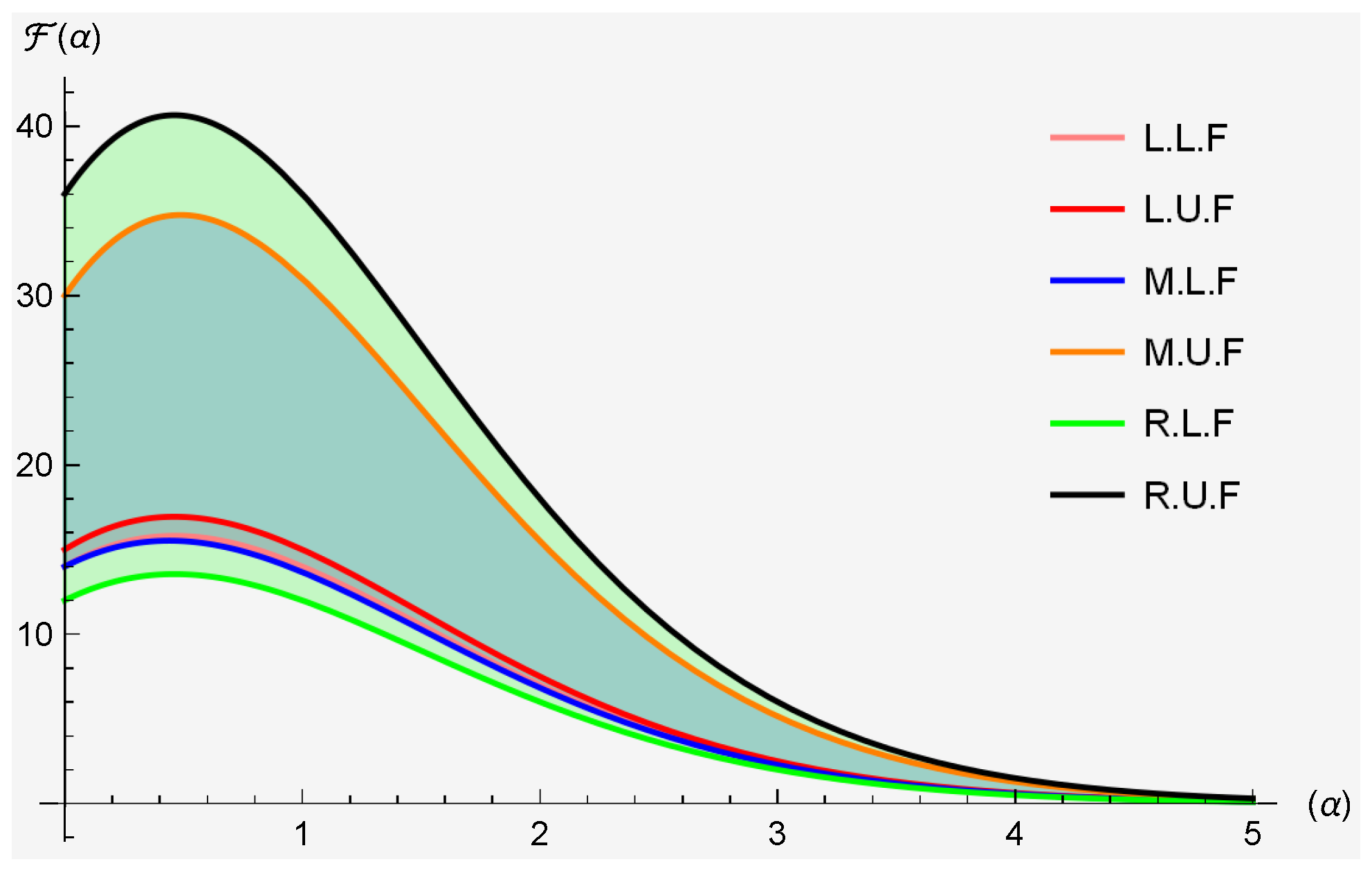
- Selecting in Theorem 5, we achieve
- Selecting in Theorem 5, we obtainwhere is a well-known beta function.
- Choosing , in Theorem 5, we acquire
- Choosing , and in Theorem 5, we acquirewhere .
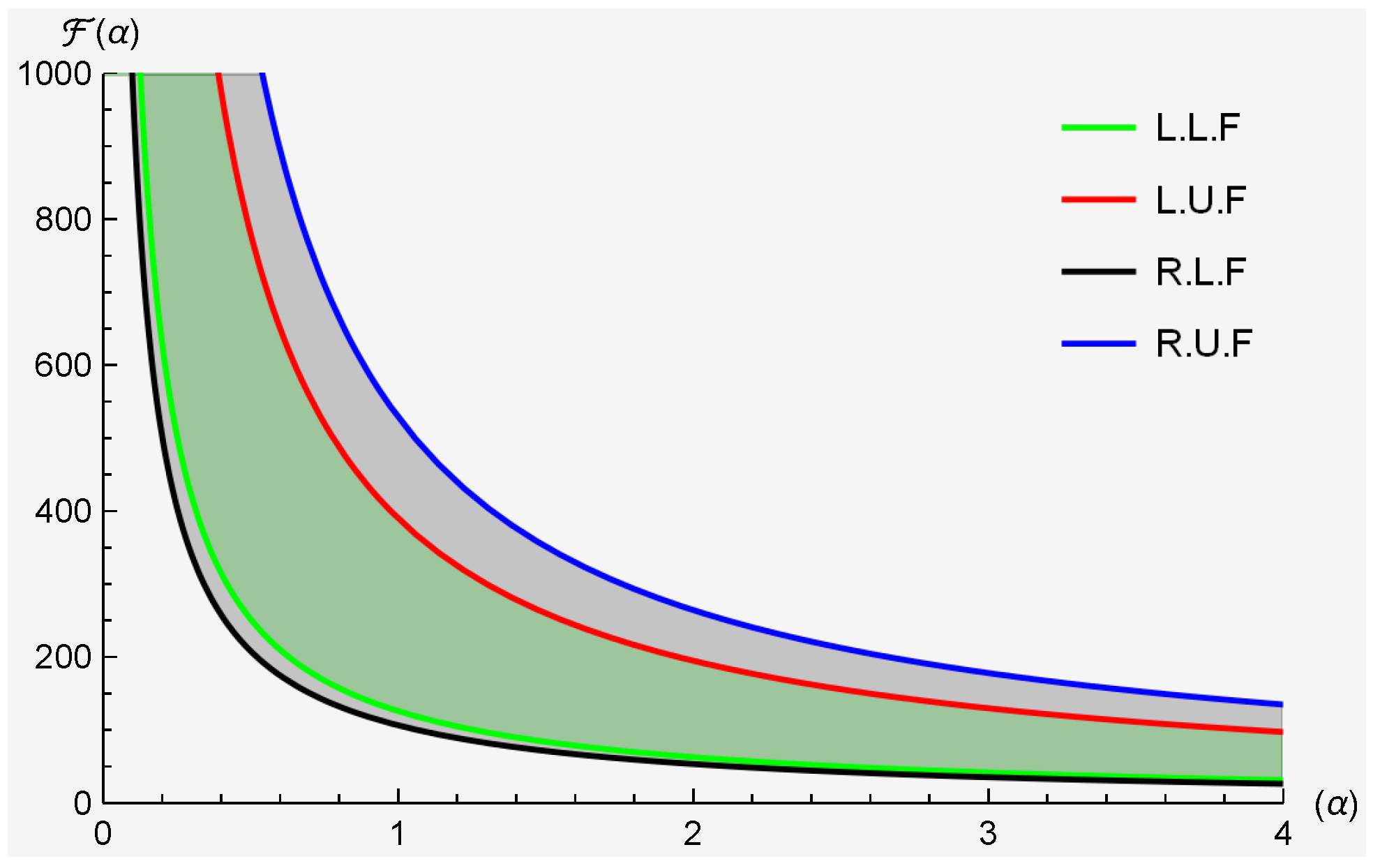
- Choosing in Theorem 6, we haveand .
- Choosing and in Theorem 6, thenand .
- Choosing in Theorem 6, thenand .
- If we choose and in Theorem 6, thenand .
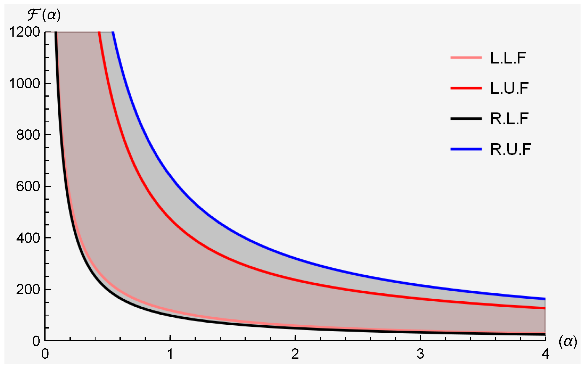
- Choosing in Theorem 7, then
- Choosing and in Theorem 7, then
- Choosing and in Theorem 7, then
- Choosing in Theorem 8, thenwhere and are given by (13) and (14), respectively.
- Choosing and in Theorem 8, thenwhere and are given by (13) and (14), respectively.
- Choosing and in Theorem 8, thenwhere and are given by (13) and (14), respectively.
2.2. Applicable Analysis
- The arithmetic mean:
- The generalized log-mean:
3. Conclusions
Author Contributions
Funding
Data Availability Statement
Acknowledgments
Conflicts of Interest
References
- Dragomir, S.S.; Pearce, C.E.M. Selected Topics on Hermite–Hadamard Inequalities and Applications; Research Group in Mathematical Inequalities and Applications (RGMIA), Victoria University: Melbourne, Australia, 2000. [Google Scholar]
- Peajcariaac, J.E.; Tong, Y.L. Convex Functions, Partial Orderings, and Statistical Applications; Academic Press: New York, NY, USA, 1992. [Google Scholar]
- El Farissi, A. Simple proof and refinement of Hermite-Hadamard inequality. J. Math. Inequalities 2010, 4, 365–369. [Google Scholar] [CrossRef]
- Gao, X. A note on the Hermite-Hadamard inequality. J. Math. Inequalities 2010, 4, 587–591. [Google Scholar] [CrossRef]
- Wu, S.; Awan, M.U.; Noor, M.A.; Noor, K.I.; Iftikhar, S. On a new class of convex functions and integral inequalities. J. Inequalities Appl. 2019, 2019, 131. [Google Scholar] [CrossRef]
- Moore, R.E. Interval Analysis; Prentice-Hall: Englewood Cliffs, NJ, USA, 1966; Volume 4, pp. 8–13. [Google Scholar]
- Breckner, W.W. Continuity of generalized convex and generalized concave set-valued functions. Rev. Analyse Numer. Theor. Approx. 1993, 22, 39–51. [Google Scholar]
- Bhunia, A.K.; Samanta, S.S. A study of interval metric and its application in multi-objective optimization with interval objectives. Comput. Ind. Eng. 2014, 74, 169–178. [Google Scholar] [CrossRef]
- Shi, F.; Ye, G.; Liu, W.; Zhao, D. cr-h-convexity and some inequalities for cr-h-convex function. ResearchGate 2022. [Google Scholar]
- Zhao, D.; An, T.; Ye, G.; Liu, W. New Jensen and Hermite-Hadamard type inequalities for h-convex interval-valued functions. J. Inequalities Appl. 2018, 2018, 302. [Google Scholar] [CrossRef]
- Zhao, D.; An, T.; Ye, G.; Liu, W. Chebyshev type inequalities for interval-valued functions. Fuzzy Sets Syst. 2020, 396, 82–101. [Google Scholar] [CrossRef]
- Budak, H.; Tunc, T.; Sarikaya, M. Fractional Hermite-Hadamard-type inequalities for interval-valued functions. Proc. Am. Math. Soc. 2020, 148, 705–718. [Google Scholar] [CrossRef]
- Bin-Mohsin, B.; Rafique, S.; Cesarano, C.; Javed, M.Z.; Awan, M.U.; Kashuri, A.; Noor, M.A. Some general fractional integral inequalities involving LR-Bi-convex fuzzy interval-valued functions. Fractal Fract. 2022, 6, 565. [Google Scholar] [CrossRef]
- Bin-Mohsin, B.; Javed, M.Z.; Awan, M.U.; Kashuri, A. On some new AB-fractional inclusion relations. Fractal Fract. 2023, 7, 725. [Google Scholar] [CrossRef]
- Rahman, M.S.; Shaikh, A.A.; Bhunia, A.K. Necessary and sufficient optimality conditions for non-linear unconstrained and constrained optimization problem with interval valued objective function. Comput. Ind. Eng. 2020, 147, 106634. [Google Scholar] [CrossRef]
- Liu, W.; Shi, F.; Ye, G.; Zhao, D. The Properties of Harmonically cr-h-Convex function and Its Applications. Mathematics 2022, 10, 2089. [Google Scholar] [CrossRef]
- Sahoo, S.K.; Latif, M.A.; Alsalami, O.M.; Treanta, S.; Sudsutad, W.; Kongson, J. Hermite-Hadamard, Fejér and Pachpatte-Type integral inequalities for center-radius order interval-valued preinvex functions. Fractal Fract. 2022, 6, 506. [Google Scholar] [CrossRef]
- Vivas-Cortez, M.; Ramzan, S.; Awan, M.U.; Javed, M.Z.; Khan, A.G.; Noor, M.A. IV-CR-γ-Convex functions and Their Application in Fractional Hermite-Hadamard Inequalities. Symmetry 2023, 15, 1405. [Google Scholar] [CrossRef]
- Du, T.; Zhou, T. On the fractional double integral inclusion relations having exponential kernels via interval-valued co-ordinated convex functions. Chaos Solitons Fractals 2022, 156, 111846. [Google Scholar] [CrossRef]
- Chalco-Cano, Y.; Flores-Franulic, A.; Roman-Flores, H. Ostrowski type inequalities for interval-valued functions using generalized Hukuhara derivative. Comput. Appl. Math. 2012, 31, 457–472. [Google Scholar]
- Chalco-Cano, Y.; Lodwick, W.A.; Condori-Equice, W. Ostrowski type inequalities and applications in numerical integration for interval-valued functions. Soft Comput. 2015, 19, 3293–3300. [Google Scholar] [CrossRef]
- Costa, T.M.; Román-Flores, H. Some integral inequalities for fuzzy-interval-valued functions. Inf. Sci. 2017, 420, 110–125. [Google Scholar] [CrossRef]
- Roman-Flores, H.; Chalco-Cano, Y.; Lodwick, W. Some integral inequalities for interval-valued functions. Comput. Appl. Math. 2018, 37, 1306–1318. [Google Scholar] [CrossRef]
- Bin-Mohsin, B.; Awan, M.U.; Javed, M.Z.; Budak, H.; Khan, A.G.; Noor, M.A. Inclusions Involving interval-valued harmonically co-Ordinated convex functions and Raina’s Fractional Double Integrals. J. Math. 2022, 2022, 5815993. [Google Scholar] [CrossRef]
- Bin-Mohsin, B.; Awan, M.U.; Javed, M.Z.; Khan, A.G.; Budak, H.; Mihai, M.V.; Noor, M.A. Generalized AB-fractional operator inclusions of Hermite-Hadamard’s type via fractional integration. Symmetry 2023, 15, 1012. [Google Scholar] [CrossRef]
- Fahad, A.; Wang, Y.; Ali, Z.; Hussain, R.; Furuichi, S. Exploring properties and inequalities for geometrically arithmetically-Cr-convex functions with Cr-order relative entropy. Inf. Sci. 2024, 662, 120219. [Google Scholar] [CrossRef]
- Tong, X.; Jiang, H.; Chen, X.; Li, J.; Cao, Z. Deterministic and stochastic evolution of rumor propagation model with media coverage and class-age-dependent education. Math. Methods Appl. Sci. 2023, 46, 7125–7139. [Google Scholar] [CrossRef]
- Zhang, X.; Liu, E.; Qiu, J.; Zhang, A.; Liu, Z. Output feedback finite-time stabilization of a class of large-scale high-order nonlinear stochastic feedforward systems. Discret. Contin. Dyn. Syst. 2023, 16, 1892–1908. [Google Scholar] [CrossRef]
- Zhang, N.; Qi, W.; Pang, G.; Cheng, J.; Shi, K. Observer-based sliding mode control for fuzzy stochastic switching systems with deception attacks. Appl. Math. Comput. 2022, 427, 127153. [Google Scholar] [CrossRef]
- Yang, C.; Li, F.; Kong, Q.; Chen, X.; Wang, J. Asynchronous fault-tolerant control for stochastic jumping singularly perturbed systems: An H∞ sliding mode control scheme. Appl. Math. Comput. 2021, 389, 125562. [Google Scholar] [CrossRef]
- Jiao, T.; Zong, G.; Pang, G.; Zhang, H.; Jiang, J. Admissibility analysis of stochastic singular systems with Poisson switching. Appl. Math. Comput. 2020, 386, 125508. [Google Scholar] [CrossRef]
- Zhao, F.; Chen, X.; Cao, J.; Guo, M.; Qiu, J. Finite-time stochastic input-to-state stability and observer-based controller design for singular nonlinear systems. Nonlinear Anal. Model. Control. 2020, 25, 980–996. [Google Scholar] [CrossRef]
- Fang, L.; Ma, L.; Ding, S.; Zhao, D. Finite-time stabilization for a class of high-order stochastic nonlinear systems with an output constraint. Appl. Math. Comput. 2019, 358, 63–79. [Google Scholar] [CrossRef]
- Afzal, W.; Abbas, M.; Macias-Diaz, J.E.; Treanta, S. Some H-Godunova-Levin function inequalities using center-radius (Cr) order relation. Fractal Fract. 2022, 6, 518. [Google Scholar] [CrossRef]
- Nikodem, K. On convex stochastic processes. Aequationes Math. 1980, 20, 184–197. [Google Scholar] [CrossRef]
- Skowronski, A. On some properties of J-convex stochastic processes. Aequationes Math. 1992, 44, 249–258. [Google Scholar] [CrossRef]
- Skowronski, A. On Wright-convex stochastic processes. Ann. Math. Silesianae 1995, 9, 29–32. [Google Scholar]
- Kotrys, D. Hermite-Hadamard inequality for convex stochastic processes. Aequationes Math. 2012, 83, 143–151. [Google Scholar] [CrossRef]
- Kotrys, D. Remarks on strongly convex stochastic processes. Aequationes Math. 2013, 86, 91–98. [Google Scholar] [CrossRef]
- Jarad, F.; Sahoo, S.K.; Nisar, K.S.; Treanta, S.; Emadifar, H.; Botmart, T. New stochastic fractional integral and related inequalities of Jensen-Mercer and Hermite-Hadamard-Mercer type for convex stochastic processes. J. Inequalities Appl. 2023, 2023, 51. [Google Scholar] [CrossRef]
- Agahi, H.; Babakhani, A. On fractional stochastic inequalities related to Hermite-Hadamard and Jensen types for convex stochastic processes. Aequationes Math. 2016, 90, 1035–1043. [Google Scholar] [CrossRef]
- Afzal, W.; Botmart, T. Some novel estimates of Jensen and Hermite-Hadamard inequalities for h-Godunova-Levin stochastic processes. AIMS Math. 2023, 8, 7277–7291. [Google Scholar] [CrossRef]
- Afzal, W.; Aloraini, N.M.; Abbas, M.; Ro, J.S.; Zaagan, A.A. Some novel Kulisch-Miranker type inclusions for a generalized class of Godunova-Levin stochastic processes. AIMS Math. 2024, 9, 5122–5146. [Google Scholar] [CrossRef]
- Afzal, W.; Eldin, S.M.; Nazeer, W.; Galal, A.M.; Afzal, W.; Eldin, S.M.; Galal, A.M. Some integral inequalities for harmonical cr-h-Godunova-Levin stochastic processes. AIMS Math. 2023, 8, 13473–13491. [Google Scholar] [CrossRef]
- Xia, Y.; Wang, J.; Meng, B.; Chen, X. Further results on fuzzy sampled-data stabilization of chaotic nonlinear systems. Appl. Math. Comput. 2020, 379, 125225. [Google Scholar] [CrossRef]
- Sarwar, M.; Li, T. Fuzzy fixed point results and applications to ordinary fuzzy differential equations in complex valued metric spaces. Hacet. J. Math. Stat. 2019, 48, 1712–1728. [Google Scholar] [CrossRef]


| 252 | 780 | 208 | 1080 | |
| 84 | 260 | 71 | 351 | |
| 50 | 156 | 42 | 212 | |
| 36 | 111 | 30 | 153 | |
| 28 | 86 | 23 | 120 |
Disclaimer/Publisher’s Note: The statements, opinions and data contained in all publications are solely those of the individual author(s) and contributor(s) and not of MDPI and/or the editor(s). MDPI and/or the editor(s) disclaim responsibility for any injury to people or property resulting from any ideas, methods, instructions or products referred to in the content. |
© 2024 by the authors. Licensee MDPI, Basel, Switzerland. This article is an open access article distributed under the terms and conditions of the Creative Commons Attribution (CC BY) license (https://creativecommons.org/licenses/by/4.0/).
Share and Cite
Javed, M.Z.; Awan, M.U.; Ciurdariu, L.; Dragomir, S.S.; Almalki, Y. On Extended Class of Totally Ordered Interval-Valued Convex Stochastic Processes and Applications. Fractal Fract. 2024, 8, 577. https://doi.org/10.3390/fractalfract8100577
Javed MZ, Awan MU, Ciurdariu L, Dragomir SS, Almalki Y. On Extended Class of Totally Ordered Interval-Valued Convex Stochastic Processes and Applications. Fractal and Fractional. 2024; 8(10):577. https://doi.org/10.3390/fractalfract8100577
Chicago/Turabian StyleJaved, Muhammad Zakria, Muhammad Uzair Awan, Loredana Ciurdariu, Silvestru Sever Dragomir, and Yahya Almalki. 2024. "On Extended Class of Totally Ordered Interval-Valued Convex Stochastic Processes and Applications" Fractal and Fractional 8, no. 10: 577. https://doi.org/10.3390/fractalfract8100577