Properties and Applications of Complex Fractal–Fractional Operators in the Open Unit Disk

Abstract

A fractal–fractional calculus is presented in term of a generalized gamma function (ℓ−gamma function: ${\Gamma }_{\mathit{\ell }}(.)$). The suggested operators are given in the symmetric complex domain (the open unit disk). A novel arrangement of the operators shows the normalization associated with every operator. We investigate a number of significant geometric features thanks to this. Additionally, some integrals, such the Alexander and Libra integral operators, are associated with these operators. Simple power functions are among the illustrations that are provided. Additionally, the formulation of the discrete $\mathit{\ell }-$fractal–fractional operators is conducted. We demonstrate that well-known examples are involved in the extended operators.

1. Introduction

Mathematical procedures known as fractional operators typically include integrals and derivatives and deal with orders other than integers. Complex geometric shapes, known as fractals, show self-similarity at different sizes. Combining these two concepts results in the notion of fractal–fractional operators [1], which are operators connected to functions specified on fractal sets and utilizing fractional calculus. Fractal–fractional operators are an interdisciplinary field spanning mathematics, physics, and engineering. They have been applied in several domains, including as signal processing, image analysis, and mathematical simulation of intricate systems incorporating non-local and self-similar behavior [2]. For example, fractional differential equations have been created on fractal domains and utilized in fractal spaces, where fractional derivatives replace standard derivatives [3]. This enables the description of fractal processes, which are distinguished by their unpredictable and self-replicating patterns [4]. It is important to remember that learning fractal–fractional operators may be quite challenging and requires a solid understanding of fractional calculus and fractal geometry [5].

The generalized gamma function, which may be stated for positive real numbers, is an extension of the conventional gamma function. When ℓ is a positive integer, it has a number of uses in the domains of statistics [6], science, technology, and mathematics [7]. Its characteristics are greater in complexity than the normal one as both the scale factor and the shape factor are incorporated [8]. In several mathematical and scientific applications, it is an essential tool, particularly when handling situations with complex and varied statistical distributions [9]. In the setting of geometric function research and the study of analytic functions in this field, symmetric behavior on the open unit disk might prove useful for both simplifying computations and understanding function properties. These symmetric characteristics might lead to important discoveries, including the classification of harmonic functions or applying methods like the Schwarz contemplation theory.

We provide a version of the fractal–fractional calculus by using the $\mathit{\ell }-$gamma function, which is an expanded version of the gamma function. We introduce fractional operators for real and complex variables that are $\mathit{\ell }-$fractal. We expand the proposed operators in a symmetric complex domain (the open unit disk). Every operator displays a normalization. This allows us to study a variety of important geometrical properties. Furthermore, these operators are related to certain integrals, such as the Alexander and Libra integral operators. There are graphics included, including ones for the basic power functions. The structure of the paper is as follows: The techniques and observations (our primary findings) are covered in Section 2. The analysis concludes in Section 3 with recommendations for further research.

Now, we deal with the concepts that will be used in the sequel.

The motivation’s $\mathit{\ell }-$gamma function, sometimes referred to simply as the modified gamma function, is viewed in the following manner [6] (see Figure 1):

$${\Gamma }_{\mathit{\ell }}\left(\xi \right)=\underset{m\to \infty }{lim}{\displaystyle \frac{m!{\mathit{\ell }}^m{(m\mathit{\ell })}^{\frac{\xi }{\mathit{\ell }}-1}}{{\left(\xi \right)}_{m,\mathit{\ell }}}},\mathit{\ell }>0,\Re \left(\xi \right)>0$$

for

$${\left(\xi \right)}_{m,\mathit{\ell }}:=\xi (\xi +\mathit{\ell })(\xi +2\mathit{\ell })\dots (\xi +(m-1)\mathit{\ell }),or{\left(\xi \right)}_{m,\mathit{\ell }}={\displaystyle \frac{{\Gamma }_{\mathit{\ell }}(\xi +m\mathit{\ell })}{{\Gamma }_{\mathit{\ell }}\left(\xi \right)}}.$$

Additionally, we have

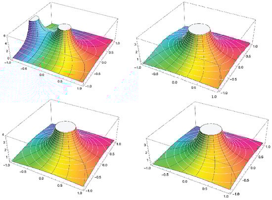
Figure 1. Complex 3D plot of ${\Gamma }_{\mathit{\ell }}\left(\xi \right),\xi =x+iy,\mathit{\ell }=1,2,3,4$ accordingly, where $z-$axis represents to ${\Gamma }_{\mathit{\ell }}\left(\xi \right)$.

• $\Gamma \left(\xi \right)={lim}_{\mathit{\ell }\to 1}{\Gamma }_{\mathit{\ell }}\left(\xi \right);$
• ${\Gamma }_{\mathit{\ell }}\left(\xi \right)={\mathit{\ell }}^{{\displaystyle \frac{\xi }{\mathit{\ell }}}-1}\Gamma \left({\displaystyle \frac{\xi }{\mathit{\ell }}}\right);$
• ${\Gamma }_{\mathit{\ell }}(\xi +\mathit{\ell })=\xi {\Gamma }_{\mathit{\ell }}\left(\xi \right);$
• ${\Gamma }_{\mathit{\ell }}(\mathit{\ell })=1.$

Definition 1

([1]). Assuming that $\vartheta \left(\xi \right)$ is differentiated over (0, b), the following is the corresponding value of the Caputo fractal–fractional derivative:

$${}^{\mathcal{C}}\mathcal{V}_{\xi }^{\mu ,\nu }\vartheta \left(\xi \right):={\displaystyle \frac{1}{\Gamma (n-\mu )}}{\int }_0^{\xi }{\displaystyle \frac{d\vartheta \left(t\right)}{d{t}^{\nu }}}{(\xi -t)}^{n-\mu -1}dt,\mu ,\nu \in (n-1,n].$$

Furthermore, the Riemann–Liouville fractal–fractional differential operator for a continuous function $\vartheta \left(\xi \right)$ that is fractal differentiable over (0, b) is as outlined below:

$${}^{\mathcal{RL}}\mathcal{V}_{\xi }^{\mu ,\nu }\vartheta \left(\xi \right):={\displaystyle \frac{1}{\Gamma (n-\mu )}}{\displaystyle \frac{d}{d{\xi }^{\nu }}}{\int }_0^{\xi }\vartheta \left(t\right){(\xi -t)}^{n-\mu -1}\mathrm{d}\mathrm{t},\mu ,\nu \in (n-1,n],$$

where

$${\displaystyle \frac{d\vartheta \left(\xi \right)}{d{\xi }^{\nu }}}=\underset{\xi \to t}{lim}{\displaystyle \frac{\vartheta \left(\xi \right)-\vartheta \left(t\right)}{{\xi }^{\nu }-t^{\nu }}}.$$

Considering those mentioned operators, further modification is developed with the following structure:

$${}^{\mathcal{C}}\mathcal{V}_{\xi }^{\mu ,\nu ,\gamma }\vartheta \left(\xi \right):={\displaystyle \frac{1}{\Gamma (n-\mu )}}{\int }_0^{\xi }{\displaystyle \frac{d^{\gamma }\vartheta \left(t\right)}{d{t}^{\nu }}}{(\xi -t)}^{n-\mu -1}\mathrm{d}\mathrm{t},\mu ,\nu ,\gamma \in (n-1,n].$$

And

$${}^{\mathcal{RL}}\mathcal{V}_{\xi }^{\mu ,\nu ,\gamma }\vartheta \left(\xi \right):={\displaystyle \frac{1}{\Gamma (n-\mu )}}{\displaystyle \frac{d^{\gamma }}{d{\xi }^{\nu }}}{\int }_0^{\xi }\vartheta \left(t\right){(\xi -t)}^{n-\mu -1}\mathrm{d}\mathrm{t},\mu ,\nu ,\gamma \in (n-1,n],$$

where

$${\displaystyle \frac{d^{\gamma }\vartheta \left(\xi \right)}{d{\xi }^{\nu }}}=\underset{\xi \to t}{lim}{\displaystyle \frac{{\vartheta }^{\gamma }\left(\xi \right)-{\vartheta }^{\gamma }\left(t\right)}{{\xi }^{\nu }-t^{\nu }}}.$$

Similarly, the arrangement formulates the fractal–fractional integral operator of order $\mu ,\nu >0$:

$${\mathsf{\Lambda }}_{\xi }^{\mu ,\nu }\vartheta \left(\xi \right):={\displaystyle \frac{\nu }{\Gamma \left(\mu \right)}}{\int }_0^{\xi }{t}^{\mu -1}\vartheta \left(t\right){(\xi -t)}^{\mu -1}\mathrm{d}\mathrm{t},\mu ,\nu >0.$$

The generalized fractal–fractional operators may be obtained by joining the specifications of the $\mathit{\ell }-$gamma function with the fractal–fractional operators, as shown below:

Definition 2.

Assume that the variable $\vartheta \left(\xi \right)$ is differentiable over the open interval from 0 to b. Next, the following is the Caputo $\mathit{\ell }-$fractal–fractional derivative:

$${}_{e}ll^{\mathcal{C}}{\mathcal{V}}_{\xi }^{\mu ,\nu }\vartheta \left(\xi \right):={\displaystyle \frac{1}{\mathit{\ell }{\Gamma }_{\mathit{\ell }}(n-\mu )}}{\int }_0^{\xi }{\displaystyle \frac{d\vartheta \left(t\right)}{d{t}^{\frac{\nu }{\mathit{\ell }}}}}{(\xi -t)}^{n-{\displaystyle \frac{\mu }{\mathit{\ell }}}-1}\mathrm{d}\mathrm{t},\mu ,\nu \in (n-1,n].$$

Additionally, the following expression provides the Riemann–Liouville $\mathit{\ell }-$fractal–fractional differential operator for a continuous function ϑ that is differentiated over (0, b):

$${}_{\mathit{\ell }\hspace{1em}}{}^{\mathcal{RL}}\mathcal{V}_{\xi }^{\mu ,\nu }\vartheta \left(\xi \right):={\displaystyle \frac{1}{\mathit{\ell }{\Gamma }_{\mathit{\ell }}(n-\mu )}}{\displaystyle \frac{d}{d{\xi }^{\frac{\nu }{\mathit{\ell }}}}}{\int }_0^{\chi }\vartheta \left(t\right){(\xi -t)}^{n-{\displaystyle \frac{\mu }{\mathit{\ell }}}-1}\mathrm{d}\mathrm{t},\mu ,\nu \in (n-1,n],$$

where

$${\displaystyle \frac{d\vartheta \left(\xi \right)}{d{\xi }^{\frac{\nu }{\mathit{\ell }}}}}=\underset{\xi \to t}{lim}{\displaystyle \frac{\vartheta \left(\xi \right)-\vartheta \left(t\right)}{{\xi }^{\frac{\nu }{\mathit{\ell }}}-t^{\frac{\nu }{\mathit{\ell }}}}}.$$

Regarding the above-mentioned operators, further abstraction is taken into account in the following manner:

$${}_{\mathit{\ell }}{}^{\mathcal{C}}\mathcal{V}_{\xi }^{\mu ,\nu ,\gamma }\vartheta \left(\xi \right):={\displaystyle \frac{1}{\mathit{\ell }{\Gamma }_{\mathit{\ell }}(n-\mu )}}{\int }_0^{\xi }{\displaystyle \frac{d^{\frac{\gamma }{\mathit{\ell }}}\phi \left(t\right)}{d{t}^{\frac{\nu }{\mathit{\ell }}}}}{(\xi -t)}^{n-{\displaystyle \frac{\mu }{\mathit{\ell }}}-1}\mathrm{d}\mathrm{t},\mu ,\nu ,\gamma \in (n-1,n].$$

And

$${}_{\mathit{\ell }\hspace{1em}}{}^{\mathcal{RL}}\mathcal{V}_{\xi }^{\mu ,\nu ,\gamma }\vartheta \left(\xi \right):={\displaystyle \frac{1}{\mathit{\ell }{\Gamma }_{\mathit{\ell }}(n-\mu )}}{\displaystyle \frac{d^{\frac{\gamma }{\mathit{\ell }}}}{d{\xi }^{\frac{\nu }{\mathit{\ell }}}}}{\int }_0^{\chi }\vartheta \left(t\right){(\xi -t)}^{n-{\displaystyle \frac{\mu }{\mathit{\ell }}}-1}\mathrm{d}\mathrm{t},\mu ,\nu ,\gamma \in (n-1,n],$$

where

$${\displaystyle \frac{d^{\frac{\gamma }{\mathit{\ell }}}\vartheta \left(\xi \right)}{d{\xi }^{\frac{\nu }{\mathit{\ell }}}}}=\underset{\chi \to t}{lim}{\displaystyle \frac{{\vartheta }^{\frac{\gamma }{\mathit{\ell }}}\left(\xi \right)-{\vartheta }^{\frac{\gamma }{\mathit{\ell }}}\left(t\right)}{{\xi }^{\frac{\nu }{\mathit{\ell }}}-t^{\frac{\nu }{\mathit{\ell }}}}}.$$

In accordance with this, the layout formulates the $\mathit{\ell }-$fractal–fractional integral operator of order $\mu ,\nu >0$:

$${}_{\mathit{\ell }}\mathsf{\Lambda }_{\xi }^{\mu ,\nu }\vartheta \left(\xi \right):={\displaystyle \frac{\nu }{\mathit{\ell }{\Gamma }_{\mathit{\ell }}\left(\mu \right)}}{\int }_0^{\xi }{t}^{{\displaystyle \frac{\mu }{\mathit{\ell }}}-1}\vartheta \left(t\right){(\xi -\tau )}^{{\displaystyle \frac{\mu }{\mathit{\ell }}}-1}\mathrm{d}\mathrm{t},\mu ,\nu >0.$$

Take note of that

$${\Gamma }_{\mathit{\ell }}\left(\mu \right)={\mathit{\ell }}^{{\displaystyle \frac{\mu }{\mathit{\ell }}}-1}\Gamma \left({\displaystyle \frac{\mu }{\mathit{\ell }}}\right).$$

Some examples are given in the next subsection.

2. Illustrations of $\mathsf{\ell }\mathbf{-}$Fractal–Fractional Operator

Example 1.

Let $\vartheta \left(\xi \right)={\xi }^m$ (see [10])

As

$${\displaystyle \frac{d\vartheta \left(\xi \right)}{d{\xi }^{\nu }}}=\underset{\xi \to t}{lim}{\displaystyle \frac{{\xi }^m-t^m}{{\xi }^{\nu }-t^{\nu }}}={\displaystyle \frac{m{t}^{m-\nu }}{\nu }}$$

this provides

$$\begin{array}{cc}\hfill {}^{\mathcal{C}}\mathcal{V}_{\xi }^{\mu ,\nu }{\xi }^m& ={\displaystyle \frac{m}{\nu \Gamma (1-\mu )}}{\int }_0^{\xi }\left(t^{m-\nu }\right){(\xi -t)}^{-\mu }\mathrm{d}\mathrm{t},\mu ,\nu \in (0,1]\hfill \\ \hfill & ={\displaystyle \frac{m}{\nu \Gamma (1-\mu )}}{\displaystyle \frac{\Gamma (m-\nu +1)\Gamma (1-\mu ){\xi }^{m-\nu -\mu +1}}{\Gamma (m-\nu -\mu +2)}}\hfill \\ \hfill & =\left({\displaystyle \frac{m}{\nu }}{\displaystyle \frac{\Gamma (m-\nu +1)}{\Gamma (m-\nu -\mu +2)}}\right){\xi }^{m-\nu -\mu +1};\hfill \end{array}$$

and

$$\begin{array}{cc}\hfill {}^{\mathcal{RL}}\mathcal{V}_{\xi }^{\mu ,\nu }\left({\xi }^m\right)& ={\displaystyle \frac{1}{\Gamma (1-\mu )}}{\displaystyle \frac{d}{d{\xi }^{\nu }}}{\int }_0^{\xi }\left(t^m\right){(\xi -t)}^{-\mu }\mathrm{d}\mathrm{t},\mu ,\nu \in (0,1]\hfill \\ \hfill & ={\displaystyle \frac{1}{\Gamma (1-\mu )}}{\displaystyle \frac{d}{d{\xi }^{\nu }}}\left({\displaystyle \frac{\Gamma (m+1)\Gamma (1-\mu ){\xi }^{m-\mu +1}}{\Gamma (m-\mu +2)}}\right)\hfill \\ \hfill & ={\displaystyle \frac{1}{\Gamma (1-\mu )}}\left({\displaystyle \frac{\Gamma (m+1)\Gamma (1-\mu )}{\Gamma (m-\mu +2)}}\right)\left({\displaystyle \frac{d}{d{\xi }^{\nu }}}{\xi }^{m-\mu +1}\right).\hfill \end{array}$$

But

$$\left({\displaystyle \frac{d}{d{\xi }^{\nu }}}{\xi }^{m-\mu +1}\right)={\displaystyle \frac{(-\mu +m+1){\xi }^{-\mu +m-\nu +1}}{\nu }}$$

thus, we obtain

$$\begin{array}{cc}\hfill {}^{\mathcal{RL}}\mathcal{V}_{\xi }^{\mu ,\nu }\left({\xi }^m\right)& =\left({\displaystyle \frac{\Gamma (m+1)\Gamma (1-\mu )}{\Gamma (m-\mu +2)}}\right)\left({\displaystyle \frac{(-\mu +m+1){\xi }^{-\mu +m-\nu +1}}{\nu \Gamma (1-\mu )}}\right)\hfill \\ \hfill & =\left({\displaystyle \frac{\Gamma (m+1)}{\Gamma (m-\mu +2)}}\right)\left({\displaystyle \frac{m+1-\mu }{\nu }}\right){\xi }^{-\mu +m-\nu +1}.\hfill \end{array}$$

The integral of ϑ yields

$$\begin{array}{cc}\hfill {\mathsf{\Lambda }}_{\xi }^{\mu ,\nu }{\xi }^m& ={\displaystyle \frac{\nu }{\Gamma \left(\mu \right)}}{\int }_0^{\xi }{t}^{\mu -1}{t}^m{(\xi -\tau )}^{\mu -1}\mathrm{d}\mathrm{t},\hfill \\ \hfill & ={\displaystyle \frac{\nu }{\Gamma \left(\mu \right)}}{\int }_0^{\xi }{t}^{\mu -1+m}{(\xi -\tau )}^{\mu -1}\mathrm{d}\mathrm{t},\hfill \\ \hfill & ={\displaystyle \frac{\nu }{\Gamma \left(\mu \right)}}{\displaystyle \frac{\Gamma (\mu -1+m+1)\Gamma \left(\mu \right){\xi }^{\mu -1+m+\mu }}{\Gamma (\mu -1+m+\mu +1)}}\hfill \\ \hfill & ={\displaystyle \frac{\nu \Gamma (\mu +m){\xi }^{2\mu -1+m}}{\Gamma (2\mu +m)}}.\hfill \end{array}$$

By using the fact

$${\displaystyle \frac{d^{\gamma }\vartheta \left(\xi \right)}{d{\xi }^{\nu }}}=\underset{\xi \to t}{lim}{\displaystyle \frac{{\xi }^{\gamma m}-t^{\gamma m}}{{\xi }^{\nu }-t^{\nu }}}={\displaystyle \frac{\gamma m{t}^{\gamma m-\nu }}{\nu }},$$

we obtain the next derivative

$$\begin{array}{cc}\hfill {}^{\mathcal{C}}\mathcal{V}_{\xi }^{\mu ,\nu ,\gamma }\left({\xi }^m\right)& ={\displaystyle \frac{\gamma m}{\nu \Gamma (1-\mu )}}{\int }_0^{\xi }\left(t^{\gamma m-\nu }\right){(\xi -t)}^{-\mu }\mathrm{d}\mathrm{t},\mu ,\nu ,\gamma \in (0,1]\hfill \\ \hfill & ={\displaystyle \frac{\gamma m}{\nu \Gamma (1-\mu )}}\left({\displaystyle \frac{\Gamma (1-\mu )\Gamma (\gamma m-\nu +1){\xi }^{\gamma m-\mu -\nu +1}}{\Gamma (\gamma m-\mu -\nu +2)}}\right)\hfill \\ \hfill & ={\displaystyle \frac{\gamma m}{\nu }}\left({\displaystyle \frac{\Gamma (\gamma m-\nu +1){\xi }^{\gamma m-\mu -\nu +1}}{\Gamma (\gamma m-\mu -\nu +2)}}\right).\hfill \end{array}$$

Additionally, we obtain

$$\begin{array}{cc}\hfill {}^{\mathcal{RL}}\mathcal{V}_{\xi }^{\mu ,\nu ,\gamma }\left({\xi }^m\right)& ={\displaystyle \frac{1}{\Gamma (1-\mu )}}{\displaystyle \frac{d^{\gamma }}{d{\xi }^{\nu }}}{\int }_0^{\xi }\left(t^m\right){(\xi -t)}^{-\mu }\mathrm{d}\mathrm{t},\mu ,\nu ,\gamma \in (0,1]\hfill \\ \hfill & ={\displaystyle \frac{1}{\Gamma (1-\mu )}}{\displaystyle \frac{d^{\gamma }}{d{\xi }^{\nu }}}\left({\displaystyle \frac{\Gamma (m+1)\Gamma (1-\mu ){\xi }^{m-\mu +1}}{\Gamma (m-\mu +2)}}\right)\hfill \\ \hfill & =\left({\displaystyle \frac{\Gamma (m+1)}{\Gamma (m-\mu +2)}}\right)\left({\displaystyle \frac{\gamma (-\mu +m+1)}{\nu }}\right){\xi }^{\gamma (-\mu +m+1)-\nu }.\hfill \end{array}$$

Example 2.

Currently, we have the extended ℓ-fractal–fractional operators:

$${\displaystyle \frac{d\vartheta \left(\xi \right)}{d{\xi }^{\nu }}}=\underset{\xi \to t}{lim}{\displaystyle \frac{{\xi }^m-t^m}{{\xi }^{\frac{\nu }{\mathit{\ell }}}-t^{\frac{\nu }{\mathit{\ell }}}}}={\displaystyle \frac{m\mathit{\ell }{t}^{m-\frac{\nu }{\mathit{\ell }}}}{\nu }}$$

then

$$\begin{array}{cc}\hfill {}_{\mathit{\ell }}{}^{\mathcal{C}}\mathcal{V}_{\xi }^{\mu ,\nu }{\xi }^m& ={\displaystyle \frac{m\mathit{\ell }}{\nu \mathit{\ell }{\Gamma }_{\mathit{\ell }}(1-\mu )}}{\int }_0^{\xi }\left(t^{m-{\displaystyle \frac{\nu }{\mathit{\ell }}}}\right){(\xi -t)}^{-{\displaystyle \frac{\mu }{\mathit{\ell }}}}\mathrm{d}\mathrm{t},\mu ,\nu \in (0,1]\hfill \\ \hfill & ={\displaystyle \frac{m}{\nu {\Gamma }_{\mathit{\ell }}(1-\mu )}}{\displaystyle \frac{\Gamma \left(1-\frac{\mu }{\mathit{\ell }}\right)\Gamma \left(m-\frac{\nu }{\mathit{\ell }}+1\right){\xi }^{\frac{m\mathit{\ell }+\mathit{\ell }-\mu -\nu }{\mathit{\ell }}}}{\Gamma \left(m-\frac{-2\mathit{\ell }+\mu +\nu }{\mathit{\ell }}\right)}}.\hfill \end{array}$$

$$\begin{array}{cc}\hfill {}_{p\hspace{1em}}{}^{\mathcal{RL}}\mathcal{V}_{\xi }^{\mu ,\nu }\left({\xi }^m\right)& ={\displaystyle \frac{1}{\mathit{\ell }{\Gamma }_{\mathit{\ell }}(1-\mu )}}{\displaystyle \frac{d}{d{\xi }^{\frac{\nu }{\mathit{\ell }}}}}{\int }_0^{\xi }\left(t^m\right){(\xi -t)}^{-{\displaystyle \frac{\mu }{\mathit{\ell }}}}\mathrm{d}\mathrm{t},\mu ,\nu \in (0,1]\hfill \\ \hfill & ={\displaystyle \frac{1}{\mathit{\ell }{\Gamma }_{\mathit{\ell }}(1-\mu )}}{\displaystyle \frac{d}{d{\xi }^{\frac{\nu }{\mathit{\ell }}}}}\left({\displaystyle \frac{\Gamma (m+1)\Gamma \left(1-\frac{\mu }{\mathit{\ell }}\right){\xi }^{m-\frac{\mu }{\mathit{\ell }}+1}}{\Gamma \left(m-\frac{\mu }{\mathit{\ell }}+2\right)}}\right)\hfill \\ \hfill & ={\displaystyle \frac{1}{\mathit{\ell }{\Gamma }_{\mathit{\ell }}(1-\mu )}}\left({\displaystyle \frac{\Gamma (m+1)\Gamma (1-\frac{\mu }{\mathit{\ell }})}{\Gamma (m-\frac{\mu }{\mathit{\ell }}+2)}}\right)\left({\displaystyle \frac{d}{d{\xi }^{\frac{\nu }{\mathit{\ell }}}}}{\chi }^{m-{\displaystyle \frac{\mu }{\mathit{\ell }}}+1}\right).\hfill \end{array}$$

By utilizing the derivative

$$\left({\displaystyle \frac{d}{d{\xi }^{\frac{\nu }{\mathit{\ell }}}}}{\xi }^{m-{\displaystyle \frac{\mu }{\mathit{\ell }}}+1}\right)=\left({\displaystyle \frac{-\mu +m\mathit{\ell }+\mathit{\ell }}{\nu }}\right){\xi }^{{\displaystyle \frac{(-\mu +m\mathit{\ell }+\mathit{\ell }-\nu )}{\mathit{\ell }}}}$$

we obtain

$$\begin{array}{cc}\hfill {}_{\mathit{\ell }\hspace{1em}}{}^{\mathcal{RL}}\mathcal{V}_{\xi }^{\mu ,\nu }\left({\xi }^m\right)& =\left({\displaystyle \frac{(m-\mu \mathit{\ell }+\mathit{\ell })}{\nu \mathit{\ell }{\Gamma }_{\mathit{\ell }}(1-\mu )}}\right)\left({\displaystyle \frac{\Gamma (m+1)\Gamma (1-\frac{\mu }{\mathit{\ell }})}{\Gamma (m-\frac{\mu }{\mathit{\ell }}+2)}}\right){\xi }^{{\displaystyle \frac{m\mathit{\ell }+\mathit{\ell }-\nu -\mu }{\mathit{\ell }}}}.\hfill \end{array}$$

The $\mathit{\ell }-$fractal–fractional integral indicates that

$$\begin{array}{cc}\hfill {}_{\mathit{\ell }}\mathsf{\Lambda }_{\xi }^{\mu ,\nu }{\xi }^m& ={\displaystyle \frac{\nu }{\mathit{\ell }{\Gamma }_{\mathit{\ell }}\left(\mu \right)}}{\int }_0^{\xi }{t}^{{\displaystyle \frac{\mu }{\mathit{\ell }}}-1}{t}^m{(\xi -t)}^{{\displaystyle \frac{\mu }{\mathit{\ell }}}-1}\mathrm{d}\mathrm{t},\hfill \\ \hfill & ={\displaystyle \frac{\nu }{\mathit{\ell }{\Gamma }_{\mathit{\ell }}\left(\mu \right)}}{\int }_0^{\xi }{t}^{{\displaystyle \frac{\mu }{\mathit{\ell }}}-1+m}{(\xi -t)}^{{\displaystyle \frac{\mu }{\mathit{\ell }}}-1}\mathrm{d}\mathrm{t},\hfill \\ \hfill & ={\displaystyle \frac{\nu }{\mathit{\ell }{\Gamma }_{\mathit{\ell }}\left(\mu \right)}}{\displaystyle \frac{\Gamma \left(\frac{\mu }{\mathit{\ell }}\right){\xi }^{m+\frac{2\mu }{\mathit{\ell }}-1}\Gamma \left(m+\frac{\mu }{\mathit{\ell }}\right)}{\Gamma \left(m+\frac{2\mu }{\mathit{\ell }}\right)}}\hfill \\ \hfill & ={\displaystyle \frac{\nu }{\mathit{\ell }{\Gamma }_{\mathit{\ell }}\left(\mu \right)}}{\displaystyle \frac{{\mathit{\ell }}^{\frac{\mu }{\mathit{\ell }}-1}\Gamma \left(\frac{\mu }{\mathit{\ell }}\right){\xi }^{m+\frac{2\mu }{\mathit{\ell }}-1}\Gamma \left(m+\frac{\mu }{\mathit{\ell }}\right)}{{\mathit{\ell }}^{\frac{\mu }{\mathit{\ell }}-1}\Gamma \left(m+\frac{2\mu }{p}\right)}}\hfill \\ \hfill & =\left({\displaystyle \frac{\nu \Gamma \left(m+\frac{\mu }{\mathit{\ell }}\right)}{{\mathit{\ell }}^{\frac{\mu }{\mathit{\ell }}-1}\Gamma \left(m+\frac{2\mu }{\mathit{\ell }}\right)}}\right){\xi }^{m+{\displaystyle \frac{2\mu }{\mathit{\ell }}}-1}.\hfill \end{array}$$

By considering the derivative

$${\displaystyle \frac{d^{\frac{\gamma }{\mathit{\ell }}}\vartheta \left(\xi \right)}{d{\xi }^{\frac{\nu }{\mathit{\ell }}}}}=\underset{\xi \to t}{lim}{\displaystyle \frac{{\xi }^{\left(\frac{\gamma }{\mathit{\ell }}\right)m}-t^{\left(\frac{\gamma }{\mathit{\ell }}\right)m}}{{\xi }^{\frac{\nu }{\mathit{\ell }}}-t^{\frac{\nu }{\mathit{\ell }}}}}=\left({\displaystyle \frac{\gamma m}{\nu }}\right)t^{{\displaystyle \frac{(\gamma m-\nu )}{\mathit{\ell }}}},$$

one can obtain

$$\begin{array}{cc}\hfill {}_{\mathit{\ell }}{}^{\mathcal{C}}\mathcal{V}_{\xi }^{\mu ,\nu ,\gamma }\left({\xi }^m\right)& ={\displaystyle \frac{\gamma m}{\nu {\mathit{\ell }}^{(1-\mu )/\mathit{\ell }}\Gamma \left({\displaystyle \frac{1-\mu }{\mathit{\ell }}}\right)}}{\int }_0^{\chi }\left(t^{(\gamma m-\nu )/\mathit{\ell }}\right){(\xi -t)}^{-\mu /\mathit{\ell }}\mathrm{d}\mathrm{t},\mu ,\nu ,\gamma \in (0,1]\hfill \\ \hfill & ={\displaystyle \frac{\gamma m}{\nu {\mathit{\ell }}^{(1-\mu )/\mathit{\ell }}}}\left({\displaystyle \frac{\Gamma (1-{\displaystyle \frac{\mu }{\mathit{\ell }}})\Gamma \left(\frac{\gamma m+\mathit{\ell }-\nu }{\mathit{\ell }}\right){\xi }^{\frac{\gamma m-\mu +\mathit{\ell }-\nu }{\mathit{\ell }}}}{\Gamma \left({\displaystyle \frac{1-\mu }{\mathit{\ell }}}\right)\Gamma \left(-\frac{-\gamma m-2\mathit{\ell }+\nu +\mu }{\mathit{\ell }}\right)}}\right)\hfill \\ \hfill & ={\displaystyle \frac{\gamma m}{\nu {\mathit{\ell }}^{(1-\mu )/\mathit{\ell }}}}\left({\displaystyle \frac{\Gamma (1-{\displaystyle \frac{\mu }{\mathit{\ell }}})\Gamma \left(\frac{\gamma m+\mathit{\ell }-\nu }{\mathit{\ell }}\right){\xi }^{\frac{\gamma m-\mu +\mathit{\ell }-\nu }{\mathit{\ell }}}}{\Gamma \left({\displaystyle \frac{1-\mu }{\mathit{\ell }}}\right)\Gamma \left(-\frac{-\gamma m-2\mathit{\ell }+\nu +\mu }{\mathit{\ell }}\right)}}\right).\hfill \end{array}$$

Also, we obtain

$$\begin{array}{cc}\hfill {}_{\mathit{\ell }\hspace{1em}}{}^{\mathcal{RL}}\mathcal{V}_{\xi }^{\mu ,\nu ,\gamma }\left({\xi }^m\right)& ={\displaystyle \frac{1}{{\mathit{\ell }}^{(1-\mu )/\mathit{\ell }}\Gamma \left({\displaystyle \frac{1-\mu }{\mathit{\ell }}}\right)}}{\displaystyle \frac{d^{\gamma /\mathit{\ell }}}{d{\xi }^{\nu /\mathit{\ell }}}}{\int }_0^{\xi }\left(t^m\right){(\xi -t)}^{-\mu /\mathit{\ell }}\mathrm{d}\mathrm{t},\mu ,\nu ,\gamma \in (0,1]\hfill \\ \hfill & ={\displaystyle \frac{1}{{\mathit{\ell }}^{(1-\mu )/\mathit{\ell }}\Gamma \left({\displaystyle \frac{1-\mu }{\mathit{\ell }}}\right)}}{\displaystyle \frac{d^{\gamma /\mathit{\ell }}}{d{\xi }^{\nu /\mathit{\ell }}}}\left({\displaystyle \frac{\Gamma (m+1)\Gamma (1-\mu /\mathit{\ell }){\xi }^{m-\mu /\mathit{\ell }+1}}{\Gamma (m-\mu /\mathit{\ell }+2)}}\right)\hfill \\ \hfill & ={\displaystyle \frac{\gamma \left(\mathit{\ell }+m\mathit{\ell }-\mu \right)}{\nu {\mathit{\ell }}^{(1-\mu )/\mathit{\ell }+1}}}\left({\displaystyle \frac{\Gamma (m+1)\Gamma (1-\mu /\mathit{\ell })}{\Gamma \left({\displaystyle \frac{1-\mu }{\mathit{\ell }}}\right)\Gamma (m-\mu /\mathit{\ell }+2)}}{\xi }^{-(\mathit{\ell }(\nu -(1+m)\gamma )+\gamma \mu )/{\mathit{\ell }}^2}\right).\hfill \end{array}$$

3. Complex Fractal–Fractional Operators

Definition 2 for a complex variable, $\mathit{\ell }-$fractal–fractional operators can be constructed. Initial, we propose acting on a class of analytic functions of the framework using the $\mathit{\ell }-$operators.

$$\sigma \left(\xi \right)=\xi +\sum _{n=2}^{\infty }{\sigma }_n{\xi }^n,\xi \in \mathbb{O}:=\{\xi \in \mathbb{C}:|\xi |<1\}.$$

(1)

The normalization class of analytic functions in $\mathbb{O}$ fulfilling $\sigma \left(0\right)=0,{\sigma }^{\prime }\left(0\right)=1$ is the name given to this class. We are able to analyze it analytically thanks to this type of analytic function.

Definition 3.

Suppose that in $\mathbb{O}$, σ is analytic. Next, the following is the Caputo $\mathit{\ell }-$fractal–fractional differential operator:

$${}_{\mathit{\ell }}{}^{\mathcal{C}}\mathcal{V}_{\xi }^{\mu ,\nu }\sigma \left(\xi \right):={\displaystyle \frac{1}{\mathit{\ell }{\Gamma }_{\mathit{\ell }}(n-\mu )}}{\int }_0^{\xi }{\displaystyle \frac{d\sigma \left(z\right)}{d{z}^{\frac{\nu }{\mathit{\ell }}}}}{(\xi -z)}^{n-{\displaystyle \frac{\mu }{\mathit{\ell }}}-1}dz,\mu ,\nu \in (n-1,n].$$

Additionally, the Riemann–Liouville $\mathit{\ell }-$fractal–fractional differential operator is provided by the following expression if the function is a fractal analytic function in $\mathbb{O}$:

$${}_{\mathit{\ell }\hspace{1em}}{}^{\mathcal{RL}}\mathcal{V}_{\xi }^{\mu ,\nu }\sigma \left(\xi \right):={\displaystyle \frac{1}{\mathit{\ell }{\Gamma }_{\mathit{\ell }}(n-\mu )}}{\displaystyle \frac{d}{d{\xi }^{\frac{\nu }{\mathit{\ell }}}}}{\int }_0^{\xi }\sigma \left(z\right){(\xi -z)}^{n-{\displaystyle \frac{\mu }{\mathit{\ell }}}-1}dz,\mu ,\nu \in (n-1,n],$$

where

$${\displaystyle \frac{d\sigma \left(\xi \right)}{d{\xi }^{\frac{\nu }{\mathit{\ell }}}}}=\underset{\xi \to z}{lim}{\displaystyle \frac{\sigma \left(\xi \right)-\sigma \left(z\right)}{{\xi }^{\frac{\nu }{\mathit{\ell }}}-z^{\frac{\nu }{\mathit{\ell }}}}}.$$

For the above-mentioned operators, further expansion is expected in the following ways:

$${}_{\mathit{\ell }}{}^{\mathcal{C}}\mathcal{V}_{\xi }^{\mu ,\nu ,\gamma }\varphi \left(z\right):={\displaystyle \frac{1}{\mathit{\ell }{\Gamma }_{\mathit{\ell }}(n-\mu )}}{\int }_0^z{\displaystyle \frac{d^{\gamma /\mathit{\ell }}\varphi \left(\zeta \right)}{d{\zeta }^{\nu /\mathit{\ell }}}}{(z-\zeta )}^{n-\mu /\mathit{\ell }-1}d\zeta ,\mu ,\nu ,\gamma \in (n-1,n].$$

And

$${}_{\mathit{\ell }\hspace{1em}}{}^{\mathcal{RL}}\mathcal{V}_{\xi }^{\mu ,\nu ,\gamma }\sigma \left(\xi \right):={\displaystyle \frac{1}{\mathit{\ell }{\Gamma }_{\mathit{\ell }}(n-\mu )}}{\displaystyle \frac{d^{\gamma /\mathit{\ell }}}{d{z}^{\nu /\mathit{\ell }}}}{\int }_0^{\xi }\sigma \left(z\right){(\xi -z)}^{n-{\displaystyle \frac{\mu }{\mathit{\ell }}}-1}dz,\mu ,\nu ,\gamma \in (n-1,n],$$

where

$${\displaystyle \frac{d^{\frac{\gamma }{\mathit{\ell }}}\sigma \left(\xi \right)}{d{\xi }^{\frac{\nu }{\mathit{\ell }}}}}=\underset{\xi \to z}{lim}{\displaystyle \frac{{\sigma }^{\frac{\gamma }{\mathit{\ell }}}\left(\xi \right)-{\sigma }^{\frac{\gamma }{\mathit{\ell }}}\left(z\right)}{{\xi }^{\frac{\nu }{\mathit{\ell }}}-z^{\frac{\nu }{\mathit{\ell }}}}},\xi ,z\in \mathbb{O}.$$

In accordance with this, the layout formulates the $\mathit{\ell }-$fractal–fractional integral operator of order $\mu ,\nu >0$:

$${}_{\mathit{\ell }}\mathsf{\Lambda }_{\xi }^{\mu ,\nu }\sigma \left(\xi \right):={\displaystyle \frac{\nu }{\mathit{\ell }{\Gamma }_{\mathit{\ell }}\left(\mu \right)}}{\int }_0^{\xi }{z}^{{\displaystyle \frac{\mu }{\mathit{\ell }}}-1}\sigma \left(z\right){(\xi -z)}^{{\displaystyle \frac{\mu }{\mathit{\ell }}}-1}dz,\mu ,\nu >0,z,\xi \in \mathbb{O},$$

where

$${\Gamma }_{\mathit{\ell }}\left(\mu \right)={\mathit{\ell }}^{{\displaystyle \frac{\mu }{\mathit{\ell }}}-1}\Gamma \left({\displaystyle \frac{\mu }{\mathit{\ell }}}\right).$$

Example 3.

Suppose the analytic function σ, with the expansion in (1). We have the subsequent information:

$$\begin{array}{cc}\hfill {}_{\mathit{\ell }}{}^{\mathcal{C}}\mathcal{V}_{\xi }^{\mu ,\nu }\sigma \left(\xi \right)& ={}_{\mathit{\ell }}{}^{\mathcal{C}}\mathcal{V}_{\xi }^{\mu ,\nu }\left(\xi +\sum _{n=2}^{\infty }{\sigma }_n{\xi }^n\right)\hfill \\ \hfill & ={}_{\mathit{\ell }}{}^{\mathcal{C}}\mathcal{V}_{\xi }^{\mu ,\nu }\xi +\sum _{n=2}^{\infty }{\sigma }_n{}_{\mathit{\ell }}{}^{\mathcal{C}}\mathcal{V}_{\xi }^{\mu ,\nu }{\xi }^n\hfill \\ \hfill & ={\displaystyle \frac{1}{\nu {\Gamma }_{\mathit{\ell }}(1-\mu )}}{\displaystyle \frac{\Gamma \left(1-\frac{\mu }{\mathit{\ell }}\right)\Gamma \left(1-\frac{\nu }{\mathit{\ell }}+1\right){\xi }^{\frac{2\mathit{\ell }-\mu -\nu }{\mathit{\ell }}}}{\Gamma \left(1-\frac{-2\mathit{\ell }+\mu +\nu }{\mathit{\ell }}\right)}}\hfill \\ \hfill & +\sum _{n=2}^{\infty }{\sigma }_n{\displaystyle \frac{n}{\nu {\Gamma }_{\mathit{\ell }}(1-\mu )}}{\displaystyle \frac{\Gamma \left(1-\frac{\mu }{\mathit{\ell }}\right)\Gamma \left(n-\frac{\nu }{\mathit{\ell }}+1\right){\xi }^{\frac{n\mathit{\ell }+\mathit{\ell }-\mu -\nu }{\mathit{\ell }}}}{\Gamma \left(n-\frac{-2\mathit{\ell }+\mu +\nu }{\mathit{\ell }}\right)}}\hfill \\ \hfill & ={\displaystyle \frac{1}{\nu {\mathit{\ell }}^{\frac{1-\mu }{\mathit{\ell }}-1}\Gamma \left(\frac{1-\mu }{\mathit{\ell }}\right)}}{\displaystyle \frac{\Gamma \left(1-\frac{\mu }{\mathit{\ell }}\right)\Gamma \left(1-\frac{\nu }{\mathit{\ell }}+1\right){\xi }^{\frac{2\mathit{\ell }-\mu -\nu }{\mathit{\ell }}}}{\Gamma \left(1-\frac{-2\mathit{\ell }+\mu +\nu }{\mathit{\ell }}\right)}}\hfill \\ \hfill & +\sum _{n=2}^{\infty }{\sigma }_n{\displaystyle \frac{n}{\nu {\mathit{\ell }}^{\frac{1-\mu }{\mathit{\ell }}-1}\Gamma \left(\frac{1-\mu }{\mathit{\ell }}\right)}}{\displaystyle \frac{\Gamma \left(1-\frac{\mu }{\mathit{\ell }}\right)\Gamma \left(n-\frac{\nu }{\mathit{\ell }}+1\right){\xi }^{\frac{n\mathit{\ell }+\mathit{\ell }-\mu -\nu }{\mathit{\ell }}}}{\Gamma \left(n-\frac{-2\mathit{\ell }+\mu +\nu }{\mathit{\ell }}\right)}}.\hfill \end{array}$$

In addition, we obtain the following computation:

$$\begin{array}{cc}\hfill {}_{\mathit{\ell }}{}^{\mathcal{RL}}\mathcal{V}_{\xi }^{\mu ,\nu }\sigma \left(\xi \right)& ={}_{\mathit{\ell }}{}^{\mathcal{RL}}\mathcal{V}_{\xi }^{\mu ,\nu }\left(\xi \right)+\sum _{n=2}^{\infty }{\sigma }_n{}_{\mathit{\ell }}{}^{\mathcal{RL}}\mathcal{V}_{\xi }^{\mu ,\nu }{\xi }^n\hfill \\ \hfill & ={\displaystyle \frac{1}{{\mathit{\ell }}^{\frac{1-\mu }{\mathit{\ell }}}\Gamma \left(\frac{1-\mu }{\mathit{\ell }}\right)}}\left({\displaystyle \frac{\Gamma (1-\mu /\mathit{\ell })}{\Gamma (3-\mu /\mathit{\ell })}}\right){\displaystyle \frac{(-\mu +2\mathit{\ell }){\xi }^{(-\mu +2\mathit{\ell }-\nu )/\mathit{\ell }}}{\nu }}\hfill \\ \hfill & +\left({\displaystyle \frac{1}{{\mathit{\ell }}^{\frac{1-\mu }{\mathit{\ell }}}\Gamma \left(\frac{1-\mu }{\mathit{\ell }}\right)}}\right)\sum _{n=2}^{\infty }{\sigma }_n\left({\displaystyle \frac{\Gamma (n+1)\Gamma (1-\mu \mathit{\ell })}{\Gamma (n-\mu /\mathit{\ell }+2)}}\right)\hfill \\ \hfill & \times \left({\displaystyle \frac{(-\mu +n\mathit{\ell }+\mathit{\ell }){\xi }^{(-\mu +n\mathit{\ell }+\mathit{\ell }-\nu )/\mathit{\ell }}}{\nu }}\right).\hfill \end{array}$$

For the integral, we obtain the next evaluation

$$\begin{array}{cc}\hfill {}_{\mathit{\ell }}\mathsf{\Lambda }_{\xi }^{\mu ,\nu }\sigma \left(\xi \right)& ={}_{\mathit{\ell }}\mathsf{\Lambda }_{\xi }^{\mu ,\nu }\left(\xi \right)+\sum _{n=2}^{\infty }{\sigma }_n{}_{\mathit{\ell }}\mathsf{\Lambda }_{\xi }^{\mu ,\nu }{\xi }^n\hfill \\ \hfill & =\left({\displaystyle \frac{\nu \Gamma \left(1+\frac{\mu }{\mathit{\ell }}\right)}{{\mathit{\ell }}^{\frac{\mu }{\mathit{\ell }}-1}\Gamma \left(1+\frac{2\mu }{\mathit{\ell }}\right)}}\right){\xi }^{{\displaystyle \frac{2\mu }{\mathit{\ell }}}}+\sum _{n=2}^{\infty }{\sigma }_n\left({\displaystyle \frac{\nu \Gamma \left(n+\frac{\mu }{\mathit{\ell }}\right)}{{\mathit{\ell }}^{\frac{\mu }{\mathit{\ell }}-1}\Gamma \left(n+\frac{2\mu }{\mathit{\ell }}\right)}}\right){\xi }^{n+{\displaystyle \frac{2\mu }{\mathit{\ell }}}-1}.\hfill \end{array}$$

As an example, we possess the triple parametric $\mathit{\ell }-$fractal–fractional operator

$$\begin{array}{cc}\hfill {}_{\mathit{\ell }}{}^{\mathcal{C}}\mathcal{V}_{\xi }^{\mu ,\nu ,\gamma }\sigma \left(\xi \right)& ={\displaystyle \frac{\gamma }{\nu {\mathit{\ell }}^{(1-\mu )/\mathit{\ell }}}}\left({\displaystyle \frac{\Gamma (1-{\displaystyle \frac{\mu }{\mathit{\ell }}})\Gamma \left(\frac{\gamma +\mathit{\ell }-\nu }{\mathit{\ell }}\right){\xi }^{\frac{\gamma -\mu +\mathit{\ell }-\nu }{\mathit{\ell }}}}{\Gamma \left({\displaystyle \frac{1-\mu }{\mathit{\ell }}}\right)\Gamma \left(-\frac{-\gamma -2\mathit{\ell }+\nu +\mu }{\mathit{\ell }}\right)}}\right)\hfill \\ \hfill & +\sum _{n=2}^{\infty }{\sigma }_n{\displaystyle \frac{\gamma n}{\nu {\mathit{\ell }}^{(1-\mu )/\mathit{\ell }}}}\left({\displaystyle \frac{\Gamma (1-{\displaystyle \frac{\mu }{\mathit{\ell }}})\Gamma \left(\frac{\gamma n+\mathit{\ell }-\nu }{\mathit{\ell }}\right){\xi }^{\frac{\gamma n-\mu +\mathit{\ell }-\nu }{\mathit{\ell }}}}{\Gamma \left({\displaystyle \frac{1-\mu }{\mathit{\ell }}}\right)\Gamma \left(-\frac{\nu +\mu -\gamma n-2\mathit{\ell }}{\mathit{\ell }}\right)}}\right).\hfill \end{array}$$

Moreover, we obtain

$$\begin{array}{cc}\hfill {}_{\mathit{\ell }\hspace{1em}}{}^{\mathcal{RL}}\mathcal{V}_{\xi }^{\mu ,\nu ,\gamma }\sigma \left(\xi \right)& ={\displaystyle \frac{\gamma \left(\mathit{\ell }+\mathit{\ell }-\mu \right)}{\nu {\mathit{\ell }}^{(1-\mu )/\mathit{\ell }+1}}}\left({\displaystyle \frac{\Gamma \left(2\right)\Gamma (1-\mu /\mathit{\ell })}{\Gamma \left({\displaystyle \frac{1-\mu }{\mathit{\ell }}}\right)\Gamma (3-\mu /\mathit{\ell })}}{\xi }^{-(\mathit{\ell }(\nu -2\gamma )+\gamma \mu )/{\mathit{\ell }}^2}\right)\hfill \\ \hfill & +\sum _{n=2}^{\infty }{\sigma }_n\left({\displaystyle \frac{\gamma \left(\mathit{\ell }+n\mathit{\ell }-\mu \right)}{\nu {\mathit{\ell }}^{(1-\mu )/\mathit{\ell }+1}}}\right)\left({\displaystyle \frac{\Gamma (n+1)\Gamma (1-\mu /\mathit{\ell })}{\Gamma \left({\displaystyle \frac{1-\mu }{\mathit{\ell }}}\right)\Gamma (n-\mu /\mathit{\ell }+2)}}\right)\hfill \\ \hfill & \times {\xi }^{-(\mathit{\ell }(\nu -(1+n)\gamma )+\gamma \mu )/{\mathit{\ell }}^2}.\hfill \end{array}$$

The instance mentioned beyond shows that when the $\mathit{\ell }-$fractal–fractional operators are applied to the normalized function $\sigma$, its normalization is lost. Therefore, in order to demonstrate that all $\mathit{\ell }-$fractal– fractional operators are under the category of normalized analytic functions, we must strengthen the conclusions from before.

Next, we move to the next idea. Two purposes for analysis $\sigma \left(\xi \right)={\sum }_{n=0}^{\infty }{\sigma }_n{\xi }^n$ and $\varsigma \left(\xi \right)={\sum }_{n=0}^{\infty }{\varsigma }_n{\xi }^n$ are known as convoluted if they have the Hadamard product $\sigma \left(\xi \right)\ast \varsigma \left(\xi \right)={\sum }_{n=0}^{\infty }{\sigma }_n{\varsigma }_n{\xi }^n.$

Theorem 1.

Consider σ have the normalized analytic function. Then, the $\mathit{\ell }-$fractal–fractional operators are capable of being normalized in the following way:

• $${}_{\mathit{\ell }}{}^{\mathit{C}}\mathcal{V}_{\xi }^{\mu ,\nu }\sigma \left(\xi \right)={\xi }^{-{\displaystyle \frac{\mathit{\ell }-\mu -\nu }{\mathit{\ell }}}}\left({\displaystyle \frac{\nu {\mathit{\ell }}^{\frac{1-\mu }{\mathit{\ell }}-1}\Gamma \left(\frac{1-\mu }{\mathit{\ell }}\right)\Gamma \left(1-\frac{-2\mathit{\ell }+\mu +\nu }{\mathit{\ell }}\right)}{\Gamma \left(1-\frac{\mu }{\mathit{\ell }}\right)\Gamma \left(1-\frac{\nu }{\mathit{\ell }}+1\right)}}\right){}_{\mathit{\ell }}{}^{\mathcal{C}}\mathcal{V}_{\xi }^{\mu ,\nu }\sigma \left(\xi \right)$$

  with

  $$\begin{array}{c}\hfill {}_{\mathit{\ell }}{}^{\mathit{C}}\mathcal{V}_{\xi }^{\mu ,\nu }\sigma \left(\xi \right)=\left(\xi {\sigma }^{\prime }\left(\xi \right)\right)\ast \left({}_2\Psi _1^{\ast }\left[\begin{array}{cc}(1,1)& (1-{\displaystyle \frac{\nu }{\mathit{\ell }}},1)\\ (-{\displaystyle \frac{-2p+\mu +\nu }{\mathit{\ell }}},1)\end{array};\xi \right]\right).\end{array}$$
• $$\begin{array}{cc}\hfill {}_{\mathit{\ell }}{}^{\mathit{RL}}\mathcal{V}_{\xi }^{\mu ,\nu }\sigma \left(\xi \right)& ={\xi }^{-(-\mu +\mathit{\ell }-\nu )/\mathit{\ell }}\left({\displaystyle \frac{\nu {\mathit{\ell }}^{\frac{1-\mu }{\mathit{\ell }}}\Gamma \left(\frac{1-\mu }{\mathit{\ell }}\right)\Gamma (3-\mu /\mathit{\ell })}{(-\mu +2\mathit{\ell })\Gamma (1-\mu /\mathit{\ell })}}\right)\left({}^{\mathcal{RL}}\mathcal{V}_{\xi }^{\mu ,\nu }\sigma \left(\xi \right)\right)\hfill \end{array}$$

  whenever

  $$\begin{array}{cc}\hfill {}_{\mathit{\ell }\hspace{1em}}{}^{\mathit{RL}}\mathcal{V}_{\xi }^{\mu ,\nu }\sigma \left(\xi \right)& =\sigma \left(\xi \right)\ast {\displaystyle \frac{\left({\displaystyle \frac{\xi }{{(1-\xi )}^2}}\left({\displaystyle \frac{\mu +\mathit{\ell }\xi -2\mathit{\ell }-\mu \xi }{\mu -2\mathit{\ell }}}\right)\right)}{\xi }}\ast \left({}_2\Psi _1^{\ast }\left[\begin{array}{cc}(1,1)& (1,1)\\ (-\mu /\mathit{\ell }+2,1)\end{array};\xi \right]\right)\hfill \\ \hfill & =\sigma \left(\xi \right)\ast \left({}_3\Psi _1^{\ast }\left[\begin{array}{ccc}(1,1)& (1,1)& (2-{\displaystyle \frac{\mu }{\mathit{\ell }}},0)\\ (-{\displaystyle \frac{\mu }{\mathit{\ell }}}+2,1)\end{array};\xi \right]\right).\hfill \end{array}$$
• $$\begin{array}{cc}\hfill {}_{\mathit{\ell }}\mathit{A}_{\xi }^{\mu ,\nu }\sigma \left(\xi \right)& =\left({\displaystyle \frac{{\mathit{\ell }}^{\frac{\mu }{\mathit{\ell }}-1}\Gamma \left(1+\frac{2\mu }{\mathit{\ell }}\right)}{\nu \Gamma \left(1+\frac{\mu }{\mathit{\ell }}\right)}}\right){\xi }^{1-{\displaystyle \frac{2\mu }{\mathit{\ell }}}}{}_{\mathit{\ell }}\mathsf{\Lambda }_{\xi }^{\mu ,\nu }\sigma \left(\xi \right)\hfill \end{array}$$

  whenever

  $$\begin{array}{cc}\hfill {}_{\mathit{\ell }}\mathit{A}_{\xi }^{\mu ,\nu }\sigma \left(\xi \right)& =\sigma \left(\xi \right)\ast \left({}_2\Psi _1^{\ast }\left[\begin{array}{cc}(1,1)& (\mu /\mathit{\ell },1)\\ (2\mu /\mathit{\ell },1)\end{array};\xi \right]\right).\hfill \end{array}$$

$${}_{\alpha }\Psi _{\beta }^{\ast }:={\displaystyle \frac{\Gamma \left(b_1\right)\cdots \Gamma \left(b_{\beta }\right)}{\Gamma \left(a_1\right)\cdots \Gamma \left(a_{\alpha }\right)}}\sum _{n=0}^{\infty }{\displaystyle \frac{\Gamma (a_1+A_{1}n)\cdots \Gamma (a_{\alpha }+A_{\alpha }n)}{\Gamma (b_1+B_{1}n)\cdots \Gamma (b_{\beta }+B_{\beta }n)}}{\displaystyle \frac{{\xi }^n}{n!}}.$$

And the Koebe function, or the most extreme function of the starlike univalent function in $\mathbb{O}$, is given by ${\displaystyle \frac{\xi }{{(1-\xi )}^2}}$.

Proof. 

Our aim is to use example (1). Formulate the next operator

$$\begin{array}{cc}\hfill {}_{\mathit{\ell }}{}^{\mathbf{C}}\mathcal{V}_{\xi }^{\mu ,\nu }\sigma \left(\xi \right)& ={\xi }^{-{\displaystyle \frac{\mathit{\ell }-\mu -\nu }{\mathit{\ell }}}}\left({\displaystyle \frac{\nu {\mathit{\ell }}^{\frac{1-\mu }{\mathit{\ell }}-1}\Gamma \left(\frac{1-\mu }{\mathit{\ell }}\right)\Gamma \left(1-\frac{-2\mathit{\ell }+\mu +\nu }{\mathit{\ell }}\right)}{\Gamma \left(1-\frac{\mu }{\mathit{\ell }}\right)\Gamma \left(1-\frac{\nu }{\mathit{\ell }}+1\right)}}\right){}_{\mathit{\ell }}{}^{\mathcal{C}}\mathcal{V}_{\xi }^{\mu ,\nu }\sigma \left(\xi \right)\hfill \\ \hfill & =\xi +\sum _{n=2}^{\infty }{\sigma }_n\left({\displaystyle \frac{\nu {\mathit{\ell }}^{\frac{1-\mu }{\mathit{\ell }}-1}\Gamma \left(\frac{1-\mu }{\mathit{\ell }}\right)\Gamma \left(1-\frac{-2\mathit{\ell }+\mu +\nu }{\mathit{\ell }}\right)}{\Gamma \left(1-\frac{\mu }{\mathit{\ell }}\right)\Gamma \left(1-\frac{\nu }{\mathit{\ell }}+1\right)}}\right)\hfill \\ \hfill & \times \left({\displaystyle \frac{n}{\nu {\mathit{\ell }}^{\frac{1-\mu }{\mathit{\ell }}-1}\Gamma \left(\frac{1-\mu }{\mathit{\ell }}\right)}}{\displaystyle \frac{\Gamma \left(1-\frac{\mu }{\mathit{\ell }}\right)\Gamma \left(n-\frac{\nu }{\mathit{\ell }}+1\right)}{\Gamma \left(n-\frac{-2\mathit{\ell }+\mu +\nu }{\mathit{\ell }}\right)}}\right){\xi }^n\hfill \\ \hfill & =\xi +\sum _{n=2}^{\infty }n{\sigma }_n\left({\displaystyle \frac{\Gamma \left(1-\frac{-2\mathit{\ell }+\mu +\nu }{\mathit{\ell }}\right)}{\Gamma \left(2-\frac{\nu }{\mathit{\ell }}\right)}}\right)\left({\displaystyle \frac{\Gamma \left(n-\frac{\nu }{\mathit{\ell }}+1\right)}{\Gamma \left(n-\frac{-2\mathit{\ell }+\mu +\nu }{\mathit{\ell }}\right)}}\right){\xi }^n.\hfill \end{array}$$

Thus, we obtain ${}_{\mathit{\ell }}{}^{\mathbf{C}}\mathcal{V}_{\xi }^{\mu ,\nu }:\mathbb{O}\to \mathbb{O},$ which means that ${}_{\mathit{\ell }}{}^{\mathbf{C}}\mathcal{V}_{\xi }^{\mu ,\nu }\sigma \in \mathbb{O}.$ Moreover, from the last conclusion, and the definition of the normalized Fox–Wright function and the convolution product of analytic functions, we attain

$$\begin{array}{cc}\hfill {}_{\mathit{\ell }}{}^{\mathbf{C}}\mathcal{V}_{\xi }^{\mu ,\nu }\sigma \left(\xi \right)& =\xi +\left({\displaystyle \frac{\Gamma \left(1-\frac{-2\mathit{\ell }+\mu +\nu }{\mathit{\ell }}\right)}{\Gamma \left(1-\frac{\nu }{\mathit{\ell }}+1\right)}}\right)\sum _{n=2}^{\infty }n{\sigma }_n\left({\displaystyle \frac{\Gamma (n+1)\Gamma \left(n-\frac{\nu }{\mathit{\ell }}+1\right)}{\Gamma \left(n-\frac{-2\mathit{\ell }+\mu +\nu }{\mathit{\ell }}\right)}}\right){\displaystyle \frac{{\xi }^n}{n!}}\hfill \\ \hfill & =\left({\sigma }_0+\xi +\sum _{n=2}^{\infty }n{\sigma }_n{\xi }^n\right)\ast \left(\left({\displaystyle \frac{\Gamma \left(1-\frac{-2\mathit{\ell }+\mu +\nu }{\mathit{\ell }}\right)}{\Gamma \left(2-\frac{\nu }{\mathit{\ell }}\right)}}\right)\sum _{n=1}^{\infty }\left({\displaystyle \frac{\Gamma (n+1)\Gamma \left(n-\frac{\nu }{\mathit{\ell }}+1\right)}{\Gamma \left(n-\frac{-2\mathit{\ell }+\mu +\nu }{\mathit{\ell }}\right)}}\right){\displaystyle \frac{{\xi }^n}{n!}}\right)\hfill \\ \hfill & =\left(\xi {\sigma }^{\prime }\left(\xi \right)\right)\ast \left({}_2\Psi _1^{\ast }\left[\begin{array}{cc}(1,1)& (1-{\displaystyle \frac{\nu }{\mathit{\ell }}},1)\\ \left(-{\displaystyle \frac{-2\mathit{\ell }+\mu +\nu }{\mathit{\ell }}},1\right)\end{array};\xi \right]\right),{\sigma }_0=0.\hfill \end{array}$$

Secondly, we obtain

$$\begin{array}{cc}\hfill {}_{\mathit{\ell }\hspace{1em}}{}^{\mathbf{RL}}\mathcal{V}_{\xi }^{\mu ,\nu }\sigma \left(\xi \right)& ={\xi }^{-(-\mu +\mathit{\ell }-\nu )/\mathit{\ell }}\left({\displaystyle \frac{\nu {\mathit{\ell }}^{\frac{1-\mu }{\mathit{\ell }}}\Gamma \left(\frac{1-\mu }{\mathit{\ell }}\right)\Gamma (3-\mu /\mathit{\ell })}{(-\mu +2\mathit{\ell })\Gamma (1-\mu /\mathit{\ell })}}\right)\left({}^{\mathcal{RL}}\mathcal{V}_{\xi }^{\mu ,\nu }\sigma \left(\xi \right)\right)\hfill \\ \hfill & =\xi +\Gamma (3-\mu /\mathit{\ell })\sum _{n=2}^{\infty }{\sigma }_n\left({\displaystyle \frac{\Gamma (n+1)}{\Gamma (n-\mu /\mathit{\ell }+2)}}\right){\displaystyle \frac{(-\mu +(n+1)\mathit{\ell })}{(-\mu +2\mathit{\ell })}}{\xi }^n\hfill \\ \hfill & ={\sigma }_0+\xi +\Gamma (3-\mu /\mathit{\ell })\sum _{n=2}^{\infty }{\sigma }_n\left({\displaystyle \frac{\Gamma (n+1)}{\Gamma (n-\mu /\mathit{\ell }+2)}}\right){\displaystyle \frac{(-\mu +(n+1)\mathit{\ell })}{(-\mu +2\mathit{\ell })}}{\xi }^n,{\sigma }_0=0\hfill \\ \hfill & ={\sigma }_0+\xi +\Gamma (3-\mu /\mathit{\ell })\sum _{n=2}^{\infty }{\sigma }_n\left({\displaystyle \frac{\Gamma (n+1)\Gamma (n+1)}{\Gamma (n-\mu /\mathit{\ell }+2)}}\right){\displaystyle \frac{(-\mu +(n+1)\mathit{\ell })}{(-\mu +2\mathit{\ell })}}{\displaystyle \frac{{\xi }^n}{n!}}\hfill \\ \hfill & =\sigma \left(\xi \right)\ast {\displaystyle \frac{\left({\displaystyle \frac{\xi }{{(1-\xi )}^2}}\left({\displaystyle \frac{\mu +\mathit{\ell }\xi -2\mathit{\ell }-\mu \mathit{\ell }}{\mu -2\mathit{\ell }}}\right)\right)}{\xi }}\ast \left({}_2\Psi _1^{\ast }\left[\begin{array}{cc}(1,1)& (1,1)\\ (-\mu /\mathit{\ell }+2,1)\end{array};\xi \right]\right).\hfill \end{array}$$

On other structure, we have

$$\begin{array}{cc}\hfill {}_{\mathit{\ell }\hspace{1em}}{}^{\mathbf{RL}}\mathcal{V}_{\xi }^{\mu ,\nu }\sigma \left(\xi \right)& =\xi +\Gamma (3-\mu /\mathit{\ell })\sum _{n=2}^{\infty }{\sigma }_n\left({\displaystyle \frac{\Gamma (n+1)\Gamma (n+1)}{\Gamma (n-\mu /\mathit{\ell }+2)}}\right){\displaystyle \frac{(-\mu +(n+1)\mathit{\ell })}{(-\mu +2\mathit{\ell })}}{\displaystyle \frac{{\xi }^n}{n!}}\hfill \\ \hfill & =\xi +\sum _{n=2}^{\infty }{\sigma }_n\left({\displaystyle \frac{\Gamma (n+1)\Gamma (n+1)\Gamma (2-\frac{\mu }{\mathit{\ell }})}{\Gamma (n-\mu /\mathit{\ell }+2)}}\right){\displaystyle \frac{{\xi }^n}{n!}}\hfill \\ \hfill & =\sigma \left(\xi \right)\ast \left({}_3\Psi _1^{\ast }\left[\begin{array}{ccc}(1,1)& (1,1)& (2-{\displaystyle \frac{\mu }{\mathit{\ell }}},0)\\ (-{\displaystyle \frac{\mu }{\mathit{\ell }}}+2,1)\end{array};\xi \right]\right).\hfill \end{array}$$

Thus, ${}_{\mathit{\ell }\hspace{1em}}{}^{\mathbf{RL}}\mathcal{V}_{\xi }^{\mu ,\nu }\sigma \left(\xi \right)$ is normalized. For the $\mathit{\ell }-$fractal–fractional integral, it can be normalized as follows:

$$\begin{array}{cc}\hfill {}_{\mathit{\ell }}\mathbf{A}_{\xi }^{\mu ,\nu }\sigma \left(\xi \right)& =\left({\displaystyle \frac{{\mathit{\ell }}^{\frac{\mu }{\mathit{\ell }}-1}\Gamma \left(1+\frac{2\mu }{\mathit{\ell }}\right)}{\nu \Gamma \left(1+\frac{\mu }{\mathit{\ell }}\right)}}\right){\xi }^{1-{\displaystyle \frac{2\mu }{\mathit{\ell }}}}{}_{\mathit{\ell }}\mathsf{\Lambda }_{\xi }^{\mu ,\nu }\sigma \left(\xi \right)\hfill \\ \hfill & =\xi +\left({\displaystyle \frac{\Gamma \left(1+\frac{2\mu }{\mathit{\ell }}\right)}{\Gamma \left(1+\frac{\mu }{\mathit{\ell }}\right)}}\right)\sum _{n=2}^{\infty }{\sigma }_n\left({\displaystyle \frac{\Gamma (n+1)\Gamma \left(n+\frac{\mu }{\mathit{\ell }}\right)}{\Gamma \left(n+\frac{2\mu }{\mathit{\ell }}\right)}}\right){\displaystyle \frac{{\xi }^n}{n!}}\hfill \\ \hfill & ={\sigma }_0+\xi +\left({\displaystyle \frac{\Gamma \left(1+\frac{2\mu }{\mathit{\ell }}\right)}{\Gamma \left(1+\frac{\mu }{\mathit{\ell }}\right)}}\right)\sum _{n=2}^{\infty }{\sigma }_n\left({\displaystyle \frac{\Gamma (n+1)\Gamma \left(n+\frac{\mu }{\mathit{\ell }}\right)}{\Gamma \left(n+\frac{2\mu }{\mathit{\ell }}\right)}}\right){\displaystyle \frac{{\xi }^n}{n!}},{\sigma }_0=0\hfill \\ \hfill & =\sigma \left(\xi \right)\ast \left({}_2\Psi _1^{\ast }\left[\begin{array}{cc}(1,1)& (\mu /\mathit{\ell },1)\\ (2\mu /\mathit{\ell },1)\end{array};\xi \right]\right).\hfill \end{array}$$

□

Regarding the double parametric $\mathit{\ell }-$fractal–fractional operators, we can make a subsequent observation.

Remark 1.

• The $\mathit{\ell }-$fractal–fractional operators can be regarded as members of the class of normalized analytic functions in the unit disk, as demonstrated by Theorem 1. In other words, they are converted from the normalized analytic function into a function that belongs to the same class. We may analyze the $\mathit{\ell }-$fractal–fractional operators in the unit disk geometrically thanks to this feature.
• Furthermore, Theorem 1 suggests that the normalized Fox–Wright functions in the unit disk may be seen as entangled operators with $\mathit{\ell }-$fractal–fractional operators. However, this unique function possesses a geometrical characteristic in the open unit disk given specific argument circumstances (see [11]).
• Certain exceptional operators, such as the Alexander and Libra operators, are recognized together with the structure of the complex $\mathit{\ell }-$fractal–fractional operators:

  $$X\left(\sigma \left(\xi \right)\right)={\int }_0^{\xi }\left({\displaystyle \frac{\sigma \left(t\right)}{t}}\right)dt$$

  and

  $$L\left(\sigma \left(\xi \right)\right)=\left({\displaystyle \frac{2}{\xi }}\right){\int }_0^{\xi }\sigma \left(t\right)dt$$

  accordingly [12]. For instant (see Figure 2)

  $$X\left(\sigma \left(\xi \right)\right)=\sigma \left(\xi \right)\ast \left({}_2\Psi _1^{\ast }\left[\begin{array}{cc}(1,1)& (1,1)\\ (2,1)\end{array};\xi \right]\right)={}_{\mu }\mathit{A}_{\xi }^{\mu ,\nu }\sigma \left(\xi \right),\mathit{\ell }=\mu$$

  and

  $$L\left(\sigma \left(\xi \right)\right)=\sigma \left(\xi \right)\ast \left({}_2\Psi _1^{\ast }\left[\begin{array}{cc}(1,1)& (2,1)\\ (4,1)\end{array};\xi \right]\right)={}_{\mu /2}\mathit{A}_z^{\mu ,\nu }\sigma \left(\xi \right),\mathit{\ell }=\mu /2.$$
  

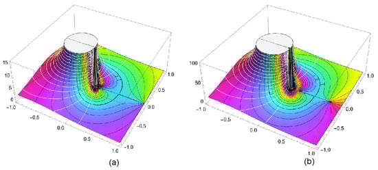  Figure 2. The 3D-complex plot of ${}_{\mu }\mathbf{A}_{\xi }^{\mu ,\nu }\left(\xi \right),{}_{\mu /2}\mathbf{A}_{\xi }^{\mu ,\nu }\left(\xi \right),\sigma \left(\xi \right)=\xi =x+iy$ accordingly, where the z-axis presents the operator ${}_{\mu }\mathbf{A}_{\xi }^{\mu ,\nu }\left(\xi \right)$ in (a) and ${}_{\mu /2}\mathbf{A}_{\xi }^{\mu ,\nu }\left(\xi \right)$ in (b).
• Three complex analytic functions are used to formulate the operator ${}_{\mathit{\ell }\hspace{1em}}{}^{\mathit{RL}}\mathcal{V}_{\xi }^{\mu ,\nu }\sigma \left(\xi \right)$: the fundamental function σ, the extreme function of starlikeness, and the normalized Fox-Wright function. But, the operator ${}_{\mathit{\ell }}{}^{\mathit{C}}\mathcal{V}_{\xi }^{\mu ,\nu }\sigma \left(\xi \right)$ is structured by double analytic functions. In the same way, for the integral operator ${}_{\mathit{\ell }}\mathit{A}_{\xi }^{\mu ,\nu }\sigma \left(\xi \right).$ As a conclusion of this point, the normalized $\mathit{\ell }-$fractal–fractional operators can be checked geometrically based on the properties of ${}_2\Psi _1^{\ast }$ (see Theorem 2).

The next step is to identify the geometrical characteristics that are crucial for the normalized ℓ-fractal–fractional operators.

4. Main Results

The fractal–fractional operators are employed in many scientific and technical disciplines and display a wide range of geometrical features. Fractal–fractional operators have unique geometric properties as they are memory-based and non-local. They are used in many fields, such as mathematics, physics, engineering, and image processing, to manage and understand complicated systems and patterns having fractal and self-similar qualities.

Theorem 2.

Suppose the normalized analytic function σ. If one of the following set of conditions (a) or (b) is achieved

(a)

$\mathit{\ell }>0,\mu <\mathit{\ell },\nu <2\mathit{\ell },n\ge 1;$ or

(b)

$\mathit{\ell }>0,\mu \ge \mathit{\ell },\nu <3\mathit{\ell }-\mu ,n\ge 1;$

together with the inequality

$$\begin{array}{c}\hfill |{\sigma }_n|<{\displaystyle \frac{\Gamma \left(2-\frac{\nu }{\mathit{\ell }}\right)\Gamma \left(n-\frac{-2\mathit{\ell }+\mu +\nu }{\mathit{\ell }}\right)}{n^2\Gamma \left(1-\frac{-2\mathit{\ell }+\mu +\nu }{\mathit{\ell }}\right)\Gamma \left(n-\frac{\nu }{\mathit{\ell }}+1\right)}}\end{array}$$

then ${}_{\mathit{\ell }}{}^{\mathit{C}}\mathcal{V}_{\xi }^{\mu ,\nu }\sigma \left(\xi \right)$ has a convex conduct.

If (a) or (b) is held together with the coefficients inequality

$$\begin{array}{c}\hfill |{\sigma }_n|<{\displaystyle \frac{2\Gamma \left(2-\frac{\nu }{\mathit{\ell }}\right)\Gamma \left(n-\frac{-2\mathit{\ell }+\mu +\nu }{\mathit{\ell }}\right)}{\sqrt{5}{n}^2\Gamma \left(1-\frac{-2\mathit{\ell }+\mu +\nu }{\mathit{\ell }}\right)\Gamma \left(n-\frac{\nu }{\mathit{\ell }}+1\right)}}\end{array}$$

then ${}_{\mathit{\ell }}{}^{\mathit{C}}\mathcal{V}_{\xi }^{\mu ,\nu }\sigma \left(\xi \right)$ has a starlike conduct.

Proof. 

In the sequel, we employ the following facts [13,14]

$$\begin{array}{cc}\hfill & \left|{\sigma }^{\prime }\left(\xi \right)-1\right|<1\Rightarrow \sigma isconvexin\left|\xi \right|<{\displaystyle \frac{1}{2}}\hfill \end{array}$$

(2)

$$\begin{array}{cc}\hfill & \left|{\sigma }^{\prime }\left(\xi \right)-1\right|<{\displaystyle \frac{2}{\sqrt{5}}}\Rightarrow \sigma isstarlikein\left|\xi \right|<{\displaystyle \frac{1}{2}}.\hfill \end{array}$$

(3)

Theorem 1 implies that ${}_{\mathit{\ell }}{}^{\mathbf{C}}\mathcal{V}_{\xi }^{\mu ,\nu }\sigma \left(\xi \right)$ is normalized and admitting the power series in (1). Furthermore, two normalized analytic functions of the kind (1) are obtained via certain features of the convolution product [15], and they fulfill

$$\begin{array}{c}\hfill {\left(\sigma \left(\xi \right)\ast \varsigma \left(\xi \right)\right)}^{\prime }={\displaystyle \frac{\sigma }{\xi }}\ast {\varsigma }^{\prime }\left(\xi \right).\xi \in \mathbb{O}.\end{array}$$

(4)

As a consequence, we obtain

$$\begin{array}{cc}\hfill {\left({}_{\mathit{\ell }}{}^{\mathbf{C}}\mathcal{V}_{\xi }^{\mu ,\nu }\sigma \left(\xi \right)\right)}^{\prime }& =\left({\displaystyle \frac{\xi {\sigma }^{\prime }\left(\xi \right)}{\xi }}\right)\ast {\left({}_2\Psi _1^{\ast }\left[\begin{array}{cc}(1,1)& (1-{\displaystyle \frac{\nu }{\mathit{\ell }}},1)\\ \left(-{\displaystyle \frac{-2\mathit{\ell }+\mu +\nu }{\mathit{\ell }}},1\right)\end{array};\xi \right]\right)}^{\prime }\hfill \\ \hfill & ={\sigma }^{\prime }\left(\xi \right)\ast {\left({}_2\Psi _1^{\ast }\left[\begin{array}{cc}(1,1)& (1-{\displaystyle \frac{\nu }{\mathit{\ell }}},1)\\ \left(-{\displaystyle \frac{-2\mathit{\ell }+\mu +\nu }{\mathit{\ell }}},1\right)\end{array};\xi \right]\right)}^{\prime }\hfill \\ \hfill & =\left(\sum _{n=1}^{\infty }n{\sigma }_n{\xi }^{n-1}\right)\ast \left(\left({\displaystyle \frac{\Gamma \left(1-\frac{-2\mathit{\ell }+\mu +\nu }{\mathit{\ell }}\right)}{\Gamma \left(2-\frac{\nu }{\mathit{\ell }}\right)}}\right)\sum _{n=1}^{\infty }\left({\displaystyle \frac{n\Gamma \left(n-\frac{\nu }{\mathit{\ell }}+1\right)}{\Gamma \left(n-\frac{-2\mathit{\ell }+\mu +\nu }{\mathit{\ell }}\right)}}\right){\xi }^{n-1}\right)\hfill \\ \hfill & =\left({\displaystyle \frac{\Gamma \left(1-\frac{-2\mathit{\ell }+\mu +\nu }{\mathit{\ell }}\right)}{\Gamma \left(2-\frac{\nu }{\mathit{\ell }}\right)}}\right)\sum _{n=1}^{\infty }\left({\displaystyle \frac{n^2{\sigma }_n\Gamma \left(n-\frac{\nu }{\mathit{\ell }}+1\right)}{\Gamma \left(n-\frac{-2\mathit{\ell }+\mu +\nu }{\mathit{\ell }}\right)}}\right){\xi }^{n-1},\hfill \end{array}$$

where ${\sigma }_1=1.$ Taking $\left|\xi \right|<1/2$ right here, and choosing option (a) or option (b), we obtain

$$\begin{array}{cc}\hfill \left|{\left({}_{\mathit{\ell }}{}^{\mathbf{C}}\mathcal{V}_{\xi }^{\mu ,\nu }\sigma \left(\xi \right)\right)}^{\prime }-1\right|& =\left|\left({\displaystyle \frac{\Gamma \left(1-\frac{-2\mathit{\ell }+\mu +\nu }{\mathit{\ell }}\right)}{\Gamma \left(2-\frac{\nu }{\mathit{\ell }}\right)}}\right)\sum _{n=2}^{\infty }\left({\displaystyle \frac{n^2{\sigma }_n\Gamma \left(n-\frac{\nu }{\mathit{\ell }}+1\right)}{\Gamma \left(n-\frac{-2\mathit{\ell }+\mu +\nu }{p}\right)}}\right){\xi }^{n-1}\right|\hfill \\ \hfill & \le \left({\displaystyle \frac{\Gamma \left(1-\frac{-2\mathit{\ell }+\mu +\nu }{\mathit{\ell }}\right)}{\Gamma \left(2-\frac{\nu }{\mathit{\ell }}\right)}}\right)\sum _{n=2}^{\infty }\left({\displaystyle \frac{n^2\left|{\sigma }_n\right|\Gamma \left(n-\frac{\nu }{\mathit{\ell }}+1\right)}{\Gamma \left(n-\frac{-2\mathit{\ell }+\mu +\nu }{\mathit{\ell }}\right)}}\right)\left|{\xi }^{n-1}\right|\hfill \\ \hfill & \le \left({\displaystyle \frac{\Gamma \left(1-\frac{-2\mathit{\ell }+\mu +\nu }{\mathit{\ell }}\right)}{\Gamma \left(2-\frac{\nu }{\mathit{\ell }}\right)}}\right)\sum _{n=2}^{\infty }\left({\displaystyle \frac{n^2\left|{\sigma }_n\right|\Gamma \left(n-\frac{\nu }{\mathit{\ell }}+1\right)}{\Gamma \left(n-\frac{-2\mathit{\ell }+\mu +\nu }{\mathit{\ell }}\right)}}\right){\displaystyle \frac{1}{2^{n-1}}}.\hfill \end{array}$$

Considering the prerequisite of the coefficient, the result is

$$\left({\displaystyle \frac{\Gamma \left(1-\frac{-2\mathit{\ell }+\mu +\nu }{\mathit{\ell }}\right)}{\Gamma \left(2-\frac{\nu }{\mathit{\ell }}\right)}}\right)\left({\displaystyle \frac{n^2\left|{\sigma }_n\right|\Gamma \left(n-\frac{\nu }{\mathit{\ell }}+1\right)}{\Gamma \left(n-\frac{-2\mathit{\ell }+\mu +\nu }{\mathit{\ell }}\right)}}\right)<1,$$

that is

$$\begin{array}{cc}\hfill \left|{\left({}_{\mathit{\ell }}{}^{\mathbf{C}}\mathcal{V}_{\xi }^{\mu ,\nu }\sigma \left(\xi \right)\right)}^{\prime }-1\right|& <\sum _{n=2}^{\infty }{\displaystyle \frac{1}{2^{n-1}}}=1.\hfill \end{array}$$

Consequently, we obtain

$$\left|{\left({}_{\mathit{\ell }}{}^{\mathbf{C}}\mathcal{V}_{\xi }^{\mu ,\nu }\sigma \left(\xi \right)\right)}^{\prime }-1\right|<1,$$

which means that the operator ${}_{\mathit{\ell }}{}^{\mathbf{C}}\mathcal{V}_{\xi }^{\mu ,\nu }\sigma \left(\xi \right)$ is convex (see inequality (2) for $\left|\xi \right|<1/2$). Likely, utilizing the coefficient condition,

$$\left({\displaystyle \frac{\Gamma \left(1-\frac{-2\mathit{\ell }+\mu +\nu }{\mathit{\ell }}\right)}{\Gamma \left(2-\frac{\nu }{\mathit{\ell }}\right)}}\right)\left({\displaystyle \frac{n^2\left|{\sigma }_n\right|\Gamma \left(n-\frac{\nu }{\mathit{\ell }}+1\right)}{\Gamma \left(n-\frac{-2\mathit{\ell }+\mu +\nu }{\mathit{\ell }}\right)}}\right)<{\displaystyle \frac{2}{\sqrt{5}}},$$

we have

$$\left|{\left({}_{\mathit{\ell }}{}^{\mathbf{C}}\mathcal{V}_{\xi }^{\mu ,\nu }\sigma \left(\xi \right)\right)}^{\prime }-1\right|<{\displaystyle \frac{2}{\sqrt{5}}},$$

which means that the operator ${}_{\mathit{\ell }}{}^{\mathbf{C}}\mathcal{V}_{\xi }^{\mu ,\nu }\sigma \left(\xi \right)$ is starlike (see inequality (3) for $\left|\xi \right|<1/2$). □

Theorem 3.

Consider the normalized analytic function σ. If $\mathit{\ell }>0,\mu <\mathit{\ell }$ and for $n\ge 1$ the inequality

$$\begin{array}{c}\hfill |{\sigma }_n|<{\displaystyle \frac{(2\mathit{\ell }-\mu )\Gamma (n-\mu /\mathit{\ell }+2)}{n\Gamma (n+1)\Gamma (3-\mu /\mathit{\ell })\left((n+1)\mathit{\ell }-\mu \right)}},n\ge 1\end{array}$$

is achieved, then ${}_{\mathit{\ell }\hspace{1em}}{}^{\mathit{RL}}\mathcal{V}_{\xi }^{\mu ,\nu }\sigma \left(\xi \right)$ admits a convex conduct. Moreover, if $\mathit{\ell }>0,\mu <\mathit{\ell }$ with the coefficients inequality

$$\begin{array}{c}\hfill |{\sigma }_n|<{\displaystyle \frac{2(2\mathit{\ell }-\mu )\Gamma (n-\mu /\mathit{\ell }+2)}{\sqrt{5}n\Gamma (n+1)\Gamma (3-\mu /\mathit{\ell })\left((n+1)\mathit{\ell }-\mu \right)}},n\ge 1\end{array}$$

then ${}_{\mathit{\ell }\hspace{1em}}{}^{\mathit{RL}}\mathcal{V}_{\xi }^{\mu ,\nu }\sigma \left(\xi \right)$ is starlike (see inequality (3) for $\left|\xi \right|<1/2$).

Proof. 

By employing (4), we observe that

$$\begin{array}{cc}\hfill & {\left({}_{\mathit{\ell }\hspace{1em}}{}^{\mathbf{RL}}\mathcal{V}_{\xi }^{\mu ,\nu }\sigma \left(\xi \right)\right)}^{\prime }\hfill \\ \hfill & ={\displaystyle \frac{\sigma \left(\xi \right)}{\xi }}\ast {\displaystyle \frac{\left({\displaystyle \frac{\xi }{{(1-\xi )}^2}}\left({\displaystyle \frac{\mu +\mathit{\ell }\xi -2\mathit{\ell }-\mu \xi }{\mu -2\mathit{\ell }}}\right)\right)}{\xi }}\ast {\left({}_2\Psi _1^{\ast }\left[\begin{array}{cc}(1,1)& (1,1)\\ (-\mu /\mathit{\ell }+2,1)\end{array};\xi \right]\right)}^{\prime }\hfill \\ \hfill & =\left(\sum _{n=1}^{\infty }{\sigma }_n{\xi }^{n-1}\right)\ast \left(\sum _{n=1}^{\infty }{\displaystyle \frac{(-\mu +(n+1)\mathit{\ell })}{(-\mu +2\mathit{\ell })}}{\xi }^{n-1}\right)\ast \left(\Gamma (3-\mu /\mathit{\ell })\sum _{n=1}^{\infty }n\left({\displaystyle \frac{\Gamma (n+1)}{\Gamma (n-\mu /\mathit{\ell }+2)}}\right){\xi }^{n-1}\right)\hfill \\ \hfill & =\left(\Gamma (3-\mu /\mathit{\ell })\sum _{n=1}^{\infty }n{\sigma }_n\left({\displaystyle \frac{(-\mu +(n+1)\mathit{\ell })}{(-\mu +2\mathit{\ell })}}\right)\left({\displaystyle \frac{\Gamma (n+1)}{\Gamma (n-\mu /\mathit{\ell }+2)}}\right){\xi }^{n-1}\right),{\sigma }_1=1.\hfill \end{array}$$

In view of the condition on the coefficients, we obtain

$$\begin{array}{cc}\hfill & \left|{\left({}_{\mathit{\ell }}{}^{\mathbf{RL}}\mathcal{V}_{\xi }^{\mu ,\nu }\sigma \left(\xi \right)\right)}^{\prime }-1\right|\hfill \\ \hfill & =\left|\left(\Gamma (3-\mu /\mathit{\ell })\sum _{n=2}^{\infty }n{\sigma }_n\left({\displaystyle \frac{(-\mu +(n+1)\mathit{\ell })}{(-\mu +2\mathit{\ell })}}\right)\left({\displaystyle \frac{\Gamma (n+1)}{\Gamma (n-\mu /\mathit{\ell }+2)}}\right){\xi }^{n-1}\right)\right|\hfill \\ \hfill & \le \left(\Gamma (3-\mu /\mathit{\ell })\sum _{n=2}^{\infty }n\left|{\sigma }_n\right|\left({\displaystyle \frac{(n+1)\mathit{\ell }-\mu }{2\mathit{\ell }-\mu }}\right)\left({\displaystyle \frac{\Gamma (n+1)}{\Gamma (n-\mu /\mathit{\ell }+2)}}\right)\left|{\xi }^{n-1}\right|\right)\hfill \\ \hfill & <\left(\Gamma (3-\mu /\mathit{\ell })\sum _{n=2}^{\infty }n\left|{\sigma }_n\right|\left({\displaystyle \frac{(n+1)\mathit{\ell }-\mu }{2\mathit{\ell }-\mu }}\right)\left({\displaystyle \frac{\Gamma (n+1)}{\Gamma (n-\mu /\mathit{\ell }+2)}}\right)\left({\displaystyle \frac{1}{2^{n-1}}}\right)\right).\hfill \end{array}$$

As

$$\left|{\sigma }_n\right|<{\displaystyle \frac{(2\mathit{\ell }-\mu )\Gamma (n-\mu /\mathit{\ell }+2)}{n\Gamma (n+1)\Gamma (3-\mu /\mathit{\ell })\left((n+1)\mathit{\ell }-\mu \right)}}$$

then

$$\begin{array}{cc}\hfill \left|{\left({}_{\mathit{\ell }\hspace{1em}}{}^{\mathbf{RL}}\mathcal{V}_{\xi }^{\mu ,\nu }\sigma \left(\xi \right)\right)}^{\prime }-1\right|& <\sum _{n=2}^{\infty }\left({\displaystyle \frac{1}{2^{n-1}}}\right)=1.\hfill \end{array}$$

Therefore, by (2), we obtain that $\left({}_{\mathit{\ell }\hspace{1em}}{}^{\mathbf{RL}}\mathcal{V}_{\xi }^{\mu ,\nu }\sigma \left(\xi \right)\right)$ is convex in $\left|\xi \right|<1/2$. In addition, the inequality

$$\begin{array}{c}\hfill |{\sigma }_n|<{\displaystyle \frac{2(2\mathit{\ell }-\mu )\Gamma (n-\mu /\mathit{\ell }+2)}{\sqrt{5}n\Gamma (n+1)\Gamma (3-\mu /\mathit{\ell })\left((n+1)\mathit{\ell }-\mu \right)}}\end{array}$$

yields

$$\begin{array}{cc}\hfill \left|{\left({}_{\mathit{\ell }\hspace{1em}}{}^{\mathbf{RL}}\mathcal{V}_{\xi }^{\mu ,\nu }\sigma \left(\xi \right)\right)}^{\prime }-1\right|& <{\displaystyle \frac{2}{\sqrt{5}}}\sum _{n=2}^{\infty }\left({\displaystyle \frac{1}{2^{n-1}}}\right)={\displaystyle \frac{2}{\sqrt{5}}}.\hfill \end{array}$$

Hence, (3), implies $\left({}_{\mathit{\ell }\hspace{1em}}{}^{\mathbf{RL}}\mathcal{V}_{\xi }^{\mu ,\nu }\sigma \left(\xi \right)\right)$ is starlike in $\left|\xi \right|<1/2$. □

Theorem 4.

For the normalized analytic function σ, if

$$\begin{array}{c}\hfill |{\sigma }_n|<{\displaystyle \frac{\Gamma \left(1+\frac{\mu }{\mathit{\ell }}\right)\Gamma \left(n+\frac{2\mu }{\mathit{\ell }}\right)}{n\Gamma \left(1+\frac{2\mu }{\mathit{\ell }}\right)\Gamma \left(n+\frac{\mu }{\mathit{\ell }}\right)}},n\ge 1,\mathit{\ell }>0,\mu >0\end{array}$$

then ${}_{\mathit{\ell }}\mathit{A}_{\xi }^{\mu ,\nu }\sigma \left(\xi \right)$ is convex. Moreover, if

$$\begin{array}{c}\hfill |{\sigma }_n|<{\displaystyle \frac{2\Gamma \left(1+\frac{\mu }{\mathit{\ell }}\right)\Gamma \left(n+\frac{2\mu }{\mathit{\ell }}\right)}{\sqrt{5}n\Gamma \left(1+\frac{2\mu }{\mathit{\ell }}\right)\Gamma \left(n+\frac{\mu }{\mathit{\ell }}\right)}},n\ge 1,\mathit{\ell }>0,\mu >0\end{array}$$

then ${}_{\mathit{\ell }}\mathit{A}_{\xi }^{\mu ,\nu }\sigma \left(\xi \right)$ is starlike.

Proof. 

From (4), we obtain

$$\begin{array}{cc}\hfill {\left({}_{\mathit{\ell }}\mathbf{A}_{\xi }^{\mu ,\nu }\sigma \left(\xi \right)\right)}^{\prime }& ={\displaystyle \frac{\sigma \left(\xi \right)}{\xi }}\ast {\left({}_2\Psi _1^{\ast }\left[\begin{array}{cc}(1,1)& (\mu /\mathit{\ell },1)\\ (2\mu /\mathit{\ell },1)\end{array};\xi \right]\right)}^{\prime }\hfill \\ \hfill & =\left(\sum _{n=1}^{\infty }{\sigma }_n{\xi }^{n-1}\right)\ast \left(\left({\displaystyle \frac{\Gamma \left(1+\frac{2\mu }{\mathit{\ell }}\right)}{\Gamma \left(1+\frac{\mu }{\mathit{\ell }}\right)}}\right)\sum _{n=1}^{\infty }n\left({\displaystyle \frac{\Gamma \left(n+\frac{\mu }{\mathit{\ell }}\right)}{\Gamma \left(n+\frac{2\mu }{\mathit{\ell }}\right)}}\right){\xi }^{n-1}\right)\hfill \\ \hfill & =\left(\left({\displaystyle \frac{\Gamma \left(1+\frac{2\mu }{\mathit{\ell }}\right)}{\Gamma \left(1+\frac{\mu }{\mathit{\ell }}\right)}}\right)\sum _{n=1}^{\infty }n{\sigma }_n\left({\displaystyle \frac{\Gamma \left(n+\frac{\mu }{\mathit{\ell }}\right)}{\Gamma \left(n+\frac{2\mu }{\mathit{\ell }}\right)}}\right){\xi }^{n-1}\right)\hfill \end{array}$$

By the condition on the coefficient, we obtain

$$\begin{array}{cc}\hfill & \left|{\left({}_{\mathit{\ell }}\mathbf{A}_{\xi }^{\mu ,\nu }\sigma \left(\xi \right)\right)}^{\prime }-1\right|\hfill \\ \hfill & =\left|\left(\left({\displaystyle \frac{\Gamma \left(1+\frac{2\mu }{\mathit{\ell }}\right)}{\Gamma \left(1+\frac{\mu }{\mathit{\ell }}\right)}}\right)\sum _{n=2}^{\infty }n{\sigma }_n\left({\displaystyle \frac{\Gamma \left(n+\frac{\mu }{\mathit{\ell }}\right)}{\Gamma \left(n+\frac{2\mu }{\mathit{\ell }}\right)}}\right){\xi }^{n-1}\right)\right|\hfill \\ \hfill & \le \left(\left({\displaystyle \frac{\Gamma \left(1+\frac{2\mu }{\mathit{\ell }}\right)}{\Gamma \left(1+\frac{\mu }{\mathit{\ell }}\right)}}\right)\sum _{n=1}^{\infty }n|{\sigma }_n|\left({\displaystyle \frac{\Gamma \left(n+\frac{\mu }{\mathit{\ell }}\right)}{\Gamma \left(n+\frac{2\mu }{\mathit{\ell }}\right)}}\right)\left|{\xi }^{n-1}\right|\right)\hfill \\ \hfill & <\left(\left({\displaystyle \frac{\Gamma \left(1+\frac{2\mu }{\mathit{\ell }}\right)}{\Gamma \left(1+\frac{\mu }{\mathit{\ell }}\right)}}\right)\sum _{n=1}^{\infty }n\left|{\sigma }_n\right|\left({\displaystyle \frac{\Gamma \left(n+\frac{\mu }{\mathit{\ell }}\right)}{\Gamma \left(n+\frac{2\mu }{\mathit{\ell }}\right)}}\right)\left({\displaystyle \frac{1}{2^{n-1}}}\right)\right).\hfill \end{array}$$

Since

$$\left|{\sigma }_n\right|<{\displaystyle \frac{\Gamma \left(1+\frac{\mu }{\mathit{\ell }}\right)\Gamma \left(n+\frac{2\mu }{\mathit{\ell }}\right)}{n\Gamma \left(1+\frac{2\mu }{\mathit{\ell }}\right)\Gamma \left(n+\frac{\mu }{\mathit{\ell }}\right)}}$$

then

$$\begin{array}{cc}\hfill \left|{\left({}_{\mathit{\ell }}\mathbf{A}_{\xi }^{\mu ,\nu }\sigma \left(\xi \right)\right)}^{\prime }-1\right|& <\sum _{n=2}^{\infty }\left({\displaystyle \frac{1}{2^{n-1}}}\right)=1.\hfill \end{array}$$

According to (2), we obtain $\left({}_{\mathit{\ell }}\mathbf{A}_{\xi }^{\mu ,\nu }\sigma \left(\xi \right)\right)$ is convex in $\left|\xi \right|<1/2$. Next, by

$$\begin{array}{c}\hfill |{\sigma }_n|<{\displaystyle \frac{2\Gamma \left(1+\frac{\mu }{\mathit{\ell }}\right)\Gamma \left(n+\frac{2\mu }{\mathit{\ell }}\right)}{\sqrt{5}n\Gamma \left(1+\frac{2\mu }{\mathit{\ell }}\right)\Gamma \left(n+\frac{\mu }{\mathit{\ell }}\right)}}\end{array}$$

implies

$$\begin{array}{cc}\hfill \left|{\left({}_{\mathit{\ell }}\mathbf{A}_{\xi }^{\mu ,\nu }\sigma \left(\xi \right)\right)}^{\prime }-1\right|& <{\displaystyle \frac{2}{\sqrt{5}}}\sum _{n=2}^{\infty }\left({\displaystyle \frac{1}{2^{n-1}}}\right)={\displaystyle \frac{2}{\sqrt{5}}}.\hfill \end{array}$$

Thus, (3) implies $\left({}_{\mathit{\ell }}\mathbf{A}_{\xi }^{\mu ,\nu }\sigma \left(\xi \right)\right)$ is starlike in $\left|\xi \right|<1/2$. □

We address the boundedness of the $\mathit{\ell }-$fractal–fractional operators in the unit disk in the subsequent phase of our study.

5. Boundedness of ℓ-Fractal–Fractional Operator

Boundedness is an important concept in complex analysis and complex function theory, as it may be applied to define the behavior of functions or sequences through certain regions of the complex plane. Bounded functions within the open unit disk often have advantageous mathematical properties and are easier to measure than unbounded functions. The boundedness of the $\mathit{\ell }-$fractal–fractional operators in the unit disk when a geometric characteristic is admitted by the normalized analytic function is then discussed.

Theorem 5.

Consider the normalized analytic function σ is a convex. Then, the $\mathit{\ell }-$fractal–fractional operators are bounded in the unit disk, with

• $$\left|\left({}_{\mathit{\ell }}{}^{\mathit{C}}\mathcal{V}_{\xi }^{\mu ,\nu }\sigma \left(\xi \right)\right)\right|\le r\left({}_2\Psi _1^{\ast }\left[\begin{array}{cc}(2,1)& (2-{\displaystyle \frac{\nu }{\mathit{\ell }}},1)\\ \left(1-{\displaystyle \frac{-2\mathit{\ell }+\mu +\nu }{\mathit{\ell }}},1\right)\end{array};r\right]\right);$$
• $$\left|\left({}_{\mathit{\ell }\hspace{1em}}{}^{\mathit{RL}}\mathcal{V}_{\xi }^{\mu ,\nu }\sigma \left(\xi \right)\right)\right|\le \left({\displaystyle \frac{(1-r)(\mathit{\ell }-\mu )(-log(1-r\left)\right)+\mathit{\ell }r}{(1-r)(2\mathit{\ell }-\mu )}}\right)\left({}_2\Psi _1^{\ast }\left[\begin{array}{cc}(2,1)& (2,1)\\ (-\mu /\mathit{\ell }+3,1)\end{array};r\right]\right);$$
• $$\left|\left({}_{\mathit{\ell }}\mathit{A}_{\xi }^{\mu ,\nu }\sigma \left(\xi \right)\right)\right|\le r\left({}_2\Psi _1^{\ast }\left[\begin{array}{cc}(1,1)& (1+\mu /\mathit{\ell },1)\\ (1+2\mu /\mathit{\ell },1)\end{array};r\right]\right),$$

where $\mathit{\ell }>\mu ,\left|\xi \right|=r<1.$

Proof. 

Let $\sigma \left(\xi \right)$ in (1) be convex. As a consequence, we obtain $|{\sigma }_n|\le 1$. Theorem 1 implies that

$$\begin{array}{cc}\hfill \left|{}_{\mathit{\ell }}{}^{\mathbf{C}}\mathcal{V}_{\xi }^{\mu ,\nu }\sigma \left(\xi \right)\right|& \le \left({\displaystyle \frac{\Gamma \left(1-\frac{-2\mathit{\ell }+\mu +\nu }{\mathit{\ell }}\right)}{\Gamma \left(1-\frac{\nu }{\mathit{\ell }}+1\right)}}\right)\sum _{n=1}^{\infty }n\left|{\sigma }_n\right|\left({\displaystyle \frac{\Gamma (n+1)\Gamma \left(n-\frac{\nu }{\mathit{\ell }}+1\right)}{\Gamma \left(n-\frac{-2\mathit{\ell }+\mu +\nu }{p}\right)}}\right){\displaystyle \frac{|{\xi }^n|}{n!}}\hfill \\ \hfill & \le \left({\displaystyle \frac{\Gamma \left(1-\frac{-2\mathit{\ell }+\mu +\nu }{\mathit{\ell }}\right)}{\Gamma \left(1-\frac{\nu }{\mathit{\ell }}+1\right)}}\right)\sum _{n=1}^{\infty }n\left({\displaystyle \frac{\Gamma (n+1)\Gamma \left(n-\frac{\nu }{\mathit{\ell }}+1\right)}{\Gamma \left(n-\frac{-2\mathit{\ell }+\mu +\nu }{\mathit{\ell }}\right)}}\right){\displaystyle \frac{r^n}{n!}}\hfill \\ \hfill & =r\left({\displaystyle \frac{\Gamma \left(1-\frac{-2\mathit{\ell }+\mu +\nu }{\mathit{\ell }}\right)}{\Gamma \left(1-\frac{\nu }{\mathit{\ell }}+1\right)}}\right)\sum _{n=0}^{\infty }\left({\displaystyle \frac{\Gamma (n+2)\Gamma \left(n+1-\frac{\nu }{\mathit{\ell }}+1\right)}{\Gamma \left(n+1-\frac{-2\mathit{\ell }+\mu +\nu }{\mathit{\ell }}\right)}}\right){\displaystyle \frac{r^n}{n!}}\hfill \\ \hfill & =r\left({}_2\Psi _1^{\ast }\left[\begin{array}{cc}(2,1)& (2-{\displaystyle \frac{\nu }{\mathit{\ell }}},1)\\ \left(1-{\displaystyle \frac{-2\mathit{\ell }+\mu +\nu }{\mathit{\ell }}},1\right)\end{array};r\right]\right).\hfill \end{array}$$

For ${}_{\mathit{\ell }\hspace{1em}}{}^{\mathbf{RL}}\mathcal{V}_{\xi }^{\mu ,\nu }\sigma \left(\xi \right),$ and by the Young’s inequality of convolution product, we have

$$\begin{array}{cc}\hfill \left|{}_{\mathit{\ell }\hspace{1em}}{}^{\mathbf{RL}}\mathcal{V}_{\xi }^{\mu ,\nu }\sigma \left(\xi \right)\right|& \le \Gamma (3-\mu /\mathit{\ell })\sum _{n=1}^{\infty }\left|{\sigma }_n\right|\left({\displaystyle \frac{\Gamma (n+1)\Gamma (n+1)}{\Gamma (n-\mu /\mathit{\ell }+2)}}\right)\left|{\displaystyle \frac{(-\mu +(n+1)\mathit{\ell })}{(-\mu +2\mathit{\ell })}}\right|{\displaystyle \frac{{\left|\xi \right|}^n}{n!}}\hfill \\ \hfill & \le \Gamma (3-\mu /\mathit{\ell })\sum _{n=1}^{\infty }\left({\displaystyle \frac{\Gamma (n+1)\Gamma (n+1)}{\Gamma (n-\mu /\mathit{\ell }+2)}}\right)\left|{\displaystyle \frac{(-\mu +(n+1)\mathit{\ell })}{(-\mu +2\mathit{\ell })}}\right|{\displaystyle \frac{r^n}{n!}}\hfill \\ \hfill & =r\Gamma (3-\mu /\mathit{\ell })\sum _{n=0}^{\infty }\left({\displaystyle \frac{\Gamma (n+2)\Gamma (n+2)}{\Gamma (n-\mu /\mathit{\ell }+3)}}\right)\left|{\displaystyle \frac{(-\mu +(n+2)\mathit{\ell })}{(-\mu +2\mathit{\ell })(n+1)}}\right|{\displaystyle \frac{r^n}{n!}}\hfill \\ \hfill & \le \left({\displaystyle \frac{\left(\right(1-r\left)\right(\mathit{\ell }-\mu )log(1-r)+\mathit{\ell }r)}{\left(\right(r-1\left)r\right(2\mathit{\ell }-\mu \left)\right)}}\right)r\left({}_2\Psi _1^{\ast }\left[\begin{array}{cc}(2,1)& (2,1)\\ (-\mu /\mathit{\ell }+3,1)\end{array};r\right]\right)\hfill \\ \hfill & =\left({\displaystyle \frac{(1-r)(\mathit{\ell }-\mu )(-log(1-r\left)\right)+\mathit{\ell }r}{(1-r)(2\mathit{\ell }-\mu )}}\right)\left({}_2\Psi _1^{\ast }\left[\begin{array}{cc}(2,1)& (2,1)\\ (-\mu /\mathit{\ell }+3,1)\end{array};r\right]\right),\mathit{\ell }>\mu .\hfill \end{array}$$

Obtaining the integral operator

$$\begin{array}{cc}\hfill \left|{}_{\mathit{\ell }}\mathbf{A}_{\xi }^{\mu ,\nu }\sigma \left(\xi \right)\right|& \le \left({\displaystyle \frac{\Gamma \left(1+\frac{2\mu }{\mathit{\ell }}\right)}{\Gamma \left(1+\frac{\mu }{\mathit{\ell }}\right)}}\right)\sum _{n=1}^{\infty }\left|{\sigma }_n\right|\left({\displaystyle \frac{\Gamma (n+1)\Gamma \left(n+\frac{\mu }{\mathit{\ell }}\right)}{\Gamma \left(n+\frac{2\mu }{\mathit{\ell }}\right)}}\right){\displaystyle \frac{{\left|\xi \right|}^n}{n!}}\hfill \\ \hfill & \le \left({\displaystyle \frac{\Gamma \left(1+\frac{2\mu }{\mathit{\ell }}\right)}{\Gamma \left(1+\frac{\mu }{\mathit{\ell }}\right)}}\right)\sum _{n=1}^{\infty }\left({\displaystyle \frac{\Gamma (n+1)\Gamma \left(n+\frac{\mu }{\mathit{\ell }}\right)}{\Gamma \left(n+\frac{2\mu }{\mathit{\ell }}\right)}}\right){\displaystyle \frac{r^n}{n!}}\hfill \\ \hfill & =r\left({\displaystyle \frac{\Gamma \left(1+\frac{2\mu }{\mathit{\ell }}\right)}{\Gamma \left(1+\frac{\mu }{\mathit{\ell }}\right)}}\right)\sum _{n=0}^{\infty }\left({\displaystyle \frac{\Gamma (n+2)\Gamma \left(n+1+\frac{\mu }{\mathit{\ell }}\right)}{\Gamma \left(n+1+\frac{2\mu }{\mathit{\ell }}\right)}}\right){\displaystyle \frac{r^n}{(n+1)n!}}\hfill \\ \hfill & =r\left({\displaystyle \frac{\Gamma \left(1+\frac{2\mu }{\mathit{\ell }}\right)}{\Gamma \left(1+\frac{\mu }{\mathit{\ell }}\right)}}\right)\sum _{n=0}^{\infty }\left({\displaystyle \frac{\Gamma (n+1)\Gamma \left(n+1+\frac{\mu }{\mathit{\ell }}\right)}{\Gamma \left(n+1+\frac{2\mu }{\mathit{\ell }}\right)}}\right){\displaystyle \frac{r^n}{n!}}\hfill \\ \hfill & =r\left({}_2\Psi _1^{\ast }\left[\begin{array}{cc}(1,1)& (1+\mu /\mathit{\ell },1)\\ (1+2\mu /\mathit{\ell },1)\end{array};r\right]\right).\hfill \end{array}$$

□

Example 4.

Assume that $\sigma \left(\xi \right)={\displaystyle \frac{\xi }{1-\xi }},$ which is the extreme convex function in the open unit disk. Then, in view of Theorem 5, we have

• $$\left|\left({}_{\mathit{\ell }}{}^{\mathit{C}}\mathcal{V}_{\xi }^{\mu ,\nu }\left({\displaystyle \frac{\xi }{1-\xi }}\right)\right)\right|\le r\left({}_2\Psi _1^{\ast }\left[\begin{array}{cc}(2,1)& (2-{\displaystyle \frac{\nu }{\mathit{\ell }}},1)\\ \left(1-{\displaystyle \frac{-2\mathit{\ell }+\mu +\nu }{\mathit{\ell }}},1\right)\end{array};r\right]\right);$$
• $$\left|\left({}_{\mathit{\ell }\hspace{1em}}{}^{\mathit{RL}}\mathcal{V}_{\xi }^{\mu ,\nu }\left({\displaystyle \frac{\xi }{1-\xi }}\right)\right)\right|\le \left({\displaystyle \frac{(1-r)(\mathit{\ell }-\mu )(-log(1-r\left)\right)+\mathit{\ell }r}{(1-r)(2\mathit{\ell }-\mu )}}\right)\left({}_2\Psi _1^{\ast }\left[\begin{array}{cc}(2,1)& (2,1)\\ (-\mu /\mathit{\ell }+3,1)\end{array};r\right]\right);$$
• $$\left|\left({}_{\mathit{\ell }}\mathit{A}_{\xi }^{\mu ,\nu }\left({\displaystyle \frac{\xi }{1-\xi }}\right)\right)\right|\le r\left({}_2\Psi _1^{\ast }\left[\begin{array}{cc}(1,1)& (1+\mu /\mathit{\ell },1)\\ (1+2\mu /\mathit{\ell },1)\end{array};r\right]\right),$$

where $\mathit{\ell }>\mu ,\left|\xi \right|=r<1.$

Theorem 6.

Assume that σ is starlike. Then, the $\mathit{\ell }-$fractal–fractional operators are bounded in the unit disk, with

• $$\left|\left({}_{\mathit{\ell }}{}^{\mathit{C}}\mathcal{V}_{\xi }^{\mu ,\nu }\sigma \left(\xi \right)\right)\right|\le {\displaystyle \frac{r}{{(1-r)}^2}}\left({}_2\Psi _1^{\ast }\left[\begin{array}{cc}(2,1)& (2-{\displaystyle \frac{\nu }{\mathit{\ell }}},1)\\ \left(1-{\displaystyle \frac{-2\mathit{\ell }+\mu +\nu }{\mathit{\ell }}},1\right)\end{array};r\right]\right);$$
• $$\left|\left({}_{\mathit{\ell }\hspace{1em}}{}^{\mathit{RL}}\mathcal{V}_{\xi }^{\mu ,\nu }\sigma \left(\xi \right)\right)\right|\le \left({\displaystyle \frac{r\left(\frac{\mathit{\ell }}{2\mathit{\ell }-\mu }-1\right)+1}{{(1-r)}^2}}\right)r\left({}_2\Psi _1^{\ast }\left[\begin{array}{cc}(2,1)& (2,1)\\ (-\mu /\mathit{\ell }+3,1)\end{array};r\right]\right),\mathit{\ell }>\mu /2;$$
• $$\left|\left({}_{\mathit{\ell }}\mathit{A}_{\xi }^{\mu ,\nu }\sigma \left(\xi \right)\right)\right|\le r\left({}_2\Psi _1^{\ast }\left[\begin{array}{cc}(2,1)& (1+\mu /\mathit{\ell },1)\\ (1+2\mu /\mathit{\ell },1)\end{array};r\right]\right),$$

where $\left|\xi \right|=r<1.$

Proof. 

As $\sigma$ is starlike, then $|{\sigma }_n|\le n.$ A computation implies that

$$\begin{array}{cc}\hfill \left|{}_{\mathit{\ell }}{}^{\mathbf{C}}\mathcal{V}_{\xi }^{\mu ,\nu }\sigma \left(\xi \right)\right|& \le \left({\displaystyle \frac{\Gamma \left(1-\frac{-2\mathit{\ell }+\mu +\nu }{\mathit{\ell }}\right)}{\Gamma \left(1-\frac{\nu }{\mathit{\ell }}+1\right)}}\right)\sum _{n=1}^{\infty }n\left|{\sigma }_n\right|\left({\displaystyle \frac{\Gamma (n+1)\Gamma \left(n-\frac{\nu }{\mathit{\ell }}+1\right)}{\Gamma \left(n-\frac{-2\mathit{\ell }+\mu +\nu }{\mathit{\ell }}\right)}}\right){\displaystyle \frac{|{\xi }^n|}{n!}}\hfill \\ \hfill & \le \left({\displaystyle \frac{\Gamma \left(1-\frac{-2\mathit{\ell }+\mu +\nu }{\mathit{\ell }}\right)}{\Gamma \left(1-\frac{\nu }{\mathit{\ell }}+1\right)}}\right)\sum _{n=1}^{\infty }{n}^2\left({\displaystyle \frac{\Gamma (n+1)\Gamma \left(n-\frac{\nu }{\mathit{\ell }}+1\right)}{\Gamma \left(n-\frac{-2\mathit{\ell }+\mu +\nu }{\mathit{\ell }}\right)}}\right){\displaystyle \frac{r^n}{n!}}\hfill \\ \hfill & =\left({\displaystyle \frac{\Gamma \left(1-\frac{-2\mathit{\ell }+\mu +\nu }{\mathit{\ell }}\right)}{\Gamma \left(1-\frac{\nu }{\mathit{\ell }}+1\right)}}\right)\sum _{n=1}^{\infty }n\left({\displaystyle \frac{\Gamma (n+1)\Gamma \left(n-\frac{\nu }{\mathit{\ell }}+1\right)}{\Gamma \left(n-\frac{-2\mathit{\ell }+\mu +\nu }{\mathit{\ell }}\right)}}\right){\displaystyle \frac{r^n}{(n-1)!}}\hfill \\ \hfill & =r\left({\displaystyle \frac{\Gamma \left(1-\frac{-2\mathit{\ell }+\mu +\nu }{\mathit{\ell }}\right)}{\Gamma \left(1-\frac{\nu }{\mathit{\ell }}+1\right)}}\right)\sum _{n=0}^{\infty }(n+1)\left({\displaystyle \frac{\Gamma (n+2)\Gamma \left(n+1-\frac{\nu }{\mathit{\ell }}+1\right)}{\Gamma \left(n+1-\frac{-2\mathit{\ell }+\mu +\nu }{\mathit{\ell }}\right)}}\right){\displaystyle \frac{r^n}{n!}}\hfill \\ \hfill & \le {\displaystyle \frac{r}{{(1-r)}^2}}\left({}_2\Psi _1^{\ast }\left[\begin{array}{cc}(2,1)& (2-{\displaystyle \frac{\nu }{\mathit{\ell }}},1)\\ \left(1-{\displaystyle \frac{-2\mathit{\ell }+\mu +\nu }{\mathit{\ell }}},1\right)\end{array};r\right]\right).\hfill \end{array}$$

Second inequality yields

$$\begin{array}{cc}\hfill \left|{}_{\mathit{\ell }\hspace{1em}}{}^{\mathbf{RL}}\mathcal{V}_{\xi }^{\mu ,\nu }\sigma \left(\xi \right)\right|& \le \Gamma (3-\mu /\mathit{\ell })\sum _{n=1}^{\infty }\left|{\sigma }_n\right|\left({\displaystyle \frac{\Gamma (n+1)\Gamma (n+1)}{\Gamma (n-\mu /\mathit{\ell }+2)}}\right)\left|{\displaystyle \frac{(-\mu +(n+1)\mathit{\ell })}{(-\mu +2\mathit{\ell })}}\right|{\displaystyle \frac{{\left|\xi \right|}^n}{n!}}\hfill \\ \hfill & \le \Gamma (3-\mu /\mathit{\ell })\sum _{n=1}^{\infty }\left({\displaystyle \frac{\Gamma (n+1)\Gamma (n+1)}{\Gamma (n-\mu /\mathit{\ell }+2)}}\right)\left|{\displaystyle \frac{(-\mu +(n+1)\mathit{\ell })}{(-\mu +2\mathit{\ell })}}\right|{\displaystyle \frac{r^n}{(n-1)!}}\hfill \\ \hfill & =r\Gamma (3-\mu /\mathit{\ell })\sum _{n=0}^{\infty }\left({\displaystyle \frac{\Gamma (n+2)\Gamma (n+2)}{\Gamma (n-\mu /\mathit{\ell }+3)}}\right)\left|{\displaystyle \frac{(-\mu +(n+2)\mathit{\ell })}{(-\mu +2\mathit{\ell })}}\right|{\displaystyle \frac{r^n}{n!}}\hfill \\ \hfill & \le \left({\displaystyle \frac{r\left(\frac{\mathit{\ell }}{2\mathit{\ell }-\mu }-1\right)+1}{{(1-r)}^2}}\right)r\left({}_2\Psi _1^{\ast }\left[\begin{array}{cc}(2,1)& (2,1)\\ (-\mu /\mathit{\ell }+3,1)\end{array};r\right]\right),\mathit{\ell }>\mu /2.\hfill \end{array}$$

Lastly, we find for the integral operator

$$\begin{array}{cc}\hfill \left|{}_{\mathit{\ell }}\mathbf{A}_{\xi }^{\mu ,\nu }\sigma \left(\xi \right)\right|& \le \left({\displaystyle \frac{\Gamma \left(1+\frac{2\mu }{\mathit{\ell }}\right)}{\Gamma \left(1+\frac{\mu }{\mathit{\ell }}\right)}}\right)\sum _{n=1}^{\infty }\left|{\sigma }_n\right|\left({\displaystyle \frac{\Gamma (n+1)\Gamma \left(n+\frac{\mu }{\mathit{\ell }}\right)}{\Gamma \left(n+\frac{2\mu }{\mathit{\ell }}\right)}}\right){\displaystyle \frac{{\left|\xi \right|}^n}{n!}}\hfill \\ \hfill & \le \left({\displaystyle \frac{\Gamma \left(1+\frac{2\mu }{\mathit{\ell }}\right)}{\Gamma \left(1+\frac{\mu }{\mathit{\ell }}\right)}}\right)\sum _{n=1}^{\infty }\left({\displaystyle \frac{\Gamma (n+1)\Gamma \left(n+\frac{\mu }{\mathit{\ell }}\right)}{\Gamma \left(n+\frac{2\mu }{\mathit{\ell }}\right)}}\right){\displaystyle \frac{r^n}{(n-1)!}}\hfill \\ \hfill & =r\left({\displaystyle \frac{\Gamma \left(1+\frac{2\mu }{\mathit{\ell }}\right)}{\Gamma \left(1+\frac{\mu }{\mathit{\ell }}\right)}}\right)\sum _{n=0}^{\infty }\left({\displaystyle \frac{\Gamma (n+2)\Gamma \left(n+1+\frac{\mu }{\mathit{\ell }}\right)}{\Gamma \left(n+1+\frac{2\mu }{p}\right)}}\right){\displaystyle \frac{r^n}{n!}}\hfill \\ \hfill & \le r\left({}_2\Psi _1^{\ast }\left[\begin{array}{cc}(2,1)& (1+\mu /\mathit{\ell },1)\\ (1+2\mu /\mathit{\ell },1)\end{array};r\right]\right).\hfill \end{array}$$

□

Example 5.

Assume that $\sigma \left(\xi \right)={\displaystyle \frac{\xi }{{(1-\xi )}^2}},$ which is the extreme starlike function in the open unit disk. Then, in view of Theorem 6, we have

• $$\left|\left({}_{\mathit{\ell }}{}^{\mathit{C}}\mathcal{V}_{\xi }^{\mu ,\nu }\left({\displaystyle \frac{\xi }{{(1-\xi )}^2}}\right)\right)\right|\le {\displaystyle \frac{r}{{(1-r)}^2}}\left({}_2\Psi _1^{\ast }\left[\begin{array}{cc}(2,1)& (2-{\displaystyle \frac{\nu }{\mathit{\ell }}},1)\\ \left(1-{\displaystyle \frac{-2\mathit{\ell }+\mu +\nu }{\mathit{\ell }}},1\right)\end{array};r\right]\right);$$
• $$\left|\left({}_{\mathit{\ell }\hspace{1em}}{}^{\mathit{RL}}\mathcal{V}_{\xi }^{\mu ,\nu }\left({\displaystyle \frac{\xi }{{(1-\xi )}^2}}\right)\right)\right|\le \left({\displaystyle \frac{r\left(\frac{\mathit{\ell }}{2\mathit{\ell }-\mu }-1\right)+1}{{(1-r)}^2}}\right)r\left({}_2\Psi _1^{\ast }\left[\begin{array}{cc}(2,1)& (2,1)\\ (-\mu /\mathit{\ell }+3,1)\end{array};r\right]\right),\mathit{\ell }>\mu /2;$$
• $$\left|\left({}_{\mathit{\ell }}\mathit{A}_{\xi }^{\mu ,\nu }\left({\displaystyle \frac{\xi }{{(1-\xi )}^2}}\right)\right)\right|\le r\left({}_2\Psi _1^{\ast }\left[\begin{array}{cc}(2,1)& (1+\mu /\mathit{\ell },1)\\ (1+2\mu /\mathit{\ell },1)\end{array};r\right]\right),$$

6. Conclusions

We created a generalization of the most recent work on fractal–fractional operators utilizing the power products, based on the expanded gamma function or $\mathit{\ell }-$gamma function. We demonstrate the usefulness of these operations with certain cases. All kinds of fractional differential equations, dynamic systems, thermal inquires, specific transformations (derivatives and integrals, among them heat and wave transformations), and computational investigations are all capable of being generalized by the suggested $\mathit{\ell }-$fractal–fractional. Employing a complex variable, we created the $\mathit{\ell }-$fractal–fractional operators. Geometrical and analytical phenomena are investigated. It is proposed to use these operators on an open unit disk normalized analytic function. Additionally, the operators are regarded as belonging to the class of normalized functions under a certain formula involving these operators. Consequently, we provided the requirements for these operators to meet the two most crucial geometric characteristics in the open unit disk: convex and starlike. The fact that these operators may be expressed in regards to special functions via the convolution product of analytic functions is another finding about the complex $\mathit{\ell }-$fractal–fractional operators. As a result, other characteristics of these operators, with the value convexity, concavity, singularity, and harmonic conduct may be investigated using the normalized Fox–Wright function.

References

- Atangana, A. Fractal-fractional differentiation and integration: Connecting fractal calculus and fractional calculus to predict complex system. Chaos Solitons Fractals 2017, 102, 396–406. [Google Scholar] [CrossRef]
- Murtaza, S.; Kumam, P.; Kaewkhao, A.; Khan, N.; Ahmad, Z. Fractal fractional analysis of non linear electro osmotic flow with cadmium telluride nanoparticles. Sci. Rep. 2022, 12, 20226. [Google Scholar] [CrossRef] [PubMed]
- Khan, H.; Alam, K.; Gulzar, H.; Etemad, S.; Rezapour, S. A case study of fractal-fractional tuberculosis model in China: Existence and stability theories along with numerical simulations. Math. Comput. Simul. 2022, 198, 455–473. [Google Scholar] [CrossRef]
- Avci, I.; Hussain, A.; Kanwal, T. Investigating the impact of memory effects on computer virus population dynamics: A fractal-fractional approach with numerical analysis. Chaos Solitons Fractals 2023, 174, 113845. [Google Scholar] [CrossRef]
- Sabbar, Y.; Din, A.; Kiouach, D. Influence of fractal-fractional differentiation and independent quadratic Levy jumps on the dynamics of a general epidemic model with vaccination strategy. Chaos Solitons Fractals 2023, 171, 113434. [Google Scholar] [CrossRef]
- Diaz, R.; Pariguan, E. On Hypergeometric Functions and Pochhammer K-symbol. Divulg. Mat. 2007, 15, 179–192. [Google Scholar]
- Yildiz, C.; Cotirla, L.I. Examining the Hermite-Hadamard Inequalities for k-Fractional Operators Using the Green Function. Fractal Fract. 2023, 7, 161. [Google Scholar] [CrossRef]
- Ibrahim, R.W. K-symbol fractional order discrete-time models of Lozi system. J. Differ. Eqs. Appl. 2022, 29, 1045–1064. [Google Scholar] [CrossRef]
- Hadid, S.B.; Ibrahim, R.W. Geometric Study of 2D-Wave Equations in View of K-Symbol Airy Functions. Axioms 2022, 11, 590. [Google Scholar] [CrossRef]
- Ibrahim, R.W. Studies in fractal-fractional operators with examples. Ex. Counterexamples 2024, 6, 100148. [Google Scholar] [CrossRef]
- Kumar, A.; Mondal, S.R.; Das, S. Certain Geometric Properties of the Fox-Wright Functions. Axioms 2022, 11, 629. [Google Scholar] [CrossRef]
- Guney, H.O.; Acu, M.; Breaz, D.; Owa, S. Applications of fractional derivatives for Alexander integral operator. Afr. Mat. 2021, 32, 673–683. [Google Scholar] [CrossRef]
- MacGregor, T.H. A class of univalent functions. Proc. Am. Math. Soc. 1964, 15, 311–317. [Google Scholar] [CrossRef]
- Mocanu, P. Some starlikeness conditions for analytic functions. Rev. Roum. Math. Pures Appl. 1988, 33, 117–124. [Google Scholar]
- Stankiewicz, J.; Stankiewicz, Z. Some applications of the Hadamard convolution in the theory of functions. Ann. Univ. Mariae Curie-Sklodowska Sect. A 1986, 40, 251–265. [Google Scholar]
Disclaimer/Publisher’s Note: The statements, opinions and data contained in all publications are solely those of the individual author(s) and contributor(s) and not of MDPI and/or the editor(s). MDPI and/or the editor(s) disclaim responsibility for any injury to people or property resulting from any ideas, methods, instructions or products referred to in the content. |
© 2024 by the authors. Licensee MDPI, Basel, Switzerland. This article is an open access article distributed under the terms and conditions of the Creative Commons Attribution (CC BY) license (https://creativecommons.org/licenses/by/4.0/).