Abstract
In this paper, using the properties of the conformable fractional difference and fractional sum, we initially establish some oscillatory and asymptotic criteria for a fifth-order fractional difference equation. Several critical inequalities, the Riccati transformation technique, and the integral technique are used in the deduction process. We provide some example to test the results. The established criteria are new results in the study of oscillation, and can be extended to other types of high-order fractional difference equations as well as fractional differential equations with more complicated forms.
1. Introduction
In the theoretical research of differential and difference equations, the study of the qualitative properties of solutions is an important topic. Qualitative properties mainly include oscillation, asymptotic properties, boundedness, stability, and continuous dependence on initial values. Among the research on the qualitative properties of solutions, the study of oscillation is extremely important. The oscillatory theory has extensive applications in economics, ecology, biology, control, engineering, life sciences, and many other fields. For example, in control science, the oscillation and stability theory of differential equations can be used to study the stability and control problems of systems, helping design and optimize control systems to ensure their stable operation. In ecology, the oscillation theory of differential equations can be used to simulate population dynamics and interactions in ecosystems. In economics, oscillation theory can be used to analyze economic cycles and market economic fluctuations. In biology and life sciences, the oscillation theory can be used to study the growth and changes of biological populations, helping predict disease transmission and the stability of ecosystems. In the field of engineering, oscillation theory can be used to analyze and design various oscillation systems, ensuring the stable operation and safety of the equipment.
An equation is oscillatory in the case its solutions are neither positive nor negative when the time variable eventually tends to infinity. As an important topic among qualitative analysis, in the last few decades, there have been extensive research results for the oscillation of various differential and difference equations [1,2,3,4,5] as well as dynamic equations on time scales [6,7,8,9,10,11]. With the rapid development of fractional calculus, the study of the theory and applications of fractional differential equations has been paid much attention by many authors [12,13]. Also, research on oscillation has been extended to fractional differential equations and difference equations [14,15,16,17,18]. Among these research works, we notice that there have been relatively few research results on the oscillation of high-order differential equations and fractional differential equations so far. In [19,20], the authors researched several classes of fourth-order neutral differential equations, and established some valid oscillation criteria for them. In [21], the authors researched the oscillation of the following fourth-order nonlinear delay differential equation
while in [22,23,24], the following fourth-order nonlinear differential equation with a continuously distributed delay was studied:
Usually, the oscillation analysis in the case of high order differential equations, especially high-order fractional differential and difference equations, is more complicated than those of a lower order in the fulfilling process. In general, there are two research methods for the oscillation theory of fractional differential and difference equations. The first method is to find the analytical solutions of the equations, and then to discuss the oscillation of the solutions. The second method is to use Riccati transformation and some inequality and integral techniques to obtain oscillation conditions. In the case the analytical solutions of the equations can not be obtained easily, the Riccati transformation combined with inequality and integral techniques becomes the main tool in the research of oscillation. To the best of our knowledge, there are no research results on the oscillation of fifth-order fractional differential and difference equations so far in the literature.
Motivated by the above analysis, in this paper, we pay attention to research on the oscillatory and asymptotic behaviour of the following fifth-order fractional difference equation:
where denotes the conformable fractional difference operator, for k times, g is an odd function satisfying for , , is a positive odd number, and and are positive functions.
In the following, we denote an interval by .
Motivated by the definition of the conformable fractional derivative [25], we provide the following definition on the conformable fractional difference and fractional sum.
Definition 1.
For a function u defined on , the conformable fractional difference and fractional sum on of order α are defined by
and
respectively, where
Similar to the properties of the conformable fractional derivative and fractional integral, we have the following properties for the conformable fractional difference and fractional sum.
- (i)
- (ii)
- (iii)
- (iv)
- (v)
- (vi)
The conformable fractional calculus has been used in various fields by many authors in the literature [26,27,28].
In the rest of this paper, we propose some lemmas, and then based on certain Riccati transformation, inequality and integral techniques, deduce some new oscillatory and asymptotic criteria to Equation (1) based on the properties of the conformable fractional difference and fractional sum. Some example are presented to test the established results. Finally, we provide some conclusions.
2. Main Results
In order to establish oscillatory and asymptotic criteria for Equation (1), we first provide some lemmas.
Lemma 1.
Given . If is an eventually positive solution to Equation (1) on , and
then one can find , such that .
Proof.
By , one can obtain
which means is decreasing on , and the sign of does not change eventually. We conclude there exists , such that . Otherwise, one can find satisfying . So, is decreasing on , and
It follows that , and then one can find such that for . Furthermore,
So , and one can find such that on . Moreover,
From (2), one can see that , which is a contradiction. So, we have proven on . The proof is complete. □
Lemma 2.
Assume is an eventually a positive solution to Equation (1), and (2) is satisfied, then one can find , such that one of the following conclusions is satisfied for .
Proof.
In fact, due to the result of Lemma 1, it holds that eventually. Then, the sign of does not change eventually.
In the case for , one has
So , which means these exists , such that for . Furthermore,
So, one can derive that , which means (6) is satisfied.
In the case for , one can see the sign of does not change eventually. We conclude eventually. Otherwise, there exists , such that for . Then, following in a similar manner as the proof process of Lemma 1, one can obtain and eventually, which is a contradiction. So, it holds that eventually. And, furthermore, the sign of does not change eventually. So, either (7) or (8) is satisfied. The proof is complete. □
Lemma 3.
Proof.
It follows from (8) that eventually. So, is decreasing, while is increasing eventually. Let , and . We conclude . Otherwise, one can find , such that for , and
Fulfilling the fractional sum for (10) from n to ∞ fourth times, one can obtain the following statements:
Fulfilling the fractional sum for the last inequality on , one has
According to (9) and (11), one has which is a contradiction. So, . The proof is complete. □
Theorem 1.
Suppose are positive functions, and (2) and (9) hold. If for any sufficiently large ,
and either
or
or
holds, where
then, the solution to Equation (1) is oscillatory or .
Proof.
If is a non-oscillatory solution to Equation (1), and without loss of generality, suppose is eventually positive, that is, there exists , such that for . According to Lemma 2, one can find , such that (6) or (7) or (8) is satisfied for .
Case : Assume (6) is satisfied. Define a Riccati function where is a positive function. Then, . Using is increasing, and the property , one has
Through the use of the inequality above and the properties of fractional difference and fractional sum, one can deduce that
For , and , one can derive that
Then it follows that
Fulfilling fractional sum on , combining with , one can derive that
which is a contradiction to (12).
Case : Suppose (7) holds. it follows from fulfilling the fractional sum for (1) on that
Then
which is a contradiction to (13).
Fulfilling fractional sum for (1) from n to ∞, one can obtain that
and
Fulfilling fractional sum for (17) on , yields
which imples
and
which is a contradiction to (14).
Fulfilling fractional sum for (17) from n to ∞, yields
which means
Define , where is a positive function. Then, , and it holds that
For , and , similar as the proof in Case , one has
Furthermore,
Fulfilling fractional sum for (18) on , yields
which is a contradiction to (15).
Case : Suppose (8) holds. It follows from Lemma 3 that .
From the analysis above, the proof is complete.
Let , and is defined on , satisfying for . Next, we establish the Philos-type oscillation criteria for Equation (1). □
Theorem 2.
If (2) and (9) are satisfied, and for any sufficiently large , it holds that
and either (13) or (14) or
holds, where are defined as in Theorem 1, then Equation (1) is oscillatory or .
Proof.
Similar to the proof in Theorem 1. In Case of Theorem 1, starting from (16), replacing n with s, multiplying on both sides, and fulfilling fractional sum on , one can obtain that
where the properties and are used in the last two steps. Moreover,
which is a contradiction to (19).
In Case of Theorem 1, replacing n with s in (18), multiplying on both sides, and fulfilling fractional sum on , one can obtain that
Furthermore,
which is a contradiction to (20).
As in Case of Theorem 1, it holds that , the proof is complete. □
3. Applications
In this part, we provide some applications for the main theorems established in the previous section.
Example 1.
It can be seen from (1) that , .
To verify (2), we have
It is easy to verify (9), (13), and (14). To verify (12), as
so one can find satisfying for . Setting , it follows that
So, (12) holds. On the other hand, if we let in (15), then similar as the process above, one can easily deduce that (15) also holds. So, by using Theorem 1, one can conclude Equation (21) is oscillatory or .
Under some given initial values, one can obtain the values of the solution for Equation (21). For example, if we select the initial values as , , then the solution can be demonstrated in Figure 1.
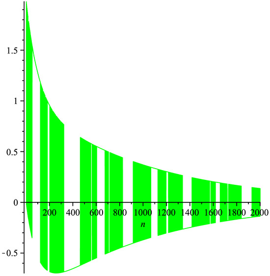
Figure 1.
Demonstration of the oscillatory behavior of the solution of (21) when n is large enough.
It can be seen from Figure 1 that the solution of Equation (21) is oscillatory in the case n is large enough.
Example 2.
According to (1), one has , .
We will use Theorem 2 to derive the oscillatory and asymptotic behaviour of Equation (22). To this end, it is necessary to verify (2), (9), (13), (14), (19), and (20). Obviously, (2), (9), (13), and (14) can be easily verified. On the other hand, for (19), if we let , and is defined as in Example 1, then one can obtain that
So furthermore one has
From the inequality above, one can deduce that (19) is satisfied. Moreover, if we let , then following in a similar manner as the analysis above, one can deduce that (20) is also satisfied. So, by using Theorem 2, the solution to Equation (22) is oscillatory or .
In (22), if we select the initial values as , then, it holds , which can be demonstrated in Figure 2.
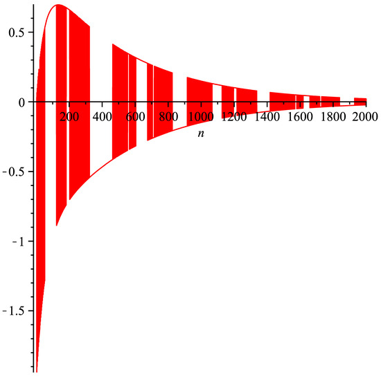
Figure 2.
Demonstration of the asymptotic behavior of the solution of (22) when n is large enough.
4. Conclusions
We have successfully established some oscillatory and asymptotic criteria for a fifth-order fractional difference equation through use of the Riccati transformation, inequality technique, and the properties of the conformable fractional difference and fractional sum. The process can be extended to other types of high-order fractional difference equations as well as fractional differential equations, such as fifth-order fractional differential or difference equations with a neutral term, damping term, or impulse term and so on, which is worthy for further research.
Funding
This research received no external funding.
Data Availability Statement
No new data were created or analyzed in this study. Data sharing is not applicable to this article.
Conflicts of Interest
The author declares no conflicts of interest.
References
- Sun, Y.; Zhao, Y. Oscillation criteria for third-order nonlinear neutral differential equations with distributed deviating arguments. Appl. Math. Lett. 2021, 111, 106600. [Google Scholar] [CrossRef]
- Šišoláková, J. Oscillation of linear and half-linear difference equations via modified Riccati transformation. J. Math. Anal. Appl. 2023, 528, 127526. [Google Scholar] [CrossRef]
- Chatzarakis, G.E.; Grace, S.R.; Jadlovská, I. On the sharp oscillation criteria for half-linear second-order differential equations with several delay arguments. Appl. Math. Comput. 2021, 397, 125915. [Google Scholar] [CrossRef]
- Attia, E.R.; Chatzarakis, G.E. Oscillation tests for difference equations with non-monotone retarded arguments. Appl. Math. Lett. 2022, 123, 107551. [Google Scholar] [CrossRef]
- Moaaz, O.; Ramos, H.; Awrejcewicz, J. Second-order Emden-Fowler neutral differential equations: A new precise criterion for oscillation. Appl. Math. Lett. 2021, 118, 107172. [Google Scholar] [CrossRef]
- Bohner, M.; Saker, S.H. Oscillation of second order nonlinear dynamic equations on time scales. Rocky Mt. J. Math. 2004, 34, 1239–1254. [Google Scholar] [CrossRef]
- Grace, S.R.; Agarwal, R.P.; Bohner, M.; O’Regan, D. Oscillation of second-order strongly superlinear and strongly sublinear dynamic equations. Commun. Nonlinear Sci. Numer. Simul. 2009, 14, 3463–3471. [Google Scholar] [CrossRef]
- Hassan, T.S.; Kong, Q. Oscillation criteria for higher-order nonlinear dynamic equations with Laplacians and a deviating argument on time scales. Math. Methods Appl. Sci. 2017, 40, 4028–4039. [Google Scholar] [CrossRef]
- Grace, S.R.; Negi, S.S.; Abbas, S. New oscillatory results for non-linear delay dynamic equations with super-linear neutral term. Appl. Math. Comput. 2022, 412, 126576. [Google Scholar] [CrossRef]
- Saker, S.H.; Sethi, A.K. Riccati technique and oscillation of second order nonlinear neutral delay dynamic equations. J. Comput. Anal. Appl. 2021, 29, 266–278. [Google Scholar]
- Feng, Q.; Zheng, B. Oscillation Criteria for Nonlinear Third-Order Delay Dynamic Equations on Time Scales Involving a Super-Linear Neutral Term. Fractal Fract. 2024, 8, 115. [Google Scholar] [CrossRef]
- Fečkan, M.; Danca, M.F.; Chen, G. Fractional Differential Equations with Impulsive Effects. Fractal Fract. 2024, 8, 500. [Google Scholar] [CrossRef]
- Kuzenov, V.V.; Ryzhkov, S.V. Developing a procedure for calculating physical processes in Combined Schemes of Plasma Magneto-Inertial Confinement. Bull. Russ. Acad. Sci. Phys. 2016, 80, 598–602. [Google Scholar] [CrossRef]
- Adiguzel, H. Oscillatory behavior of solutions of certain fractional difference equations. Adv. Differ. Equ. 2018, 2018, 445. [Google Scholar] [CrossRef]
- Abdalla, B. On the oscillation of q-fractional difference equations. Adv. Differ. Equ. 2017, 2017, 254. [Google Scholar] [CrossRef]
- Wang, Y.; Han, Z.; Zhao, P.; Sun, S. On the oscillation and asymptotic behavior for a kind of fractional differential equations. Adv. Differ. Equ. 2014, 2014, 50. [Google Scholar] [CrossRef]
- Chen, D.X. Oscillation criteria of fractional differential equations. Adv. Differ. Equ. 2012, 2012, 33. [Google Scholar] [CrossRef]
- Wang, Y.; Han, Z.; Sun, S. Comment on “On the oscillation of fractional-order delay differential equations with constant coefficients” [Commun Nonlinear Sci 19(11) (2014) 3988–3993]. Commun. Nonlinear Sci. Numer. Simulat. 2015, 26, 195–200. [Google Scholar] [CrossRef]
- Chatzarakis, G.E.; Elabbasy, E.M.; Bazighifan, O. An oscillation criterion in 4th-order neutral differential equations with a continuously distributed delay. Adv. Differ. Equ. 2019, 2019, 336. [Google Scholar] [CrossRef]
- Parhi, N.; Tripathy, A. On oscillatory fourth order linear neutral differential equations. I. Math. Slovaca 2004, 54, 389–410. [Google Scholar]
- Li, T.; Baculikova, B.; Dzurina, J.; Zhang, C. Oscillation of fourth order neutral differential equations with p-Laplacian like operators. Bound. Value Probl. 2014, 2014, 56. [Google Scholar] [CrossRef]
- Cesarano, C.; Bazighifan, O. Oscillation of fourth-order functional differential equations with distributed delay. Axioms 2019, 8, 61. [Google Scholar] [CrossRef]
- Moaaz, O.; Elabbasy, E.M.; Bazighifan, O. On the asymptotic behavior of fourth-order functional differential equations. Adv. Differ. Equ. 2017, 2017, 261. [Google Scholar] [CrossRef]
- Zhang, C.; Li, T.; Saker, S. Oscillation of fourth-order delay differential equations. J. Math. Sci. 2014, 201, 296–308. [Google Scholar] [CrossRef]
- Khalil, R.; Al-Horani, M.; Yousef, A.; Sababheh, M. A new definition of fractional derivative. J. Comput. Appl. Math. 2014, 264, 65–70. [Google Scholar] [CrossRef]
- Zhou, H.W.; Yang, S.; Zhang, S.Q. Conformable derivative approach to anomalous diffusion. Phys. A 2018, 491, 1001–1013. [Google Scholar] [CrossRef]
- Yang, S.; Wang, L.; Zhang, S. Conformable derivative: Application to non-Darcian flow in low-permeability porous media. Appl. Math. Lett. 2018, 79, 105–110. [Google Scholar] [CrossRef]
- Tasbozan, O.; Çenesiz, Y.; Kurt, A.; Baleanu, D. New analytical solutions for conformable fractional PDEs arising in mathematical physics by exp-function method. Open Phys. 2017, 15, 647–651. [Google Scholar] [CrossRef]


Disclaimer/Publisher’s Note: The statements, opinions and data contained in all publications are solely those of the individual author(s) and contributor(s) and not of MDPI and/or the editor(s). MDPI and/or the editor(s) disclaim responsibility for any injury to people or property resulting from any ideas, methods, instructions or products referred to in the content. |
© 2024 by the author. Licensee MDPI, Basel, Switzerland. This article is an open access article distributed under the terms and conditions of the Creative Commons Attribution (CC BY) license (https://creativecommons.org/licenses/by/4.0/).