Abstract
This paper investigates the explicit, accurate soliton and dynamic strategies in the resolution of the Wazwaz–Benjamin–Bona–Mahony (WBBM) equations. By exploiting the ensuing wave events, these equations find applications in fluid dynamics, ocean engineering, water wave mechanics, and scientific inquiry. The two main goals of the study are as follows: Firstly, using the dynamic perspective, examine the chaos, bifurcation, Lyapunov spectrum, Poincaré section, return map, power spectrum, sensitivity, fractal dimension, and other properties of the governing equation. Secondly, we use a generalized rational exponential function (GREF) technique to provide a large number of analytical solutions to nonlinear partial differential equations (NLPDEs) that have periodic, trigonometric, and hyperbolic properties. We examining the wave phenomena using 2D and 3D diagrams along with a projection of contour plots. Through the use of the computational program Mathematica, the research confirms the computed solutions to the WBBM equations.
1. Introduction
In many fields of physics, mathematics, and engineering, nonlinear partial differential equations (NLPDEs) has been used to investigate physical processes [,]. Analytical solutions of NLPDEs are crucial for predicting the dynamics of a physical process governed by these equations. Researchers have proposed several analytical techniques to extract analytical solutions of NLPDEs. Some of them are: the binary F-expansion method [], the modified Kudryashov scheme [], the Hirota bilinear technique [], the modified extended tanh-function technique [], the Khater technique [], the advanced expansion techniques [], the tanh-coth technique [], the variational iteration technique [], the technique of characteristics [], the modified Sardar sub equation technique [], the modified Fan sub-equation approach [], the modified rational sin-cos and sinh-cosh techniques [], the Darboux transformation technique [], the Bernoulli sub-ODE technique [], the improved -expansion technique [], the modified direct algebraic technique [], the improved Bernoulli sub-equation technique [], the complex technique [], the modified simple equation technique [], the Riccati Bernoulli sub ODE technique [], and so on [,,,].
Wazwaz provides a framework and generalization of multiple notions that have been used in the literature []. This unique structure is present in the (3+1)-dimensional BBM equations. This work aims to analyze the complex dynamics lying behind the WBBM equations
where are the spatial terms and t is a temporal term. There are several studies on WBBM equation in the literature [,,].
Chaos analysis has become interest of researchers, because it provides a deeper analysis of complex systems that appear disordered, but follow underlying patterns. Chaos theory has many profound applications in neural networks [,], biology [,], and physics [,]. Via chaos analysis, we can better explain real-world systems, enhance predictions, and develop more robust solutions to challenges in science, technology, and engineering. In NLPDEs, currently, chaos analysis has gained much interest of the mathematician and physicists. Soliton solutions and chaos analysis of different NLPDEs have been reported in the literature [,,,]. In this study, we aim to extract analytical solutions to the WBBM equation by applying the GREF technique []. In addition, sensitivity analysis to the governing equation, bifurcation analysis, and chaos analysis are all examined graphically.
The layout of the manuscript is as follows: In Section 2, analysis and graphical visualization of dynamic properties of governed equation are explored. In Section 3, we briefly describe the GREF technique. In Section 4, we implement the GREF technique to the governing equation to acquire the soliton solutions. In Section 5, a discussion on the obtained results is provided. The conclusion is provided in Section 6.
2. Dynamic System Governed from Proposed Equation
This section provides the transformation of proposed Equations (1)–(3) into the system of ODEs. First, we use wave transformation to convert the considered PDEs into the ODEs. After obtaining the ODE, it is converted into a system of ODEs with the help of Galilean transformation. So, we start by using the following:
where . After the insertion of Equation (4) in Equation (1), the following nonlinear ODE can be obtained:
It should be noted that when we substitute the proposed wave transform into Equations (2) and (3), we obtain the same results as after the substitution of the wave transformation into Equation (1). On performing the integration of Equation (5) concerning the only once, and supposing the constant of integration as zero, we obtain the result presented below:
Here, by making use of the Galilean transformation, Equation (6) gives rise to the following system of ODEs:
where
2.1. The Analysis and Graphical Visualizations of Chaos and Other Behaviors of Equation (7)
This section of the current research is focused on conducting a thorough examination and analysis of chaotic dynamics, sensitivity, and additional analysis pertaining to the suggested system of ODEs.
2.2. Chaos in the Proposed System
This section delves into the potential presence of chaos within the system described by Equation (7), through the incorporation of a perturbation term. This portion also analyzes the 2D and 2D vs. time phase diagrams of the governed system. After inserting the perturbation, we obtained the following:
In this part, Figure 1 and Figure 2 analyze the influences of the added term on the dynamic behavior of the proposed system (8). In the added term, means amplitude, while represents frequency of the proposed system.
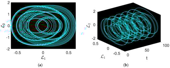
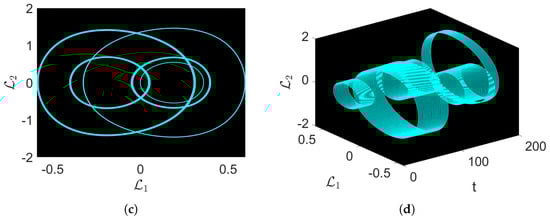
Figure 1.
Chaotic visual representations of a suggested equation, with the parameters taken into consideration as . (a) 2D dynamics of vs. for . (b) 3D dynamics of vs. vs. t for . (c) 2D dynamics of vs. for . (d) 3D dynamics of vs. vs. t for .
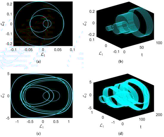
Figure 2.
Chaotic visual representations of a suggested equation, with the parameters taken into consideration as . (a) 2D graph for . (b) 3D dynamics for . (c) 2D behavior for . (d) 3D behavior for .
The 2D and 2D against-time phase images for the study of the underlying complex dynamics of the system are presented by the utilization of parameters in the form of , while varying the amplitudes and frequency, such that and are considered differently, as in Figure 1a,b and in Figure 1c,d. Further, in Figure 2, we consider for in Figure 2a,b, and in Figure 2c,d.
After analyzing the phase diagrams, captivating and complex dynamics are observed. In Figure 1a, multi-scroll torus-type dynamics are observed, while in Figure 1c, strange and complex dynamics can be seen. Moreover, in Figure 2a, complex multi-scroll torus-like behavior is observed, while Figure 2c shows complex torus-shaped oscillations. These observations reveal the system’s susceptibility to the added perturbations arising in , offering a substantial understanding of how the term impacts the overall behavior of the governed system. The newly discovered insights into the system’s susceptibility to parameter variations enhance our understanding of the intricate connections within and the system’s overall dynamics. These understandings further facilitate a wider comprehension of how small changes navigate the trajectories of the proposed dynamic system.
2.3. Effects of Parameters on the Chaotic Flow of the System
This section investigates the effects of parameters on the dynamics of the proposed system. Figure 3 displays six figures showcasing different chaotic structures. The figures are labeled according to variations in the parameters, specifically and , which influence the system’s chaotic dynamics. Figure 3a–c demonstrate the behavior with varying , while Figure 3d–f show the dynamics with varying . We will discuss each plot in more detail and analyze the effect of the proposed parameters on the chaotic structures. Figure 3a displays a structure resembling a figure-eight or a double-loop pattern. This indicates the presence of a chaotic attractor where the system’s state oscillates between the two loops. The loops are twisted together, suggesting a low level of chaos and a more periodic nature. When we consider (as observed in Figure 3b), the loops appear more separated compared to the previously simulated case, resulting in a simpler overall structure. This change in structure indicates a shift in the dynamics of the proposed system, potentially making the attractor less chaotic and more stable. Figure 3c simulates the system with , which shows a more complex structure with multiple coinciding loops. This indicates increased sophistication and greater chaos within the proposed system. The overlapping loops are indicative of a highly sensitive dependence on parameters, a defining characteristic of chaotic models. Figure 3d shows the impact of the parameter on the proposed model, displaying a tight, complex looping pattern. The large value of introduces higher oscillations in the model, contributing to the intricate pattern observed. The tight loops indicate a high level of chaotic and complex behavior. Further, in Figure 3e, the behavior is simpler and more symmetric on the axis compared to Figure 3d. This suggests that the dynamics exhibits less chaos at the value of . The symmetry indicates more regular and less chaotic behavior. Finally, in Figure 3f, is set to 0.90. The pattern observed in this simulation is more chaotic, featuring several overlapping loops. The small value of the parameter introduces slow oscillations, but the complexity indicates high sensitivity. The chaotic structure with overlapping loops is indicative of strong chaos within the system. These simulations demonstrate how small perturbations in system parameters can substantially change the system’s dynamics, a fundamental feature of chaotic systems. Each parameter affects the system in a completely different way, contributing to the overall behavior and complexity of the chaotic system.
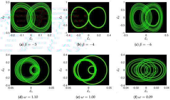
Figure 3.
Effects of parameters and on the behavior of the chaos on the governed system with other parameters supposed as . The 2D dynamics are depicted in subplots: (a) for (b) for and (c) for . The 2D dynamics are displayed in subplots: (d) for , (e) for and (f) for .
2.4. Some New Dynamic Properties of the Proposed Model
This portion of the manuscript is devoted to the analysis of several qualitative characteristics of the proposed system, ranging from bifurcation analysis to Lyapunov exponents (LEs), strange attractors, and more. Figure 4 illustrates the bifurcation behavior of the proposed model with respect to the parameter in both state variables and . Figure 4a specifically shows bifurcation in vs. . The figure depicts regions of unstable and stable behavior. At small values of , fewer points are observed, indicating limited or zero bifurcations. As increases, the system exhibits more complex dynamics with a wider spread of points, signifying a transition to chaos or the coexistence of multiple attractors. The gaps and dense clusters of points suggest periods of abrupt qualitative changes in the system’s behavior. The second diagram, Figure 4b, shows variations in vs. the parameter . The dynamics of the system in this simulation exhibits notable differences compared to Figure 4a. At low values of , distinct branches can be observed, indicating fixed points or stable periodic orbits. As increases, the branches begin to diverge and ultimately transition into more scattered behavior, indicating the onset of chaos. The spreading of points at larger values of suggests that the system evolves into increasingly complex dynamics, potentially with multiple attractors and a possible transition to chaos.
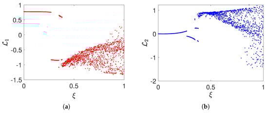
Figure 4.
Bifurcation in the proposed system, with the parameters taken into consideration as , . (a) Bifurcation of vs. . (b) Bifurcation of vs. .
Figure 5 illustrates the Lyapunov spectrum, Poincaré section (PS), return map, and power spectrum of the proposed model. Figure 5a demonstrates the dynamics of the two Lyapunov exponents (LEs) ( and ) versus time. Lyapunov exponents measure the rates of separation of infinitesimally close orbits within a dynamic system. In this figure, is positive, indicating that the system exhibits sensitive dependence on initial conditions, a hallmark of chaos. A positive LE confirms that even a small perturbation in the initial values will lead to exponentially divergent trajectories, rendering long-term prediction impossible. Conversely, has a negative value, signifying that some directions contract within the phase space. Figure 5b shows the Poincaré section (PS), which is a 2D slice of the system’s phase space region considered at fixed intervals. The observed spiral-shaped behavior indicates the presence of an intricate, multi-dimensional attractor. The recurrence, though not overlapping, suggests deterministic but aperiodic chaotic dynamics. The PS provides a clear view of the system’s dynamics, making it easier to visualize the behavior of a chaotic attractor. Figure 5c displays the return map, which depicts the relationship between the value of a variable at a certain time step () and its value at the next time step (). The concentrated, diagonal structure of the return map suggests a strong correlation between successive values, indicative of deterministic behavior with underlying chaotic dynamics. This map assists in understanding how the state of the system evolves over time, and can also highlight the periodic behavior and nature of attractors in lower-dimensional presentations. Finally, Figure 5d shows the power spectrum of the time series data from the proposed system, visualizing its frequency content. The presence of several peaks, especially at fractional multiples of the fundamental frequency, is representative of the broad spectrum typical of chaotic waves. The dominant low-frequency peaks suggest that the system exhibits long-term, complex-type oscillations. The power spectrum provides a frequency domain perspective of the system’s dynamics, complementing the time domain and phase space analyses.
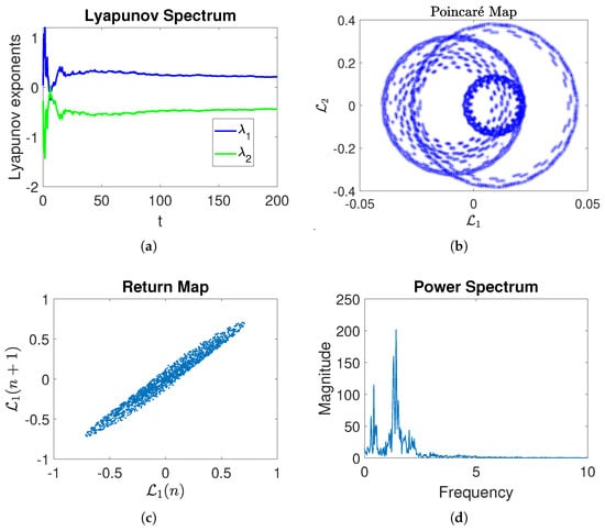
Figure 5.
Visual representations of different characteristics of the suggested equation, with the parameters taken into consideration as . (a) Lyapunov exponent vs. time. (b) Poincaré map of vs. . (c) Return map. (d) Power spectrum.
Figure 6 visualizes the dynamics of fractal dimension, recurrence plots, and strange attractors of the proposed system. The fractal dimension is a measure of how densely a fractal fills space as one zooms in to finer scales. In Figure 6a, the y-axis represents the counts of instances within various box indices on the x-axis. The irregular peaks and non-uniform dynamics indicate the complex structure of the system, revealing its fractal nature. The fractal dimension quantifies the complexity of the system, demonstrating that the attractor fills space in a self-similar and detailed manner across various scales. The recurrence plot, shown in Figure 6b, is used to demonstrate the recurrence and periodicity of states within the system over time. Time is represented on both axes, and the intensity of the color indicates the recurrence of repeating states. The diagonal forms and grid-like patterns reflect the system’s hidden periodicity and deterministic nature, while intricate patterns showcase the complex, recurrent behavior characteristic of chaotic systems. Recurrence plots depict the times at which a system returns to previous states, revealing both periodic and chaotic dynamics. Finally, the strange attractor of the proposed system is displayed in Figure 6c. This figure illustrates the trajectory of the proposed system by visualizing against and . The crowded, twisted layers and loops visualize the complexity of the chaotic attractor. The structure demonstrates that the system’s trajectory never intersects itself exactly, despite revolving through the same regions in phase space repeatedly.
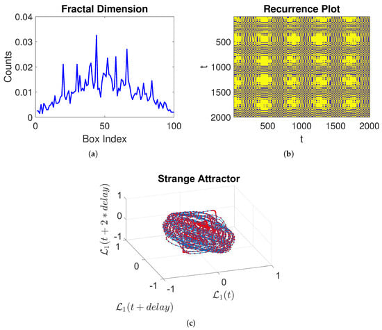
Figure 6.
Visual representation of different characteristics of the suggested equation, with the parameters taken into consideration as . (a) Fractal dimension (b) Recurrence plot (c) 3D dynamics of a strange attractor.
2.5. Sensitivity Analysis
Here, we simulate and analyze the sensitivity analysis of the proposed model, as observed in Equation (7). To do so, let us consider the dynamic model in the form of
The parameters for the simulations of the above system are assumed as , , while the initial conditions are used as follows: Blue curve: represents the dynamics of the governed system with . Green curves: show the oscillations in the proposed model with . Red curves: depict the system evolution with .
The results obtained from this analysis are illustrated in Figure 7. Observations of the figures indicate that minor perturbations in initial values lead to significant changes in the dynamics of the proposed system.
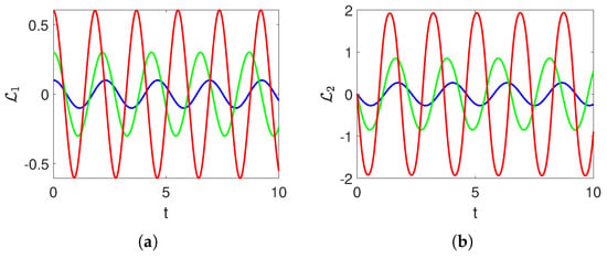
Figure 7.
Numerical simulations depicting the state variables over time, considering the parameters as with various initial values considered as . (a) Sensitivity of (b) Sensitivity of .
3. Mathematical Analysis of the GREF Technique
This is an overview of the GREF methodology that we use in our work.
- Step 1:From the WBBM equations, we obtain a nonlinear ordinary differential equation (NLODE) by applying the transformations defined in Equations (4) to (1)–(3).
- Step 2:
- Step 3:Calculating N by using the homogeneous balancing principle. To generate the following polynomial equation, insert NLODE into Equation (11) and gather all the terms.
- Step 4:Set each coefficient of m to zero, we obtained the set of the algebraic equation for and to be obtained.
- Step 5:Once the set of equations solved, the nontrivial solutions will be substituted into NLODE. As a result, the soliton solutions to Equations (1)–(3) will be obtained.
4. Implementation of the GREF Technique to the Governing Equation
To acquire the soliton solution, we apply the GREF technique to Equation (6) in this section. is the result of solving Equation (6) using the homogeneous balancing principle. Using the GERF technique, we obtain the analytical solutions in the form as
By equating all of the coefficients to zero and inserting Equation (13) into Equation (6) using Equation (10), we are left with an algebraic system of equations. The family of solutions obtained by applying the system of algebraic equations is as follows:
- Family i:and ; then, Equation (10) revealsCluster 1:then, we obtainCluster 2:then, we obtainCluster 3:then, we obtainCluster 4:then, we obtainCluster 5:then, we obtainCluster 6:then, we obtain
- Family ii:; then, Equation (10) revealsCluster 1:then, we obtainCluster 2:then, we obtainCluster 3:then, we obtainCluster 4:then, we obtainCluster 5:then, we obtainCluster 6:then, we obtain
5. Results and Discussion
Using a variety of mathematical tools, including the GREF technique, bifurcation analysis, chaos analysis, and sensitivity analysis, we examined the behavior of the WBBM equation, and developed numerous solutions. The WBBM equation contains multiple different types of solutions, including periodic, kink, and anti-kink solutions, according to our research. These solutions are crucial, because they demonstrate the WBBM equation’s nonlinear behavior and help scholars understand how the equation might be used in a range of fields, such as mathematics, physics, and engineering. Soliton wave packets are stable, and localized within nonlinear systems. They play a significant role in various fields, particularly in explaining the behavior of nonlinear partial differential equations (NPDEs). The existence of infinite soliton solutions in NPDEs provides insights into the underlying nonlinear dynamics. Studying these solutions is particularly interesting for applications such as optical communications, as they offer insights into how energy propagates throughout the system and how nonlinear dynamics and localized heat distributions behave. The fields of information transmission, nonlinear systems, and heat transfer can all benefit from these solutions. Periodic solutions are useful for understanding stability, oscillatory properties, and the long-term behavior of wave propagation processes. The periodic wave solution of is shown in Figure 8. Figure 9 represents the interaction of a kink soliton with a lump soliton, which is expressed . The periodic lump soliton solution of is shown in Figure 10. Another periodic solution of is shown in Figure 11. This technique offers physicists and mathematicians an innovative approach to understanding the physical properties of phenomena that occur in nature. The technique is reliable, effective, and concise, proving valuable for addressing NLPDEs in various research fields. The numerical and exact results appear to align, encouraging further investigation into the proposed equation. Our discoveries have applications in several fields of mathematics, physics, and other scientific disciplines.
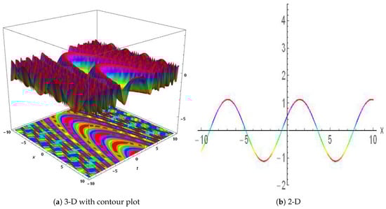
Figure 8.
Physical depiction of Equation (15), of at , and . (a) 3D dynamics of the . (b) 2D dynamics of the .
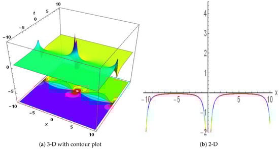
Figure 9.
Physical depiction of Equation (17), of at , and . (a) 3D dynamics of the . (b) 2D dynamics of the .
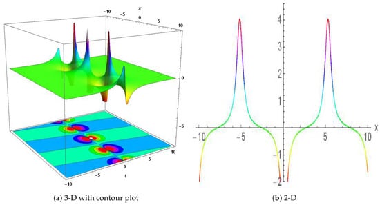
Figure 10.
Physical depiction of Equation (19), of at , and . (a) 3D dynamics of the . (b) 2D dynamics of the .
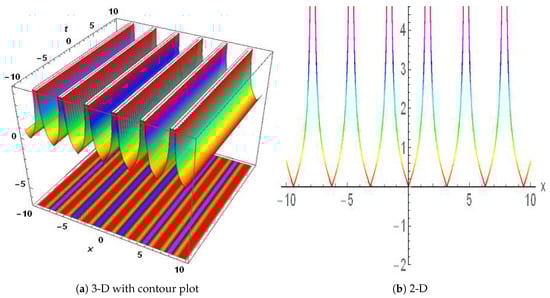
Figure 11.
Physical depiction of Equation (24), of at , and . (a) 3D dynamics of the . (b) 2D dynamics of the .
6. Conclusions
This current research work successfully investigated the (3+1)-dimensional WBBM equation by employing a variety of techniques. These techniques have played a significant role in many fields, such as fluid dynamics, ocean engineering, water wave mechanics, and scientific research, where a thorough understanding of wave phenomena is crucial. To obtain novel solutions, we employed the generalized rational exponential functions technique to generate analytical solutions with periodic, trigonometric, and hyperbolic characteristics.
Furthermore, we analyzed the dynamic behavior of the system, examining chaos, bifurcation, Lyapunov spectrum, Poincaré section, return map, power spectrum, sensitivity, fractal dimension, and other properties. The results were effectively illustrated through 2D and 3D plots, including contour plots, to demonstrate the significance of wave propagation. The paper highlights the usefulness of the suggested technique in producing precise solutions for nonlinear partial differential equations (NLPDEs), and underscores its importance for engineering and research applications by comparing its findings with those of previous studies.
The potential usefulness of these solutions in developing nonlinear water models for ocean and coastal engineering applications is demonstrated through the validation of computed solutions using Mathematica. The paper contains multiple soliton solutions, such as periodic solitons, lump solitons, etc. The periodic solitons are essential in the design of breakwater or piers. The periodic soliton can give information on the stability and flexibility of these patterns under changing wave conditions. Lump solitons play key role in coastal engineering. Lump solitons discuss cases where lump solitons have been utilized to study wave packets in coastal water, such as the formation of wave group that can influence sludge transport or cause sudden loading on offshore platforms. Overall, this work enhances our understanding of, and skill in handling, WBBM equations in a variety of real-world contexts. It provides insightful information for future research and applications in related domains.
Author Contributions
Conceptualization, M.S.; Software, A.M.; Formal analysis, M.S.; Investigation, M.S. and A.A.; Writing—original draft, K.A.; Writing—review and editing, A.E.H., A.A. and H.S.; Funding acquisition, A.E.H. All authors have read and agreed to the published version of the manuscript.
Funding
This research received no external funding.
Data Availability Statement
No data were used in this paper.
Acknowledgments
The Researchers would like to thank the Deanship of Graduate Studies and Scientific Research at Qassim University for financial support (QU-APC-2024-9/1).
Conflicts of Interest
The authors declare no conflicts of interest.
Correction Statement
This artcle has been republished with a minor correction to the Acknowledgement part. This change does not affect the scientific content of the article.
References
- Lokenath, D.; Debnath, L. Nonlinear Partial Differential Equations for Scientists and Engineers; Birkhäuser: Boston, MA, USA, 2005. [Google Scholar]
- Maziar, R.; Karniadakis, G.E. Hidden physics models: Machine learning of nonlinear partial differential equations. J. Comput. Phys. 2018, 357, 125–141. [Google Scholar]
- Rui, W.; He, B.; Long, Y. The binary F-expansion method and its application for solving the (n+1)-dimensional sine-Gordon equation. Commun. Nonlinear Sci. Numer. Simul. 2009, 14, 1245–1258. [Google Scholar] [CrossRef]
- Kumar, D.; Seadawy, A.R.; Joardar, A.K. Modified Kudryashov method via new exact solutions for some conformable fractional differential equations arising in mathematical biology. Chin. J. Phys. 2018, 56, 75–85. [Google Scholar] [CrossRef]
- Saifullah, S.; Ahmad, S.; Alyami, M.A.; Inc, M. Analysis of interaction of lump solutions with kink-soliton solutions of the generalized perturbed KdV equation using Hirota-bilinear approach. Phys. Lett. A 2022, 454, 128503. [Google Scholar] [CrossRef]
- Abdou, M.A.; Soliman, A.A. Modified extended tanh-function method and its application on nonlinear physical equations. Phys. Lett. A 2006, 353, 487–492. [Google Scholar] [CrossRef]
- Khater, M.M.A.; Akinyemi, L.; Elagan, S.K.; El-Shorbagy, M.A.; Alfalqi, S.H.; Alzaidi, J.F.; Alshehri, N.A. Bright–dark soliton waves’ dynamics in pseudo spherical surfaces through the nonlinear Kaup–Kupershmidt equation. Symmetry 2021, 13, 963. [Google Scholar] [CrossRef]
- Mawa, H.Z.M.; Islam, S.M.R.; Bashar, M.H.; Roshid, M.M.; Islam, J.; Rahman, M.M.; Akter, S. Analytical Soliton Solutions and Wave Profiles for the Ba Model and the (3+1)-Dimensional Kp Equation by Using an Advanced-Expansion Scheme. Available online: https://ssrn.com/abstract=4541425 (accessed on 13 September 2024).
- Al-Mamun, A.; Ananna, S.N.; An, T.; Asaduzzaman, M.; Munnu Miah, M. Solitary wave structures of a family of 3D fractional WBBM equation via the tanh–coth approach. Partial. Differ. Equ. Appl. Math. 2022, 5, 100237. [Google Scholar] [CrossRef]
- Arife, A.S. The modified variational iteration transform method (MVITM) for solve non linear partial differential equation (NLPDE). World Appl. Sci. J. 2011, 12, 2274–2278. [Google Scholar]
- Mhadhbi, N.; Gana, S.; Alsaeedi, M.F. Exact solutions for nonlinear partial differential equations via a fusion of classical methods and innovative approaches. Sci. Rep. 2024, 14, 6443. [Google Scholar] [CrossRef]
- Khan, M.I.; Farooq, A.; Nisar, K.S.; Shah, N.A. Unveiling new exact solutions of the unstable nonlinear Schrödinger equation using the improved modified Sardar sub-equation method. Results Phys. 2024, 59, 107593. [Google Scholar] [CrossRef]
- Yomba, E. The extended fan sub-equation method and its application to the (2 + 1)-dimensional dispersive long wave and Whitham-Broer-Kaup equations. Chin. J. Phys. 2005, 43, 789–805. [Google Scholar]
- Cinar, M.; Onder, I.; Secer, A.; Yusuf, A.; Sulaiman, T.A.; Bayram, M.; Aydin, H. Soliton Solutions of (2 + 1)(2 + 1) Dimensional Heisenberg Ferromagnetic Spin Equation by the Extended Rational sine-cosine sine-cosine and sinh-cosh sinh-cosh Method. Int. J. Appl. Comput. Math. 2021, 7, 135. [Google Scholar] [CrossRef]
- Ali, A.; Ahmad, J.; Javed, S. Dynamic investigation to the generalized Yu–Toda–Sasa–Fukuyama equation using Darboux transformation. Opt. Quantum Electron. 2024, 56, 166. [Google Scholar] [CrossRef]
- Yang, X.-F.; Deng, Z.-C.; Wei, Y. A Riccati-Bernoulli sub-ODE method for nonlinear partial differential equations and its application. Adv. Diff. Equations 2015, 2015, 117. [Google Scholar] [CrossRef]
- Kadkhoda, N.; Jafari, H. Analytical solutions of the Gerdjikov–Ivanov equation by using exp-(ϕ(ξ))-expansion method. Optik 2017, 139, 72–76. [Google Scholar] [CrossRef]
- Yasin, S.; Khan, M.A.; Ahmad, S.; Aldosary, S.F. Abundant new optical solitary waves of paraxial wave dynamical model with kerr media via new extended direct algebraic method. Opt. Quantum Electron. 2024, 56, 925. [Google Scholar] [CrossRef]
- Ibrahim, S. Optical soliton solutions for the nonlinear third-order partial differential equation. Adv. Differ. Equations Control. Process. 2022, 29, 127–138. [Google Scholar] [CrossRef]
- Xia, Y.; He, Y.; Wang, K.; Pei, W.; Blazic, Z.; Mandic, D.P. A complex least squares enhanced smart DFT technique for power system frequency estimation. IEEE Trans. Power Deliv. 2015, 32, 1270–1278. [Google Scholar] [CrossRef]
- Al-Amr, M.O. Exact solutions of the generalized (2 + 1)-dimensional nonlinear evolution equations via the modified simple equation method. Comput. Math. Appl. 2015, 69, 390–397. [Google Scholar] [CrossRef]
- Ahmed, M.S.; Zaghrout, A.A.; Ahmed, H.M. Travelling wave solutions for the doubly dispersive equation using improved modified extended tanh-function method. Alex. Eng. J. 2022, 61, 7987–7994. [Google Scholar] [CrossRef]
- Ali, S.; Ullah, A.; Aldosary, S.F.; Ahmad, S.; Ahmad, S. Construction of optical solitary wave solutions and their propagation for Kuralay system using tanh-coth and energy balance method. Results Phys. 2024, 59, 107556. [Google Scholar] [CrossRef]
- Ali, S.; Ahmad, J.; Javed, S. Solitary wave solutions for the originating waves that propagate of the fractional Wazwaz-Benjamin-Bona-Mahony system. Alex. Eng. J. 2023, 69, 121–133. [Google Scholar] [CrossRef]
- Javed, S.; Ali, A.; Ahmad, J.; Hussain, R. Study the dynamic behavior of bifurcation, chaos, time series analysis and soliton solutions to a Hirota model. Opt. Quantum Electron. 2023, 55, 1114. [Google Scholar] [CrossRef]
- Ahmad, S.; Aldosary, S.F.; Khan, M.A.; Rahman, M.U.; Alsharif, F.; Ahmad, S. Analyzing optical solitons in the generalized unstable NLSE in dispersive media. Optik 2024, 307, 171830. [Google Scholar] [CrossRef]
- Wazwaz, A.-M. Exact soliton and kink solutions for new (3 + 1)-dimensional nonlinear modified equations of wave propagation. Open Eng. 2017, 7, 169–174. [Google Scholar] [CrossRef]
- Abbas, N.; Bibi, F.; Hussain, A.; Ibrahim, T.F.; Dawood, A.A.; Birkea, F.M.O.; Hassan, A.M. Optimal system, invariant solutions and dynamics of the solitons for the Wazwaz Benjamin Bona Mahony equation. Alex. Eng. J. 2024, 91, 429–441. [Google Scholar] [CrossRef]
- Abdulla-Al, M.; Shahen, N.H.M.; Ananna, S.N.; Asaduzzaman, M. Solitary and periodic wave solutions to the family of new 3D fractional WBBM equations in mathematical physics. Heliyon 2021, 7, e07483. [Google Scholar]
- Xu, C.; Zhao, Y.; Lin, J.; Pang, Y.; Liu, Z.; Shen, J.; Liao, M.; Li, P.; Qin, Y. Bifurcation investigation and control scheme of fractional neural networks owning multiple delays. Comput. Appl. Math. 2024, 43, 1–33. [Google Scholar] [CrossRef]
- Xu, C.; Lin, J.; Zhao, Y.; Cui, Q.; Ou, W.; Pang, Y.; Liu, Z.; Liao, M.; Li, P. New results on bifurcation for fractional-order octonion-valued neural networks involving delays. Netw. Comput. Neural Syst. 2024, 1–53. [Google Scholar] [CrossRef]
- Xu, C.; Ou, W.; Cui, Q.; Pang, Y.; Liao, M.; Shen, J.; Baber, M.Z.; Maharajan, C.; Ghosh, U. Theoretical exploration and controller design of bifurcation in a plankton population dynamical system accompanying delay. Discret. Contin. Dyn. Syst.-S 2024. [Google Scholar] [CrossRef]
- Xu, C.; Farman, M.; Shehzad, A. Analysis and chaotic behavior of a fish farming model with singular and non-singular kernel. Int. J. Biomath. 2023, 2350105. [Google Scholar] [CrossRef]
- Iskakova, K.; Alam, M.M.; Ahmad, S.; Saifullah, S.; Akgül, A.; Yılmaz, G. Dynamical study of a novel 4D hyperchaotic system: An integer and fractional order analysis. Math. Comput. Simul. 2023, 208, 219–245. [Google Scholar] [CrossRef]
- Lin, H.; Deng, X.; Yu, F.; Sun, Y. Diversified Butterfly Attractors of Memristive HNN with Two Memristive Systems and Application in IoMT for Privacy Protection. IEEE Trans. Comput. Des. Integr. Circuits Syst. 2024. [Google Scholar] [CrossRef]
- Ahmad, S.; Lou, J.; Khan, M.A.; Rahman, M.U. Analysing the Landau-Ginzburg-Higgs equation in the light of superconductivity and drift cyclotron waves: Bifurcation, chaos and solitons. Phys. Scr. 2023, 99, 015249. [Google Scholar] [CrossRef]
- Li, P.; Shi, S.; Xu, C.; Rahman, M.U. Bifurcations, chaotic behavior, sensitivity analysis and new optical solitons solutions of Sasa-Satsuma equation. Nonlinear Dyn. 2024, 112, 7405–7415. [Google Scholar] [CrossRef]
- Khan, A.; Saifullah, S.; Ahmad, S.; Khan, M.A.; Rahman, M.U. Dynamical properties and new optical soliton solutions of a generalized nonlinear Schrödinger equation. Eur. Phys. J. Plus 2023, 138, 1059. [Google Scholar] [CrossRef]
- Chahlaoui, Y.; Ali, A.; Ahmad, J.; Javed, S. Dynamical behavior of chaos, bifurcation analysis and soliton solutions to a Konno-Onno model. PLoS ONE 2023, 18, e0291197. [Google Scholar] [CrossRef]
- Ghanbari, B.; Inc, M. A new generalized exponential rational function method to find exact special solutions for the resonance nonlinear Schrödinger equation. Eur. Phys. J. Plus 2018, 133, 142. [Google Scholar] [CrossRef]
Disclaimer/Publisher’s Note: The statements, opinions and data contained in all publications are solely those of the individual author(s) and contributor(s) and not of MDPI and/or the editor(s). MDPI and/or the editor(s) disclaim responsibility for any injury to people or property resulting from any ideas, methods, instructions or products referred to in the content. |
© 2024 by the authors. Licensee MDPI, Basel, Switzerland. This article is an open access article distributed under the terms and conditions of the Creative Commons Attribution (CC BY) license (https://creativecommons.org/licenses/by/4.0/).