Computational and Numerical Analysis of the Caputo-Type Fractional Nonlinear Dynamical Systems via Novel Transform

Abstract

Two new methods for handling a system of nonlinear fractional differential equations are presented in this investigation. Based on the characteristics of fractional calculus, the Caputo fractional partial derivative provides an easy way to determine the approximate solution for systems of nonlinear fractional differential equations. These methods provide a convergent series solution by using simple steps and symbolic computation. Several graphical representations and tables provide numerical simulations of the results, which demonstrate the effectiveness and dependability of the current schemes in locating the numerical solutions of coupled systems of fractional nonlinear differential equations. By comparing the numerical solutions of the systems under study with the accurate results in situations when a known solution exists, the viability and dependability of the suggested methodologies are clearly depicted. Additionally, we compared our results with those of the homotopy decomposition method, the natural decomposition method, and the modified Mittag-Leffler function method. It is clear from the comparison that our techniques yield better results than other approaches. The numerical results show that an accurate, reliable, and efficient approximation can be obtained with a minimal number of terms. We demonstrated that our methods for fractional models are straightforward and accurate, and researchers can apply these methods to tackle a range of issues. These methods also make clear how to use fractal calculus in real life. Furthermore, the results of this study support the value and significance of fractional operators in real-world applications.

1. Introduction

Numerous academics have demonstrated the benefit of fractional calculus (FC) in generating specific solutions for an extensive number of linear and nonlinear partial differential equations in a number of recent articles. The creation of models and solutions for various physical problems are the primary goals of scientific efforts in engineering and physics. A foundation for the generalisation of differentiation to non-integer orders is provided by FC theory. An appropriate explanation of modelling problems including the ideas of non-locality and memory effect that cannot be sufficiently provided by integer-order operators is given by the fractional derivative operators [1,2]. FC defines physical phenomena more aggressively and precisely than classical calculus. Fractional calculus has gained significant attention in recent times. Fractional order nonlinear models are extensively employed in several domains and hold significance in nonlinear wave phenomena [3,4]. Many well-known mathematicians have made contributions to this topic in different works by suggesting an extensive number of fractional operators. FC frequently yields findings that are noticeably more accurate than those from classical calculus. It has demonstrated how several real-world scenarios behave dynamically among two integers. Furthermore, fractional operators possess more dimensions in comparison with integer differential operators. Notable fractional derivative formulations include those of Caputo [5], Miller [6], Riemann–Liouville [7], Caputo–Fabrizio [8], and Atangana–Baleanu [9]. Additionally, in this field of study, the Liouville–Caputo is regarded as the best fractional filter. Furthermore, we are aware that a wide range of non-local real-world phenomena that depend upon previous interactions are described by the Caputo fractional derivative. They have been applied in many different fields, including biology [10], nanotechnology [11], electrodynamics [12], chaos theory [13], biotechnology [14], continuum mechanics [15], and many more [16,17,18,19].

The majority of real-world problems are too complex to be modelled without the use of nonlinear fractional differential equations (NFDEs). NFDEs are therefore quite important in the present era. Numerous fields, including engineering, economics, ecology, and mathematical biology, have used NFDEs [20]. It is noteworthy that the mathematical sciences, which are regarded as the most interesting and demanding fields of study, present difficulties in developing the precise and explicit solutions to NFDEs. NFDEs can be broadly divided into two categories: integrable and non-integrable components. However, a significant number of nonlinear problems are difficult to solving analytically, and thus this development is insufficient due to the fact that NFDEs of both types cannot be solved exactly using any one technique [21]. Over the past few decades, work has been carried out in developing approaches for finding precise solutions to NFDEs. Many approaches are employed, but, depending on the problem’s nature, the researcher’s background, and the observatory context, each approach has benefits and drawbacks. Furthermore, the strategies employed to achieve this goal are always problem-specific. For this reason, some of these techniques are excellent when applied to specific issues but not when applied to others. Integral transformations have been identified as one of the most useful and effective methods in applied mathematics for resolving this problem. Many academics have developed and used a variety of strategies in recent years to find solutions for differential equations with fractional orders, such as the Yang transform decomposition method [22,23], exp-function algorithm [24], homotopy analysis transform method [25], natural transform decomposition method [26,27], finite element method [28], fractional residue power series method [29], finite difference and meshfree techniques [30], optimal homotopy asymptotic technique [31], radial basis functions and finite difference method [32], reduce differential transform method [33], Adams–Bashforth–Moulton method [34] and many more [35,36,37,38].

In this paper, we provide two new methods for the solving nonlinear fractional KdV system and nonlinear fractional dispersive long wave system of the following structures:

$$\begin{array}{cc}\hfill & D_{\mathrm{t}}^{{\delta }_i}{\mathrm{f}}_i(\mathrm{x},\mathrm{t})={\mathrm{j}}_i(\mathrm{x},\mathrm{t})+{\mathrm{L}}_i{\mathrm{f}}_i(\mathrm{x},\mathrm{t})+{\mathrm{N}}_i{\mathrm{f}}_i(\mathrm{x},\mathrm{t}),m_i-1\le {\delta }_i\le m_i\in N,i=1,2,\cdots ,n,\hfill \\ \hfill & {\displaystyle \frac{{\partial }^{k_i}{\mathrm{f}}_i}{\partial {\mathrm{t}}^{k_i}}}(\mathrm{x},0)={\mathrm{j}}_{i{k}_i}\left(\mathrm{x}\right),k_i=0,1,2,\cdots ,m_i-1,i=1,2,\cdots ,n,\hfill \end{array}$$

(1)

where ${\mathrm{L}}_i$ and ${\mathrm{N}}_i$ are linear and nonlinear operators, respectively, of $\mathrm{f}=\mathrm{f}(\mathrm{x},\mathrm{t})$ and its derivatives, which may contain other fractional derivatives of orders less than ${\delta }_i$, ${\mathrm{j}}_i(\mathrm{x},\mathrm{t})$ are known analytic functions, and $D_{\mathrm{t}}^{{\delta }_i}$ indicates the Caputo fractional derivative of order ${\delta }_i$. The system (1) assumes the homogeneous form when ${\mathrm{j}}_i(\mathrm{x},\mathrm{t})=0$. “Korteweg” and “de Vries” developed a dimensionless version of the equations for the study of dispersive wave occurrences in quantum mechanics and plasma physics called the (KdV) equation. The classic KdV equation was created in 1895 by Korteweg and de Vries as a nonlinear partial differential equation to model waves on the surface of shallow water. This particular solvable model has been the subject of numerous research studies. Recently, many scholars have suggested new applications of the classical KdV equation, such as representing acoustic waves on a crystal lattice, ion-acoustic waves in a plasma, and long internal waves in a density-stratified ocean. Boiti et al. [39] first suggested the classical long wave dispersive system, which explained the dynamical behaviours of nonlinear and dispersive long gravity waves in two horizontal directions on shallow waters of uniform depth. Numerous investigations have focused on this classical system because integer-order equations have strong integrability.

The Elzaki transform decomposition method (ETDM) and the homotopy perturbation transform method (HPTM) are two unique approaches that have been examined in this work. Tarig Elzaki developed the Elzaki transform, which greatly simplifies the time domain solution of ordinary and partial differential equations. Adomian has been working on a numerical method of solving functional equations since the 1980s [40,41]. It provides analysis in the form of a rapidly converging series that leads to the precise solutions. It is regarded as a potent technique for handling partial and differential equations of both integer and non-integer order, that are linear and nonlinear, homogeneous and nonhomogeneous. He first proposed the homotopy perturbation method (HPM) in 1998 [42], and it leads to a very quick convergence solution in the form of a series [43,44]. In summary, the original fractional partial differential equation (FPDE) is converted into its corresponding partial differential equation (PDE) by approximating the Caputo-type temporal fractional derivative using the Elzaki transform approach. The initial FPDE can be easily and quickly solved by using the homotopy perturbation approach and the Adomian decomposition method to the resulting PDE. As a useful and efficient mathematical tool for solving nonlinear equations, it usually only requires one iteration to produce a highly precise solution. Researchers can use this study as a primary reference to investigate these methodologies and use it in many applications to acquire accurate and approximate outcomes in a few easy steps. Our techniques provide infinite series as a result in the numerical cases. When expressed in closed form, the series offers a precise solution to the associated equations. The suggested techniques provide a high degree of accuracy at a low computational cost.

The structure of this research study is as follows. Section 1 of the paper contains the article’s introduction and goal. In Section 2 and Section 3, the basic ideas of fractional calculus are discussed. In Section 4 and Section 5, we present an overview of the proposed methodologies. Section 6 covers the convergence analysis of the proposed methods. A few numerical examples are shown in Section 7 to demonstrate the effectiveness of the proposed solutions. Section 8 presents the conclusion of the manuscript.

2. Basic Concept

In this part, we are going to provide some fundamental ideas, definitions, and characteristics of FC related to present work.

Definition 1.

The Caputo fractional derivative is defined as [45,46,47]

$$D^{\delta }f\left(x\right)=\left\{\begin{array}{c}{\displaystyle \frac{1}{\mathsf{\Gamma }(n-\delta )}}{\int }_0^x{\displaystyle \frac{f^n\left(t\right)}{{(x-t)}^{\delta -n+1}}}dt,n-1<\delta <n,\hfill \\ {\displaystyle \frac{d^n}{d{x}^n}}f\left(x\right),n=\delta .\hfill \end{array}\right.$$

(2)

with properties

$$\begin{array}{cc}\hfill J_t^{\delta }{D}_x^{\delta }g\left(t\right)& =g\left(t\right)-\sum _{k=0}^m{g}^k\left(0^{+}\right){\displaystyle \frac{t^k}{k!}},fort>0,andn-1<\delta \le n,n\in N.\hfill \\ \hfill D_t^{\delta }{J}_t^{\delta }g\left(t\right)& =g\left(t\right).\hfill \end{array}$$

(3)

Definition 2.

The Riemann–Liouville (RL) fractional derivative is defined as [45,46,47]

$$D^{\delta }f\left(x\right)=\left\{\begin{array}{c}{\displaystyle \frac{d^n}{d{x}^n}}f\left(x\right),\delta =n,\hfill \\ {\displaystyle \frac{1}{\mathsf{\Gamma }(n-\delta )}}{\displaystyle \frac{d}{d{x}^n}}{\int }_0^x{\displaystyle \frac{f\left(t\right)}{{(x-t)}^{\delta -n+1}}}dt,n-1<\delta <n,\hfill \end{array}\right.$$

(4)

with $n\in Z^{+}$, $\delta \in R^{+}$, and

$$D^{-\delta }f\left(x\right)={\displaystyle \frac{1}{\mathsf{\Gamma }\left(\delta \right)}}{\int }_0^x{(x-t)}^{\delta -1}f\left(t\right)dt,0<\delta \le 1.$$

(5)

Definition 3.

The RL fractional integral is defined as [45,46,47]

$$J^{\delta }f\left(x\right)={\displaystyle \frac{1}{\mathsf{\Gamma }\left(\delta \right)}}{\int }_0^x{(x-t)}^{\delta -1}f\left(t\right)dt,t>0,\delta >0.$$

(6)

with properties

$$\begin{array}{c}\hfill J^{\delta }{t}^n={\displaystyle \frac{\mathsf{\Gamma }(n+1)}{\mathsf{\Gamma }(n+\delta +1)}}{t}^{n+\delta },\\ \hfill D^{\delta }{t}^n={\displaystyle \frac{\mathsf{\Gamma }(n+1)}{\mathsf{\Gamma }(n-\delta +1)}}{t}^{n-\delta }.\end{array}$$

(7)

3. Elzaki Transform (ET)

Definition 4.

The Elzaki transform (ET) of $f\left(t\right)$ is defined as [48]

$$\mathtt{E}\left\{f\left(t\right)\right\}=M\left(u\right)=u{\int }_0^{\infty }{e}^{{\displaystyle \frac{-t}{u}}}f\left(t\right)dt,t>0,$$

(8)

with u indicating the transform variable.

We may obtain the ET of partial derivatives by utilising integration by parts in Equation (8) as below:

• ${\displaystyle \mathtt{E}\left[{\mathrm{t}}^n\right]=n!u^{n+2}.}$
• ${\displaystyle \mathtt{E}\left[{\mathrm{f}}^{\prime }\right]=\frac{M\left(u\right)}{u}-u\mathrm{f}\left(0\right).}$
• ${\displaystyle \mathtt{E}\left[{\mathrm{f}}^{″}\right]=\frac{M\left(u\right)}{u^2}-\mathrm{f}\left(0\right)-u{\mathrm{f}}^{\prime }\left(0\right).}$
• ${\displaystyle E\left[{\mathrm{f}}^n\right]=\frac{M\left(u\right)}{u^2}-\sum _{i=0}^{n-1}{u}^{2-n+i}{\mathrm{f}}^{\left(i\right)}\left(0\right).}$

ET of Caputo Fractional Derivative

Theorem 1.

If $\mathbf{J}\left(s\right)$ is the Laplace transform of $f\left(t\right)$, then ET $M\left(u\right)$ of $f\left(t\right)$ is given by [49]

$$M\left(u\right)=u\mathbf{J}\left({\displaystyle \frac{1}{u}}\right).$$

(9)

Theorem 2.

Let $M\left(u\right)$ be the ET of the function f(t), then [49]

$$\mathtt{E}\left[D_x^{\delta }f\left(x\right)\right]=u^{-\delta }\mathtt{E}\left[f\left(x\right)\right]-\sum _{i=0}^{n-1}{u}^{2-\delta +i}{f}^{\left(i\right)}\left(0\right),wheren-1<\delta <n.$$

(10)

4. Analysis of the HPTM

In order to better understand the fundamental concept and algorithm of the HPTM, we examine the below general nonlinear fractional model:

$$D_{\mathrm{t}}^{\delta }\mathrm{f}(\mathrm{x},\mathrm{t})=\mathrm{L}\left[\mathrm{x}\right]\mathrm{f}(\mathrm{x},\mathrm{t})+\mathrm{N}\left[\mathrm{x}\right]\mathrm{f}(\mathrm{x},\mathrm{t}),0<\delta \le 1,$$

(11)

with

$$\mathrm{f}(\mathrm{x},0)=\xi \left(\mathrm{x}\right).$$

Here, $D_{\mathrm{t}}^{\delta }={\displaystyle \frac{{\partial }^{\delta }}{\partial {\mathrm{t}}^{\delta }}}$ indicates the Caputo fractional operator, $\mathrm{L}\left[\mathrm{x}\right]$ is linear, and $\mathrm{N}\left[\mathrm{x}\right]$ is a nonlinear operator.

Executing the ET, we have

$$\mathtt{E}\left[D_{\mathrm{t}}^{\delta }\mathrm{f}(\mathrm{x},\mathrm{t})\right]=\mathtt{E}[\mathrm{L}\left[\mathrm{x}\right]\mathrm{f}(\mathrm{x},\mathrm{t})+\mathrm{N}\left[\mathrm{x}\right]\mathrm{f}(\mathrm{x},\mathrm{t})],$$

(12)

$${\displaystyle \frac{1}{u^{\delta }}}\{M\left(u\right)-u^2\mathrm{f}\left(0\right)\}=\mathtt{E}[\mathrm{L}\left[\mathrm{x}\right]\mathrm{f}(\mathrm{x},\mathrm{t})+\mathrm{N}\left[\mathrm{x}\right]\mathrm{f}(\mathrm{x},\mathrm{t})].$$

(13)

Thus we obtain

$$M\left(u\right)=u^2\mathrm{f}\left(0\right)+u^{\delta }\mathtt{E}[\mathrm{L}\left[\mathrm{x}\right]\mathrm{f}(\mathrm{x},\mathrm{t})+\mathrm{N}\left[\mathrm{x}\right]\mathrm{f}(\mathrm{x},\mathrm{t})].$$

(14)

Executing the inverse ET, we have

$$\mathrm{f}(\mathrm{x},\mathrm{t})=\mathrm{f}\left(0\right)+{\mathtt{E}}^{-1}\left[u^{\delta }Y[\mathrm{L}\left[\mathrm{x}\right]\mathrm{f}(\mathrm{x},\mathrm{t})+\mathrm{N}\left[\mathrm{x}\right]\mathrm{f}(\mathrm{x},\mathrm{t})]\right].$$

(15)

In the context of the homotopy perturbation method, we have

$$\mathrm{f}(\mathrm{x},\mathrm{t})=\mathrm{f}\left(0\right)+ϵ\left[{\mathtt{E}}^{-1}\left[u^{\delta }Y[\mathrm{L}\left[\mathrm{x}\right]\mathrm{f}(\mathrm{x},\mathrm{t})+\mathrm{N}\left[\mathrm{x}\right]\mathrm{f}(\mathrm{x},\mathrm{t})]\right]\right].$$

(16)

with parameter $ϵ\in [0,1]$.

Assuming the solution is in the form of

$$\mathrm{f}(\mathrm{x},\mathrm{t})=\sum _{k=0}^{\infty }{ϵ}^k{\mathrm{f}}_k(\mathrm{x},\mathrm{t}),$$

(17)

with

$$\mathrm{N}\left[\mathrm{x}\right]\mathrm{f}(\mathrm{x},\mathrm{t})=\sum _{k=0}^{\infty }{ϵ}^k{H}_n\left(\mathrm{f}\right).$$

(18)

The below process can be operated to obtain He’s polynomials as

$$H_n({\mathrm{f}}_0,{\mathrm{f}}_1,\dots ,{\mathrm{f}}_n)={\displaystyle \frac{1}{\mathsf{\Gamma }(n+1)}}{D}_{ϵ}^k\left(\mathrm{N}\left(\sum _{k=0}^{\infty }{ϵ}^i{\mathrm{f}}_i\right)\right){|}_{ϵ=0},$$

(19)

where $D_{ϵ}^k={\displaystyle \frac{{\partial }^k}{\partial {ϵ}^k}}.$

By substituting (17) and (18) in (16), we obtain

$$\sum _{k=0}^{\infty }{ϵ}^k{\mathrm{f}}_k(\mathrm{x},\mathrm{t})=\mathrm{f}\left(0\right)+ϵ\times \left({\mathtt{E}}^{-1}\left[u^{\delta }\mathtt{E}\{\mathrm{L}\sum _{k=0}^{\infty }{ϵ}^k{\mathrm{f}}_k(\mathrm{x},\mathrm{t})+\sum _{k=0}^{\infty }{ϵ}^k{H}_k\left(\mathrm{f}\right)\}\right]\right).$$

(20)

Equating the similar components of $ϵ$, we obtain

$$\begin{array}{cc}\hfill & {ϵ}^0:{\mathrm{f}}_0(\mathrm{x},\mathrm{t})=\mathrm{f}\left(0\right),\hfill \\ \hfill & {ϵ}^1:{\mathrm{f}}_1(\mathrm{x},\mathrm{t})={\mathtt{E}}^{-1}\left[u^{\delta }\mathtt{E}(\mathrm{L}\left[\mathrm{x}\right]{\mathrm{f}}_0(\mathrm{x},\mathrm{t})+H_0\left(\mathrm{f}\right))\right],\hfill \\ \hfill & {ϵ}^2:{\mathrm{f}}_2(\mathrm{x},\mathrm{t})={\mathtt{E}}^{-1}\left[u^{\delta }\mathtt{E}(\mathrm{L}\left[\mathrm{x}\right]{\mathrm{f}}_1(\mathrm{x},\mathrm{t})+H_1\left(\mathrm{f}\right))\right],\hfill \\ \hfill & .\hfill \\ \hfill & .\hfill \\ \hfill & .\hfill \\ \hfill & {ϵ}^k:{\mathrm{f}}_k(\mathrm{x},\mathrm{t})={\mathtt{E}}^{-1}\left[u^{\delta }\mathtt{E}(\mathrm{L}\left[\mathrm{x}\right]{\mathrm{f}}_{k-1}(\mathrm{x},\mathrm{t})+H_{k-1}\left(\mathrm{f}\right))\right],\hfill \\ \hfill k>0,k\in N.\end{array}$$

(21)

Thus, the approximate solution is computed as

$$\mathrm{f}(\mathrm{x},\mathrm{t})=\underset{ϵ\to 1}{lim}\sum _{k=0}^{\infty }{ϵ}^k{\mathrm{f}}_k(\mathrm{x},\mathrm{t}).$$

(22)

5. Analysis of the ETDM

In order to better understand the fundamental concept and algorithm of the HPTM, we examine the below general nonlinear fractional model:

$$D_{\mathrm{t}}^{\delta }\mathrm{f}(\mathrm{x},\mathrm{t})=\mathrm{L}(\mathrm{x},\mathrm{t})+\mathrm{N}(\mathrm{x},\mathrm{t}),0<\delta \le 1,$$

(23)

with

$$\mathrm{f}(\mathrm{x},0)=\xi \left(\mathrm{x}\right).$$

Here, $D_{\mathrm{t}}^{\delta }={\displaystyle \frac{{\partial }^{\delta }}{\partial {\mathrm{t}}^{\delta }}}$ indicates the Caputo fractional operator, $\mathrm{L}$ is linear, and $\mathrm{N}$ is a nonlinear operator.

Executing the ET, we have

$$\begin{array}{cc}\hfill & \mathtt{E}\left[D_{\mathrm{t}}^{\delta }\mathrm{f}(\mathrm{x},\mathrm{t})\right]=\mathtt{E}[\mathrm{L}(\mathrm{x},\mathrm{t})+\mathrm{N}(\mathrm{x},\mathrm{t})],\hfill \\ \hfill & {\displaystyle \frac{1}{u^{\delta }}}\{M\left(u\right)-u^2\mathrm{f}\left(0\right)\}=\mathtt{E}[\mathrm{L}(\mathrm{x},\mathrm{t})+\mathrm{N}(\mathrm{x},\mathrm{t})].\hfill \end{array}$$

(24)

Thus we obtain

$$M\left(u\right)=u^2\mathrm{f}\left(0\right)+u^{\delta }\mathtt{E}[\mathrm{L}(\mathrm{x},\mathrm{t})+\mathrm{N}(\mathrm{x},\mathrm{t})].$$

(25)

Executing the inverse ET, we have

$$\mathrm{f}(\mathrm{x},\mathrm{t})=\mathrm{f}\left(0\right)+{\mathtt{E}}^{-1}[u^{\delta }\mathtt{E}[\mathrm{L}(\mathrm{x},\mathrm{t})+\mathrm{N}(\mathrm{x},\mathrm{t})].$$

(26)

Assuming the solution is in the form of

$$\mathrm{f}(\mathrm{x},\mathrm{t})=\sum _{m=0}^{\infty }{\mathrm{f}}_m(\mathrm{x},\mathrm{t}).$$

(27)

Here, we calculate the nonlinear term as

$$\mathrm{N}(\mathrm{x},\mathrm{t})=\sum _{m=0}^{\infty }{\mathcal{A}}_m,$$

(28)

with

$${\mathcal{A}}_m={\displaystyle \frac{1}{m!}}{\left[{\displaystyle \frac{{\partial }^m}{\partial {\ell }^m}}\left\{\mathrm{N}\left(\sum _{k=0}^{\infty }{\ell }^k{\mathrm{x}}_k,\sum _{k=0}^{\infty }{\ell }^k{\mathrm{t}}_k\right)\right\}\right]}_{\ell =0}.$$

(29)

By substituting (27) and (28) into (26), we obtain

$$\sum _{m=0}^{\infty }{\mathrm{f}}_m(\mathrm{x},\mathrm{t})=\mathrm{f}\left(0\right)+{\mathtt{E}}^{-1}{u}^{\delta }\left[\mathtt{E}\left\{\mathrm{L}(\sum _{m=0}^{\infty }{\mathrm{x}}_m,\sum _{m=0}^{\infty }{\mathrm{t}}_m)+\sum _{m=0}^{\infty }{\mathcal{A}}_m\right\}\right].$$

(30)

Similarly

$${\mathrm{f}}_0(\mathrm{x},\mathrm{t})=\mathrm{f}\left(0\right),$$

(31)

$${\mathrm{f}}_1(\mathrm{x},\mathrm{t})={\mathtt{E}}^{-1}\left[u^{\delta }\mathtt{E}\{\mathrm{L}({\mathrm{x}}_0,{\mathrm{t}}_0)+{\mathcal{A}}_0\}\right].$$

Thus, the approximate solution for $m\ge 1$ is computed as

$${\mathrm{f}}_{m+1}(\mathrm{x},\mathrm{t})={\mathtt{E}}^{-1}\left[u^{\delta }\mathtt{E}\{\mathrm{L}({\mathrm{x}}_m,{\mathrm{t}}_m)+{\mathcal{A}}_m\}\right].$$

6. Convergence Analysis

Here, we illustrate the suggested technique existence results.

Theorem 3.

Suppose the precise solution of (11) is $\mathcal{Z}(x,t)$ and let $\mathcal{Z}(x,t)$, ${\mathcal{Z}}_n(x,t)\in H$, and $\delta \in (0,1)$, with H illustrating the Hilbert space. The attained solution ${\sum }_{q=0}^{\infty }{\mathcal{Z}}_q(x,t)$ tends to $\mathcal{Z}(x,t)$ if ${\mathcal{Z}}_q(x,t)\le {\mathcal{Z}}_{q-1}(x,t)\forall q>A$, i.e., for all $x>0\exists A>0$, such that $\left|\right|{\mathcal{Z}}_{q+n}(x,t)\left|\right|\le \delta ,\forall q,n\in N.$

Proof. 

Consider a sequence of ${\sum }_{q=0}^{\infty }{\mathcal{Z}}_q(x,t).$

$$\begin{array}{cc}\hfill {\mathcal{Y}}_0(\mathrm{x},\mathrm{t})=& {\mathcal{Z}}_0(\mathrm{x},\mathrm{t}),\hfill \\ \hfill {\mathcal{Y}}_1(\mathrm{x},\mathrm{t})=& {\mathcal{Z}}_0(\mathrm{x},\mathrm{t})+{\mathcal{Z}}_1(\mathrm{x},\mathrm{t}),\hfill \\ \hfill {\mathcal{Y}}_2(\mathrm{x},\mathrm{t})=& {\mathcal{Z}}_0(\mathrm{x},\mathrm{t})+{\mathcal{Z}}_1(\mathrm{x},\mathrm{t})+{\mathcal{Z}}_2(\mathrm{x},\mathrm{t}),\hfill \\ \hfill {\mathcal{Y}}_3(\mathrm{x},\mathrm{t})=& {\mathcal{Z}}_0(\mathrm{x},\mathrm{t})+{\mathcal{Z}}_1(\mathrm{x},\mathrm{t})+{\mathcal{Z}}_2(\mathrm{x},\mathrm{t})+{\mathcal{Z}}_3(\mathrm{x},\mathrm{t}),\hfill \\ \hfill & ⋮\hfill \\ \hfill {\mathcal{Y}}_q(\mathrm{x},\mathrm{t})=& {\mathcal{Z}}_0(\mathrm{x},\mathrm{t})+{\mathcal{Z}}_1(\mathrm{x},\mathrm{t})+{\mathcal{Z}}_2(\mathrm{x},\mathrm{t})+\cdots +{\mathcal{Z}}_q(\mathrm{x},\mathrm{t}).\hfill \end{array}$$

(32)

We have to prove that ${\mathcal{Y}}_q(\mathrm{x},\mathrm{t})$ forms a “Cauchy sequence” to attain the desired outcome. Assume

$$\begin{array}{cc}\hfill \left|\right|{\mathcal{Y}}_{q+1}(\mathrm{x},\mathrm{t})-{\mathcal{Y}}_q(\mathrm{x},\mathrm{t})\left|\right|& =\left|\right|{\mathcal{Z}}_{q+1}(\mathrm{x},\mathrm{t})\left|\right|\le \delta \left|\right|{\mathcal{Z}}_q(\mathrm{x},\mathrm{t})\left|\right|\le {\delta }^2\left|\right|{\mathcal{Z}}_{q-1}(\mathrm{x},\mathrm{t})\left|\right|\le {\delta }^3\left|\right|{\mathcal{Z}}_{q-2}(\mathrm{x},\mathrm{t})\left|\right|\cdots \hfill \\ \hfill & \le {\delta }_{q+1}\left|\right|{\mathcal{Z}}_0(\mathrm{x},\mathrm{t})\left|\right|.\hfill \end{array}$$

(33)

For $q,n\in N$, we have

$$\begin{array}{cc}\hfill \left|\right|{\mathcal{Y}}_q(\mathrm{x},\mathrm{t})-{\mathcal{Y}}_n(\mathrm{x},\mathrm{t})\left|\right|=& \left|\right|{\mathcal{Z}}_{q+n}(\mathrm{x},\mathrm{t})\left|\right|=\left|\right|{\mathcal{Y}}_q(\mathrm{x},\mathrm{t})-{\mathcal{Y}}_{q-1}(\mathrm{x},\mathrm{t})+({\mathcal{Y}}_{q-1}(\mathrm{x},\mathrm{t})-{\mathcal{Y}}_{q-2}(\mathrm{x},\mathrm{t}))\hfill \\ \hfill & +({\mathcal{Y}}_{q-2}(\mathrm{x},\mathrm{t})-{\mathcal{Y}}_{q-3}(\mathrm{x},\mathrm{t}))+\cdots +({\mathcal{Y}}_{n+1}(\mathrm{x},\mathrm{t})-{\mathcal{Y}}_n(\mathrm{x},\mathrm{t}))\left|\right|\hfill \\ \hfill \le & \left|\right|{\mathcal{Y}}_q(\mathrm{x},\mathrm{t})-{\mathcal{Y}}_{q-1}(\mathrm{x},\mathrm{t})\left|\right|+\left|\right|({\mathcal{Y}}_{q-1}(\mathrm{x},\mathrm{t})-{\mathcal{Y}}_{q-2}(\mathrm{x},\mathrm{t}))\left|\right|\hfill \\ \hfill & +\left|\right|({\mathcal{Y}}_{q-2}(\mathrm{x},\mathrm{t})-{\mathcal{Y}}_{q-3}(\mathrm{x},\mathrm{t}))\left|\right|+\cdots +\left|\right|({\mathcal{Y}}_{n+1}(\mathrm{x},\mathrm{t})-{\mathcal{Y}}_n(\mathrm{x},\mathrm{t}))\left|\right|\hfill \\ \hfill \le & {\delta }^q\left|\right|{\mathcal{Z}}_0(\mathrm{x},\mathrm{t})\left|\right|+{\delta }^{q-1}\left|\right|{\mathcal{Z}}_0(\mathrm{x},\mathrm{t})\left|\right|+\cdots +{\delta }^{q+1}\left|\right|{\mathcal{Z}}_0(\mathrm{x},\mathrm{t})\left|\right|\hfill \\ \hfill =& \left|\right|{\mathcal{Z}}_0(\mathrm{x},\mathrm{t})\left|\right|({\delta }^q+{\delta }^{q-1}+{\delta }^{q+1})\hfill \\ \hfill =& \left|\right|{\mathcal{Z}}_0(\mathrm{x},\mathrm{t})\left|\right|{\displaystyle \frac{1-{\delta }^{q-n}}{1-{\delta }^{q+1}}}{\delta }^{n+1}.\hfill \end{array}$$

(34)

As $0<\delta <1$, and ${\mathcal{Z}}_0(\mathrm{x},\mathrm{t})$ are bound, so assume $\delta =1-\delta /(1-{\delta }_{q-n}){\delta }^{n+1}\left|\right|{\mathcal{Z}}_0(\mathrm{x},\mathrm{t})\left|\right|$, and we obtain

$$\left|\right|{\mathcal{Z}}_{q+n}(\mathrm{x},\mathrm{t})\left|\right|\le \delta ,\forall q,n\in N.$$

(35)

Hence, ${\left\{{\mathcal{Z}}_q(\mathrm{x},\mathrm{t})\right\}}_{q=0}^{\infty }$ forms a “Cauchy sequence” in H. Hence it is proved that the sequence ${\left\{{\mathcal{Z}}_q(\mathrm{x},\mathrm{t})\right\}}_{q=0}^{\infty }$ is a convergent sequence in the limit ${lim}_{q\to \infty }{\mathcal{Z}}_q(\mathrm{x},\mathrm{t})=\mathcal{Z}(\mathrm{x},\mathrm{t})$ for $\exists \mathcal{Z}(\mathrm{x},\mathrm{t})\in \mathrm{N}$, which complete the proof.

□

Theorem 4.

Assume that ${\sum }_{h=0}^k{\mathcal{Z}}_h(x,t)$ is finite and $\mathcal{Z}(x,t)$ reveal the series solution. Considering $\delta >0$ with $\left|\right|{\mathcal{Z}}_{h+1}(x,t)\left|\right|\le \left|\right|{\mathcal{Z}}_h(x,t)\left|\right|$, the maximum absolute error is illustrated as:

$$\left|\right|\mathcal{Z}(x,t)-\sum _{h=0}^k{\mathcal{Z}}_h(x,t)\left|\right|<{\displaystyle \frac{{\delta }^{k+1}}{1-\delta }}\left|\right|{\mathcal{Z}}_0(x,t)\left|\right|.$$

(36)

Proof. 

Let ${\sum }_{h=0}^k{\mathcal{Z}}_h(\mathrm{x},\mathrm{t})$ be finite, which indicates that ${\sum }_{h=0}^k{\mathcal{Z}}_h(\mathrm{x},\mathrm{t})<\infty$.

Assume

$$\begin{array}{cc}\hfill \left|\right|\mathcal{Z}(\mathrm{x},\mathrm{t})-\sum _{h=0}^k{\mathcal{Z}}_h(\mathrm{x},\mathrm{t})\left|\right|=& \left|\right|\sum _{h=k+1}^{\infty }{\mathcal{Z}}_h(\mathrm{x},\mathrm{t})\left|\right|\hfill \\ \hfill \le & \sum _{h=k+1}^{\infty }\left|\right|{\mathcal{Z}}_h(\mathrm{x},\mathrm{t})\left|\right|\hfill \\ \hfill \le & \sum _{h=k+1}^{\infty }{\delta }^h\left|\right|{\mathcal{Z}}_0(\mathrm{x},\mathrm{t})\left|\right|\hfill \\ \hfill \le & {\delta }^{k+1}(1+\delta +{\delta }^2+\cdots )\left|\right|{\mathcal{Z}}_0(\mathrm{x},\mathrm{t})\left|\right|\hfill \\ \hfill \le & {\displaystyle \frac{{\delta }^{k+1}}{1-\delta }}\left|\right|{\mathcal{Z}}_0(\mathrm{x},\mathrm{t})\left|\right|.\hfill \end{array}$$

(37)

which is proved. □

Theorem 5.

The outcome of (23) is unique at $0<(x_1+x_2)\left({\displaystyle \frac{t^{\delta }}{\mathsf{\Gamma }(\delta +1)}}\right)<1.$

Proof. 

Suppose $H=\left(C\right[J],||.|\left|\right)$ with the norm $\left|\right|\varphi \left(\mathrm{t}\right)\left|\right|={max}_{\mathrm{t}\in J}\left|\varphi \left(\mathrm{t}\right)\right|$ is Banach space, ∀ continuous function on $J.$ Let $I:H\to H$ be a nonlinear mapping, thus

$${\mathrm{f}}_{l+1}^C={\mathrm{f}}_0^C+{\mathtt{E}}^{-1}\left[u^{\delta }\mathtt{E}[\mathrm{L}\left({\mathrm{f}}_l(\mathrm{x},\mathrm{t})\right)+\mathrm{N}\left({\mathrm{f}}_l(\mathrm{x},\mathrm{t})\right)]\right],l\ge 0.$$

Suppose that $|\mathrm{L}\left(\mathrm{f}\right)-\mathrm{L}\left({\mathrm{f}}^{*}\right)|<{\mathrm{x}}_1|\mathrm{f}-{\mathrm{f}}^{*}|$ and $|\mathrm{N}\left(\mathrm{f}\right)-\mathrm{N}\left({\mathrm{f}}^{*}\right)|<{\mathrm{x}}_2|\mathrm{f}-{\mathrm{f}}^{*}|$, where $\mathrm{f}:=\mathrm{f}(\mathrm{x},\mathrm{t})$ and ${\mathrm{f}}^{*}:={\mathrm{f}}^{*}(\mathrm{x},\mathrm{t})$ are two separate function values, and ${\mathrm{x}}_1$, ${\mathrm{x}}_2$ are Lipschitz constants.

$$\begin{array}{cc}\hfill \left|\right|I\mathrm{f}-I{\mathrm{f}}^{*}\left|\right|& \le ma{x}_{t\in J}|{\mathtt{E}}^{-1}[u^{\delta }\mathtt{E}[\mathrm{L}\left(\mathrm{f}\right)-\mathrm{L}\left({\mathrm{f}}^{*}\right)]\hfill \\ \hfill & +u^{\delta }Y[\mathrm{N}\left(\mathrm{f}\right)-\mathrm{N}\left({\mathrm{f}}^{*}\right)]\left|\right]\hfill \\ \hfill & \le ma{x}_{\mathrm{t}\in J}[{\mathrm{x}}_1{\mathtt{E}}^{-1}[u^{\delta }\mathtt{E}\left[\right|\mathrm{f}-{\mathrm{f}}^{*}\left|\right]]\hfill \\ \hfill & +{\mathrm{x}}_2{\mathtt{E}}^{-1}[u^{\delta }\mathtt{E}\left[\right|\mathrm{f}-{\mathrm{f}}^{*}\left|\right]\left]\right]\hfill \\ \hfill & \le ma{x}_{t\in J}({\mathrm{x}}_1+{\mathrm{x}}_2)\left[{\mathtt{E}}^{-1}[u^{\delta }\mathtt{E}|\mathrm{f}-{\mathrm{f}}^{*}\left|\right]\right]\hfill \\ \hfill & \le ({\mathrm{x}}_1+{\mathrm{x}}_2)\left[{\mathtt{E}}^{-1}[u^{\delta }\mathtt{E}\left|\right|\mathrm{f}-{\mathrm{f}}^{*}\left|\right|]\right]\hfill \\ \hfill & =({\mathrm{x}}_1+{\mathrm{x}}_2)\left({\displaystyle \frac{{\mathrm{t}}^{\delta }}{\mathsf{\Gamma }(\delta +1)}}\right)\left|\right|\mathrm{f}-{\mathrm{f}}^{*}\left|\right|\hfill \end{array}$$

(38)

I is a contraction as $0<({\mathrm{x}}_1+{\mathrm{x}}_2)\left({\displaystyle \frac{{\mathrm{t}}^{\delta }}{\mathsf{\Gamma }(\delta +1)}}\right)<1$. The outcome of (23) is unique in terms of Banach fixed point theorem. □

Theorem 6.

The outcome of (23) is convergent.

Proof. 

Assume ${\mathrm{f}}_m={\sum }_{r=0}^m{\mathrm{f}}_r(\mathrm{x},\mathrm{t})$. To show that ${\mathrm{f}}_m$ is a Cauchy sequence in H. Consider,

$$\begin{array}{cc}\hfill \left|\right|{\mathrm{f}}_m-{\mathrm{f}}_n\left|\right|& =ma{x}_{\mathrm{t}\in J}\left|\sum _{r=n+1}^m{\mathrm{f}}_r\right|,n=1,2,3,\cdots \hfill \\ \hfill & \le ma{x}_{\mathrm{t}\in J}\left|{\mathtt{E}}^{-1}\left[u^{\delta }\mathtt{E}\left[\sum _{r=n+1}^m(\mathrm{L}\left({\mathrm{f}}_{r-1}\right)+\mathrm{N}\left({\mathrm{f}}_{r-1}\right))\right]\right]\right|\hfill \\ \hfill & =ma{x}_{\mathrm{t}\in J}\left|{\mathtt{E}}^{-1}\left[u^{\delta }\mathtt{E}\left[\sum _{r=n+1}^{m-1}(\mathrm{L}\left({\mathrm{f}}_r\right)+\mathrm{N}\left({\mathrm{f}}_r\right))\right]\right]\right|\hfill \\ \hfill & \le ma{x}_{\mathrm{t}\in J}\left|{\mathtt{E}}^{-1}\left[u^{\delta }\mathtt{E}\left[(\mathrm{L}\left({\mathrm{f}}_{m-1}\right)-\mathrm{L}\left({\mathrm{f}}_{n-1}\right)+\mathrm{N}\left({\mathrm{f}}_{m-1}\right)-\mathrm{N}\left({\mathrm{f}}_{n-1}\right))\right]\right]\right|\hfill \\ \hfill & \le {\mathrm{x}}_{1}ma{x}_{\mathrm{t}\in J}\left|{\mathtt{E}}^{-1}\left[u^{\delta }\mathtt{E}\left[(\mathrm{L}\left({\mathrm{f}}_{m-1}\right)-\mathrm{L}\left({\mathrm{f}}_{n-1}\right))\right]\right]\right|\hfill \\ \hfill & +{\mathrm{x}}_{2}ma{x}_{\mathrm{t}\in J}\left|{\mathtt{E}}^{-1}\left[u^{\delta }\mathtt{E}\left[(\mathrm{N}\left({\mathrm{f}}_{m-1}\right)-\mathrm{N}\left({\mathrm{f}}_{n-1}\right))\right]\right]\right|\hfill \\ \hfill & =({\mathrm{x}}_1+{\mathrm{x}}_2)\left({\displaystyle \frac{{\mathrm{t}}^{\delta }}{\mathsf{\Gamma }(\delta +1)}}\right)\left|\right|{\mathrm{f}}_{m-1}-{\mathrm{f}}_{n-1}\left|\right|\hfill \end{array}$$

(39)

Let $m=n+1$, then

$$\begin{array}{c}\hfill \left|\right|{\mathrm{f}}_{n+1}-{\mathrm{f}}_n\left|\right|\le \mathrm{x}\left|\right|{\mathrm{f}}_n-{\mathrm{f}}_{n-1}\left|\right|\le {\mathrm{x}}^2\left|\right|{\mathrm{f}}_{n-1}{\mathrm{f}}_{n-2}\left|\right|\le \cdots \le {\mathrm{x}}^n\left|\right|{\mathrm{f}}_1-{\mathrm{f}}_0\left|\right|,\end{array}$$

(40)

where $\mathrm{x}=({\mathrm{x}}_1+{\mathrm{x}}_2)\left({\displaystyle \frac{{\mathrm{t}}^{\delta }}{\mathsf{\Gamma }(\delta +1)}}\right)$. Similarly, we have

$$\begin{array}{cc}\hfill \left|\right|{\mathrm{f}}_m-{\mathrm{f}}_n\left|\right|& \le \left|\right|{\mathrm{f}}_{n+1}-{\mathrm{f}}_n\left|\right|+\left|\right|{\mathrm{f}}_{n+2}{\mathrm{f}}_{n+1}\left|\right|+\cdots +\left|\right|{\mathrm{f}}_m-{\mathrm{f}}_{m-1}\left|\right|,\hfill \\ \hfill & ({\mathrm{x}}^n+{\mathrm{x}}^{n+1}+\cdots +{\mathrm{x}}^{m-1})\left|\right|{\mathrm{f}}_1-{\mathrm{f}}_0\left|\right|\hfill \\ \hfill & \le {\mathrm{x}}^n\left({\displaystyle \frac{1-{\mathrm{x}}^{m-n}}{1-\mathrm{x}}}\right)\left|\right|{\mathrm{f}}_1\left|\right|,\hfill \end{array}$$

(41)

As $0<\mathrm{x}<1$, we obtain $1-{\mathrm{x}}^{m-n}<1$. Hence,

$$\begin{array}{c}\hfill \left|\right|{\mathrm{f}}_m-{\mathrm{f}}_n\left|\right|\le {\displaystyle \frac{{\mathrm{x}}^n}{1-\mathrm{x}}}ma{x}_{\mathrm{t}\in J}\left|\right|{\mathrm{f}}_1\left|\right|.\end{array}$$

(42)

Since $\left|\right|{\mathrm{f}}_1\left|\right|<\infty ,\left|\right|{\mathrm{f}}_m-{\mathrm{f}}_n\left|\right|\to 0$ when $n\to \infty$. Hence, ${\mathrm{f}}_m$ is a Cauchy sequence in H, demonstrating that the series ${\mathrm{f}}_m$ is convergent. □

7. Application

7.1. Example

Assuming the nonlinear fractional KdV system of the form

$$\begin{array}{cc}\hfill & {\displaystyle \frac{{\partial }^{\delta }\mathrm{f}}{\partial {\mathrm{t}}^{\delta }}}=-\kappa {\mathrm{f}}_{\mathrm{x}\mathrm{x}\mathrm{x}}(\mathrm{x},\mathrm{t})-6\kappa \mathrm{f}(\mathrm{x},\mathrm{t}){\mathrm{f}}_{\mathrm{x}}(\mathrm{x},\mathrm{t})+6\mathrm{g}(\mathrm{x},\mathrm{t}){\mathrm{g}}_{\mathrm{x}}(\mathrm{x},\mathrm{t}),\hfill \\ \hfill & {\displaystyle \frac{{\partial }^{\delta }\mathrm{g}}{\partial {\mathrm{t}}^{\delta }}}=-\kappa {\mathrm{g}}_{\mathrm{x}\mathrm{x}\mathrm{x}}(\mathrm{x},\mathrm{t})-3\kappa \mathrm{f}(\mathrm{x},\mathrm{t}){\mathrm{g}}_{\mathrm{x}}(\mathrm{x},\mathrm{t}),\hfill \end{array}$$

(43)

with

$$\mathrm{f}(\mathrm{x},0)={\mathbf{b}}^2{sech}^2\left({\displaystyle \frac{\mathbf{g}}{2}}+{\displaystyle \frac{\mathbf{b}\mathrm{x}}{2}}\right),\mathrm{g}(\mathrm{x},0)=\sqrt{{\displaystyle \frac{\kappa }{2}}}{\mathbf{b}}^2{sech}^2\left({\displaystyle \frac{\mathbf{g}}{2}}+{\displaystyle \frac{\mathbf{b}\mathrm{x}}{2}}\right).$$

Case I: Application of HPTM

Executing the ET, we have

$$\begin{array}{cc}\hfill & \mathtt{E}\left[{\displaystyle \frac{{\partial }^{\delta }\mathrm{f}}{\partial {\mathrm{t}}^{\delta }}}\right]=\mathtt{E}[-\kappa {\mathrm{f}}_{\mathrm{x}\mathrm{x}\mathrm{x}}(\mathrm{x},\mathrm{t})-6\kappa \mathrm{f}(\mathrm{x},\mathrm{t}){\mathrm{f}}_{\mathrm{x}}(\mathrm{x},\mathrm{t})+6\mathrm{g}(\mathrm{x},\mathrm{t}){\mathrm{g}}_{\mathrm{x}}(\mathrm{x},\mathrm{t})],\hfill \\ \hfill & \mathtt{E}\left[{\displaystyle \frac{{\partial }^{\delta }\mathrm{g}}{\partial {\mathrm{t}}^{\delta }}}\right]=\mathtt{E}[-\kappa {\mathrm{g}}_{\mathrm{x}\mathrm{x}\mathrm{x}}(\mathrm{x},\mathrm{t})-3\kappa \mathrm{f}(\mathrm{x},\mathrm{t}){\mathrm{g}}_{\mathrm{x}}(\mathrm{x},\mathrm{t})].\hfill \end{array}$$

(44)

Thus we obtain

$$\begin{array}{cc}\hfill & {\displaystyle \frac{1}{u^{\delta }}}\{M\left(u\right)-u^2\mathrm{f}\left(0\right)\}=\mathtt{E}[-\kappa {\mathrm{f}}_{\mathrm{x}\mathrm{x}\mathrm{x}}(\mathrm{x},\mathrm{t})-6\kappa \mathrm{f}(\mathrm{x},\mathrm{t}){\mathrm{f}}_{\mathrm{x}}(\mathrm{x},\mathrm{t})+6\mathrm{g}(\mathrm{x},\mathrm{t}){\mathrm{g}}_{\mathrm{x}}(\mathrm{x},\mathrm{t})],\hfill \\ \hfill & {\displaystyle \frac{1}{u^{\delta }}}\{M\left(u\right)-u^2\mathrm{g}\left(0\right)\}=\mathtt{E}[-\kappa {\mathrm{g}}_{\mathrm{x}\mathrm{x}\mathrm{x}}(\mathrm{x},\mathrm{t})-3\kappa \mathrm{f}(\mathrm{x},\mathrm{t}){\mathrm{g}}_{\mathrm{x}}(\mathrm{x},\mathrm{t})],\hfill \end{array}$$

(45)

$$\begin{array}{cc}\hfill & M\left(u\right)=u^2\mathrm{f}\left(0\right)+u^{\delta }[-\kappa {\mathrm{f}}_{\mathrm{x}\mathrm{x}\mathrm{x}}(\mathrm{x},\mathrm{t})-6\kappa \mathrm{f}(\mathrm{x},\mathrm{t}){\mathrm{f}}_{\mathrm{x}}(\mathrm{x},\mathrm{t})+6\mathrm{g}(\mathrm{x},\mathrm{t}){\mathrm{g}}_{\mathrm{x}}(\mathrm{x},\mathrm{t})],\hfill \\ \hfill & M\left(u\right)=u^2\mathrm{g}\left(0\right)+u^{\delta }[-\kappa {\mathrm{g}}_{\mathrm{x}\mathrm{x}\mathrm{x}}(\mathrm{x},\mathrm{t})-3\kappa \mathrm{f}(\mathrm{x},\mathrm{t}){\mathrm{g}}_{\mathrm{x}}(\mathrm{x},\mathrm{t})].\hfill \end{array}$$

(46)

Executing the inverse ET, we have

$$\begin{array}{cc}\hfill & \mathrm{f}(\mathrm{x},\mathrm{t})=\mathrm{f}\left(0\right)+{\mathtt{E}}^{-1}\left[u^{\delta }\left\{\mathtt{E}\left(-\kappa {\mathrm{f}}_{\mathrm{x}\mathrm{x}\mathrm{x}}(\mathrm{x},\mathrm{t})-6\kappa \mathrm{f}(\mathrm{x},\mathrm{t}){\mathrm{f}}_{\mathrm{x}}(\mathrm{x},\mathrm{t})+6\mathrm{g}(\mathrm{x},\mathrm{t}){\mathrm{g}}_{\mathrm{x}}(\mathrm{x},\mathrm{t})\right)\right\}\right],\hfill \\ \hfill & \mathrm{g}(\mathrm{x},\mathrm{t})=\mathrm{g}\left(0\right)+{\mathtt{E}}^{-1}\left[u^{\delta }\left\{\mathtt{E}\left(-\kappa {\mathrm{g}}_{\mathrm{x}\mathrm{x}\mathrm{x}}(\mathrm{x},\mathrm{t})-3\kappa \mathrm{f}(\mathrm{x},\mathrm{t}){\mathrm{g}}_{\mathrm{x}}(\mathrm{x},\mathrm{t})\right)\right\}\right],\hfill \\ \hfill & \mathrm{f}(\mathrm{x},\mathrm{t})={\mathbf{b}}^2{sech}^2\left({\displaystyle \frac{\mathbf{g}}{2}}+{\displaystyle \frac{\mathbf{b}\mathrm{x}}{2}}\right)+{\mathtt{E}}^{-1}\left[u^{\delta }\left\{\mathtt{E}\left(-\kappa {\mathrm{f}}_{\mathrm{x}\mathrm{x}\mathrm{x}}(\mathrm{x},\mathrm{t})-6\kappa \mathrm{f}(\mathrm{x},\mathrm{t}){\mathrm{f}}_{\mathrm{x}}(\mathrm{x},\mathrm{t})+6\mathrm{g}(\mathrm{x},\mathrm{t}){\mathrm{g}}_{\mathrm{x}}(\mathrm{x},\mathrm{t})\right)\right\}\right],\hfill \\ \hfill & \mathrm{g}(\mathrm{x},\mathrm{t})=\sqrt{{\displaystyle \frac{\kappa }{2}}}{\mathbf{b}}^2{sech}^2\left({\displaystyle \frac{\mathbf{g}}{2}}+{\displaystyle \frac{\mathbf{b}\mathrm{x}}{2}}\right)+{\mathtt{E}}^{-1}\left[u^{\delta }\left\{\mathtt{E}\left(-\kappa {\mathrm{g}}_{\mathrm{x}\mathrm{x}\mathrm{x}}(\mathrm{x},\mathrm{t})-3\kappa \mathrm{f}(\mathrm{x},\mathrm{t}){\mathrm{g}}_{\mathrm{x}}(\mathrm{x},\mathrm{t})\right)\right\}\right].\hfill \end{array}$$

(47)

In the context of the homotopy perturbation method, we have

$$\begin{array}{cc}\hfill & \sum _{k=0}^{\infty }{ϵ}^k{\mathrm{f}}_k(\mathrm{x},\mathrm{t})={\mathbf{b}}^2{sech}^2\left({\displaystyle \frac{\mathbf{g}}{2}}+{\displaystyle \frac{\mathbf{b}\mathrm{x}}{2}}\right)+ϵ\left({\mathtt{E}}^{-1}\right[u^{\delta }\mathtt{E}[-\kappa {\left(\sum _{k=0}^{\infty }{ϵ}^k{\mathrm{f}}_k(\mathrm{x},\mathrm{t})\right)}_{\mathrm{x}\mathrm{x}\mathrm{x}}-6\kappa \left(\sum _{k=0}^{\infty }{ϵ}^k{H}_k(\mathrm{x},\mathrm{t})\right)+\hfill \\ \hfill & 6\left(\sum _{k=0}^{\infty }{ϵ}^k{H}_k(\mathrm{x},\mathrm{t})\right)\left]\right]),\hfill \\ \hfill & \sum _{k=0}^{\infty }{ϵ}^k{\mathrm{g}}_k(\mathrm{x},\mathrm{t})=\sqrt{{\displaystyle \frac{\kappa }{2}}}{\mathbf{b}}^2{sech}^2\left({\displaystyle \frac{\mathbf{g}}{2}}+{\displaystyle \frac{\mathbf{b}\mathrm{x}}{2}}\right)+ϵ\left({\mathtt{E}}^{-1}\left[u^{\delta }\mathtt{E}\left[-\kappa {\left(\sum _{k=0}^{\infty }{ϵ}^k{\mathrm{f}}_k(\mathrm{x},\mathrm{t})\right)}_{\mathrm{x}\mathrm{x}\mathrm{x}}-3\kappa \left(\sum _{k=0}^{\infty }{ϵ}^k{H}_k(\mathrm{x},\mathrm{t})\right)\right]\right]\right).\hfill \end{array}$$

(48)

Equating the similar components of $ϵ$, we obtain

$$\begin{array}{cc}\hfill & {ϵ}^0:{\mathrm{f}}_0(\mathrm{x},\mathrm{t})={\mathbf{b}}^2{sech}^2\left({\displaystyle \frac{\mathbf{g}}{2}}+{\displaystyle \frac{\mathbf{b}\mathrm{x}}{2}}\right),\hfill \\ \hfill & {ϵ}^0:{\mathrm{g}}_0(\mathrm{x},\mathrm{t})=\sqrt{{\displaystyle \frac{\kappa }{2}}}{\mathbf{b}}^2{sech}^2\left({\displaystyle \frac{\mathbf{g}}{2}}+{\displaystyle \frac{\mathbf{b}\mathrm{x}}{2}}\right),\hfill \\ \hfill & {ϵ}^1:{\mathrm{f}}_1(\mathrm{x},\mathrm{t})={\displaystyle \frac{sinh\left(\frac{\mathbf{g}}{2}+\frac{\mathbf{b}\mathrm{x}}{2}\right)\kappa {\mathbf{b}}^5}{{cosh}^3\left(\frac{\mathbf{g}}{2}+\frac{\mathbf{b}\mathrm{x}}{2}\right)}}{\displaystyle \frac{{\mathrm{t}}^{\delta }}{\mathsf{\Gamma }(\delta +1)}},\hfill \\ \hfill & {ϵ}^1:{\mathrm{g}}_1(\mathrm{x},\mathrm{t})={\displaystyle \frac{1}{2}}{\displaystyle \frac{sinh\left(\frac{\mathbf{g}}{2}+\frac{\mathbf{b}\mathrm{x}}{2}\right)\sqrt{2}{\kappa }^{\frac{3}{2}}{\mathbf{b}}^5}{{cosh}^3\left(\frac{\mathbf{g}}{2}+\frac{\mathbf{b}\mathrm{x}}{2}\right)}}{\displaystyle \frac{{\mathrm{t}}^{\delta }}{\mathsf{\Gamma }(\delta +1)}},\hfill \\ \hfill & {ϵ}^2:{\mathrm{f}}_2(\mathrm{x},\mathrm{t})={\displaystyle \frac{1}{2}}{\displaystyle \frac{{\mathbf{b}}^8{\kappa }^2\left(2{cosh}^2\left(\frac{\mathbf{g}}{2}+\frac{\mathbf{b}\mathrm{x}}{2}\right)-3\right)}{{cosh}^4\left(\frac{\mathbf{g}}{2}+\frac{\mathbf{b}\mathrm{x}}{2}\right)}}{\displaystyle \frac{{\mathrm{t}}^{2\delta }}{\mathsf{\Gamma }(2\delta +1)}},\hfill \\ \hfill & {ϵ}^2:{\mathrm{g}}_2(\mathrm{x},\mathrm{t})={\displaystyle \frac{1}{4}}{\displaystyle \frac{{\mathbf{b}}^8\sqrt{2}{\kappa }^{\frac{5}{2}}\left(2{cosh}^2\left(\frac{\mathbf{g}}{2}+\frac{\mathbf{b}\mathrm{x}}{2}\right)-3\right)}{{cosh}^4\left(\frac{\mathbf{g}}{2}+\frac{\mathbf{b}\mathrm{x}}{2}\right)}}{\displaystyle \frac{{\mathrm{t}}^{2\delta }}{\mathsf{\Gamma }(2\delta +1)}},\hfill \\ \hfill & {ϵ}^3:{\mathrm{f}}_3(\mathrm{x},\mathrm{t})={\displaystyle \frac{sinh\left(\frac{\mathbf{g}}{2}+\frac{\mathbf{b}\mathrm{x}}{2}\right)\left({cosh}^4\left(\frac{\mathbf{g}}{2}+\frac{\mathbf{b}\mathrm{x}}{2}\right)-9{cosh}^2\left(\frac{\mathbf{g}}{2}+\frac{\mathbf{b}\mathrm{x}}{2}\right)+9\right){\mathbf{b}}^{11}{\kappa }^3}{{cosh}^7\left(\frac{\mathbf{g}}{2}+\frac{\mathbf{b}\mathrm{x}}{2}\right)}}{\displaystyle \frac{{\mathrm{t}}^{3\delta }}{\mathsf{\Gamma }(3\delta +1)}}+\hfill \\ \hfill & {\displaystyle \frac{3}{2}}{\displaystyle \frac{sinh\left(\frac{\mathbf{g}}{2}+\frac{\mathbf{b}\mathrm{x}}{2}\right)\left(2{cosh}^2\left(\frac{\mathbf{g}}{2}+\frac{\mathbf{b}\mathrm{x}}{2}\right)-3\right){\mathbf{b}}^{11}{\kappa }^3\mathsf{\Gamma }(2\delta +1)}{{cosh}^7\left(\frac{\mathbf{g}}{2}+\frac{\mathbf{b}\mathrm{x}}{2}\right)\mathsf{\Gamma }{(\delta +1)}^2}}{\displaystyle \frac{{\mathrm{t}}^{3\delta }}{\mathsf{\Gamma }(3\delta +1)}},\hfill \\ \hfill & {ϵ}^3:{\mathrm{g}}_3(\mathrm{x},\mathrm{t})={\displaystyle \frac{1}{2}}{\displaystyle \frac{sinh\left(\frac{\mathbf{g}}{2}+\frac{\mathbf{b}\mathrm{x}}{2}\right)\left({cosh}^4\left(\frac{\mathbf{g}}{2}+\frac{\mathbf{b}\mathrm{x}}{2}\right)-9{cosh}^2\left(\frac{\mathbf{g}}{2}+\frac{\mathbf{b}\mathrm{x}}{2}\right)+9\right){\mathbf{b}}^{11}{\kappa }^{\frac{7}{2}}}{{cosh}^7\left(\frac{\mathbf{g}}{2}+\frac{\mathbf{b}\mathrm{x}}{2}\right)\sqrt{2}}}{\displaystyle \frac{{\mathrm{t}}^{3\delta }}{\mathsf{\Gamma }(3\delta +1)}}+\hfill \\ \hfill & {\displaystyle \frac{3}{4}}{\displaystyle \frac{sinh\left(\frac{\mathbf{g}}{2}+\frac{\mathbf{b}\mathrm{x}}{2}\right)\left(2{cosh}^2\left(\frac{\mathbf{g}}{2}+\frac{\mathbf{b}\mathrm{x}}{2}\right)-3\right){\mathbf{b}}^{11}{\kappa }^{\frac{7}{2}}\mathsf{\Gamma }(2\delta +1)}{{cosh}^7\left(\frac{\mathbf{g}}{2}+\frac{\mathbf{b}\mathrm{x}}{2}\right)\mathsf{\Gamma }{(\delta +1)}^2}}{\displaystyle \frac{{\mathrm{t}}^{3\delta }}{\mathsf{\Gamma }(3\delta +1)}},\hfill \\ \hfill & ⋮\hfill \end{array}$$

Thus, the approximate solution is computed as

$$\begin{array}{cc}\hfill & \mathrm{f}(\mathrm{x},\mathrm{t})={\mathrm{f}}_0(\mathrm{x},\mathrm{t})+{\mathrm{f}}_1(\mathrm{x},\mathrm{t})+{\mathrm{f}}_2(\mathrm{x},\mathrm{t})+{\mathrm{f}}_3(\mathrm{x},\mathrm{t})+\cdots \hfill \\ \hfill & \mathrm{f}(\mathrm{x},\mathrm{t})={\mathbf{b}}^2{sech}^2\left({\displaystyle \frac{\mathbf{g}}{2}}+{\displaystyle \frac{\mathbf{b}\mathrm{x}}{2}}\right)+{\displaystyle \frac{sinh\left(\frac{\mathbf{g}}{2}+\frac{\mathbf{b}\mathrm{x}}{2}\right)\kappa {\mathbf{b}}^5}{{cosh}^3\left(\frac{\mathbf{g}}{2}+\frac{\mathbf{b}\mathrm{x}}{2}\right)}}{\displaystyle \frac{{\mathrm{t}}^{\delta }}{\mathsf{\Gamma }(\delta +1)}}+{\displaystyle \frac{1}{2}}{\displaystyle \frac{{\mathbf{b}}^8{\kappa }^2\left(2{cosh}^2\left(\frac{\mathbf{g}}{2}+\frac{\mathbf{b}\mathrm{x}}{2}\right)-3\right)}{{cosh}^4\left(\frac{\mathbf{g}}{2}+\frac{\mathbf{b}\mathrm{x}}{2}\right)}}{\displaystyle \frac{{\mathrm{t}}^{2\delta }}{\mathsf{\Gamma }(2\delta +1)}}+\hfill \\ \hfill & {\displaystyle \frac{sinh\left(\frac{\mathbf{g}}{2}+\frac{\mathbf{b}\mathrm{x}}{2}\right)\left({cosh}^4\left(\frac{\mathbf{g}}{2}+\frac{\mathbf{b}\mathrm{x}}{2}\right)-9{cosh}^2\left(\frac{\mathbf{g}}{2}+\frac{\mathbf{b}\mathrm{x}}{2}\right)+9\right){\mathbf{b}}^{11}{\kappa }^3}{{cosh}^7\left(\frac{\mathbf{g}}{2}+\frac{\mathbf{b}\mathrm{x}}{2}\right)}}{\displaystyle \frac{{\mathrm{t}}^{3\delta }}{\mathsf{\Gamma }(3\delta +1)}}+\hfill \\ \hfill & {\displaystyle \frac{3}{2}}{\displaystyle \frac{sinh\left(\frac{\mathbf{g}}{2}+\frac{\mathbf{b}\mathrm{x}}{2}\right)\left(2{cosh}^2\left(\frac{\mathbf{g}}{2}+\frac{\mathbf{b}\mathrm{x}}{2}\right)-3\right){\mathbf{b}}^{11}{\kappa }^3\mathsf{\Gamma }(2\delta +1)}{{cosh}^7\left(\frac{\mathbf{g}}{2}+\frac{\mathbf{b}\mathrm{x}}{2}\right)\mathsf{\Gamma }{(\delta +1)}^2}}{\displaystyle \frac{{\mathrm{t}}^{3\delta }}{\mathsf{\Gamma }(3\delta +1)}}+\cdots \hfill \\ \hfill & \mathrm{g}(\mathrm{x},\mathrm{t})={\mathrm{g}}_0(\mathrm{x},\mathrm{t})+{\mathrm{g}}_1(\mathrm{x},\mathrm{t})+{\mathrm{g}}_2(\mathrm{x},\mathrm{t})+{\mathrm{g}}_3(\mathrm{x},\mathrm{t})+\cdots \hfill \\ \hfill & \mathrm{g}(\mathrm{x},\mathrm{t})=\sqrt{{\displaystyle \frac{\kappa }{2}}}{\mathbf{b}}^2{sech}^2\left({\displaystyle \frac{\mathbf{g}}{2}}+{\displaystyle \frac{\mathbf{b}\mathrm{x}}{2}}\right)+{\displaystyle \frac{1}{2}}{\displaystyle \frac{sinh\left(\frac{\mathbf{g}}{2}+\frac{\mathbf{b}\mathrm{x}}{2}\right)\sqrt{2}{\kappa }^{\frac{3}{2}}{\mathbf{b}}^5}{{cosh}^3\left(\frac{\mathbf{g}}{2}+\frac{\mathbf{b}\mathrm{x}}{2}\right)}}{\displaystyle \frac{{\mathrm{t}}^{\delta }}{\mathsf{\Gamma }(\delta +1)}}+{\displaystyle \frac{1}{4}}{\displaystyle \frac{{\mathbf{b}}^8\sqrt{2}{\kappa }^{\frac{5}{2}}\left(2{cosh}^2\left(\frac{\mathbf{g}}{2}+\frac{\mathbf{b}\mathrm{x}}{2}\right)-3\right)}{{cosh}^4\left(\frac{\mathbf{g}}{2}+\frac{\mathbf{b}\mathrm{x}}{2}\right)}}\hfill \\ \hfill & {\displaystyle \frac{{\mathrm{t}}^{2\delta }}{\mathsf{\Gamma }(2\delta +1)}}+{\displaystyle \frac{1}{2}}{\displaystyle \frac{sinh\left(\frac{\mathbf{g}}{2}+\frac{\mathbf{b}\mathrm{x}}{2}\right)\left({cosh}^4\left(\frac{\mathbf{g}}{2}+\frac{\mathbf{b}\mathrm{x}}{2}\right)-9{cosh}^2\left(\frac{\mathbf{g}}{2}+\frac{\mathbf{b}\mathrm{x}}{2}\right)+9\right){\mathbf{b}}^{11}{\kappa }^{\frac{7}{2}}}{{cosh}^7\left(\frac{\mathbf{g}}{2}+\frac{\mathbf{b}\mathrm{x}}{2}\right)\sqrt{2}}}{\displaystyle \frac{{\mathrm{t}}^{3\delta }}{\mathsf{\Gamma }(3\delta +1)}}+\hfill \\ \hfill & {\displaystyle \frac{3}{4}}{\displaystyle \frac{sinh\left(\frac{\mathbf{g}}{2}+\frac{\mathbf{b}\mathrm{x}}{2}\right)\left(2{cosh}^2\left(\frac{\mathbf{g}}{2}+\frac{\mathbf{b}\mathrm{x}}{2}\right)-3\right){\mathbf{b}}^{11}{\kappa }^{\frac{7}{2}}\mathsf{\Gamma }(2\delta +1)}{{cosh}^7\left(\frac{\mathbf{g}}{2}+\frac{\mathbf{b}\mathrm{x}}{2}\right)\mathsf{\Gamma }{(\delta +1)}^2}}{\displaystyle \frac{{\mathrm{t}}^{3\delta }}{\mathsf{\Gamma }(3\delta +1)}}+\cdots \hfill \end{array}$$

Case II: Application of ETDM

Executing the ET, we have

$$\begin{array}{cc}\hfill & \mathtt{E}\left[{\displaystyle \frac{{\partial }^{\delta }\mathrm{f}}{\partial {\mathrm{t}}^{\delta }}}\right]=\mathtt{E}\left[-\kappa {\mathrm{f}}_{\mathrm{x}\mathrm{x}\mathrm{x}}(\mathrm{x},\mathrm{t})-6\kappa \mathrm{f}(\mathrm{x},\mathrm{t}){\mathrm{f}}_{\mathrm{x}}(\mathrm{x},\mathrm{t})+6\mathrm{g}(\mathrm{x},\mathrm{t}){\mathrm{g}}_{\mathrm{x}}(\mathrm{x},\mathrm{t})\right],\hfill \\ \hfill & \mathtt{E}\left[{\displaystyle \frac{{\partial }^{\delta }\mathrm{g}}{\partial {\mathrm{t}}^{\delta }}}\right]=\mathtt{E}\left[-\kappa {\mathrm{g}}_{\mathrm{x}\mathrm{x}\mathrm{x}}(\mathrm{x},\mathrm{t})-3\kappa \mathrm{f}(\mathrm{x},\mathrm{t}){\mathrm{g}}_{\mathrm{x}}(\mathrm{x},\mathrm{t})\right].\hfill \end{array}$$

(49)

Thus we obtain

$$\begin{array}{cc}\hfill & {\displaystyle \frac{1}{u^{\delta }}}\{M\left(u\right)-u^2\mathrm{f}\left(0\right)\}=\mathtt{E}\left[-\kappa {\mathrm{f}}_{\mathrm{x}\mathrm{x}\mathrm{x}}(\mathrm{x},\mathrm{t})-6\kappa \mathrm{f}(\mathrm{x},\mathrm{t}){\mathrm{f}}_{\mathrm{x}}(\mathrm{x},\mathrm{t})+6\mathrm{g}(\mathrm{x},\mathrm{t}){\mathrm{g}}_{\mathrm{x}}(\mathrm{x},\mathrm{t})\right],\hfill \\ \hfill & {\displaystyle \frac{1}{u^{\delta }}}\{M\left(u\right)-u^2\mathrm{g}\left(0\right)\}=\mathtt{E}\left[-\kappa {\mathrm{g}}_{\mathrm{x}\mathrm{x}\mathrm{x}}(\mathrm{x},\mathrm{t})-3\kappa \mathrm{f}(\mathrm{x},\mathrm{t}){\mathrm{g}}_{\mathrm{x}}(\mathrm{x},\mathrm{t})\right],\hfill \end{array}$$

(50)

$$\begin{array}{cc}\hfill & M\left(u\right)=u^2\mathrm{f}\left(0\right)+u^{\delta }\left[-\kappa {\mathrm{f}}_{\mathrm{x}\mathrm{x}\mathrm{x}}(\mathrm{x},\mathrm{t})-6\kappa \mathrm{f}(\mathrm{x},\mathrm{t}){\mathrm{f}}_{\mathrm{x}}(\mathrm{x},\mathrm{t})+6\mathrm{g}(\mathrm{x},\mathrm{t}){\mathrm{g}}_{\mathrm{x}}(\mathrm{x},\mathrm{t})\right],\hfill \\ \hfill & M\left(u\right)=u^2\mathrm{g}\left(0\right)+u^{\delta }\left[-\kappa {\mathrm{g}}_{\mathrm{x}\mathrm{x}\mathrm{x}}(\mathrm{x},\mathrm{t})-3\kappa \mathrm{f}(\mathrm{x},\mathrm{t}){\mathrm{g}}_{\mathrm{x}}(\mathrm{x},\mathrm{t})\right].\hfill \end{array}$$

(51)

Executing the inverse ET, we have

$$\begin{array}{cc}\hfill & \mathrm{f}(\mathrm{x},\mathrm{t})=\mathrm{f}\left(0\right)+{\mathtt{E}}^{-1}\left[u^{\delta }\left\{\mathtt{E}\left(-\kappa {\mathrm{f}}_{\mathrm{x}\mathrm{x}\mathrm{x}}(\mathrm{x},\mathrm{t})-6\kappa \mathrm{f}(\mathrm{x},\mathrm{t}){\mathrm{f}}_{\mathrm{x}}(\mathrm{x},\mathrm{t})+6\mathrm{g}(\mathrm{x},\mathrm{t}){\mathrm{g}}_{\mathrm{x}}(\mathrm{x},\mathrm{t})\right)\right\}\right],\hfill \\ \hfill & \mathrm{g}(\mathrm{x},\mathrm{t})=\mathrm{g}\left(0\right)+{\mathtt{E}}^{-1}\left[u^{\delta }\left\{\mathtt{E}\left(-\kappa {\mathrm{g}}_{\mathrm{x}\mathrm{x}\mathrm{x}}(\mathrm{x},\mathrm{t})-3\kappa \mathrm{f}(\mathrm{x},\mathrm{t}){\mathrm{g}}_{\mathrm{x}}(\mathrm{x},\mathrm{t})\right)\right\}\right],\hfill \\ \hfill & \mathrm{f}(\mathrm{x},\mathrm{t})={\mathbf{b}}^2{sech}^2\left({\displaystyle \frac{\mathbf{g}}{2}}+{\displaystyle \frac{\mathbf{b}\mathrm{x}}{2}}\right)+{\mathtt{E}}^{-1}\left[u^{\delta }\left\{\mathtt{E}\left(-\kappa {\mathrm{f}}_{\mathrm{x}\mathrm{x}\mathrm{x}}(\mathrm{x},\mathrm{t})-6\kappa \mathrm{f}(\mathrm{x},\mathrm{t}){\mathrm{f}}_{\mathrm{x}}(\mathrm{x},\mathrm{t})+6\mathrm{g}(\mathrm{x},\mathrm{t}){\mathrm{g}}_{\mathrm{x}}(\mathrm{x},\mathrm{t})\right)\right\}\right],\hfill \\ \hfill & \mathrm{g}(\mathrm{x},\mathrm{t})=\sqrt{{\displaystyle \frac{\kappa }{2}}}{\mathbf{b}}^2{sech}^2\left({\displaystyle \frac{\mathbf{g}}{2}}+{\displaystyle \frac{\mathbf{b}\mathrm{x}}{2}}\right)+{\mathtt{E}}^{-1}\left[u^{\delta }\left\{\mathtt{E}\left(-\kappa {\mathrm{g}}_{\mathrm{x}\mathrm{x}\mathrm{x}}(\mathrm{x},\mathrm{t})-3\kappa \mathrm{f}(\mathrm{x},\mathrm{t}){\mathrm{g}}_{\mathrm{x}}(\mathrm{x},\mathrm{t})\right)\right\}\right].\hfill \end{array}$$

(52)

Assuming the solution is in the form of

$$\mathrm{f}(\mathrm{x},\mathrm{t})=\sum _{m=0}^{\infty }{\mathrm{f}}_m(\mathrm{x},\mathrm{t}),\mathrm{g}(\mathrm{x},\mathrm{t})=\sum _{m=0}^{\infty }{\mathrm{g}}_m(\mathrm{x},\mathrm{t}).$$

(53)

Considering the nonlinear terms by the Adomian polynomial as $\mathrm{f}(\mathrm{x},\mathrm{t}){\mathrm{f}}_{\mathrm{x}}(\mathrm{x},\mathrm{t})={\sum }_{m=0}^{\infty }{\mathcal{A}}_m,$$\mathrm{g}(\mathrm{x},\mathrm{t}){\mathrm{g}}_{\mathrm{x}}(\mathrm{x},\mathrm{t})={\sum }_{m=0}^{\infty }{\mathcal{B}}_m,\mathrm{f}(\mathrm{x},\mathrm{t}){\mathrm{g}}_{\mathrm{x}}(\mathrm{x},\mathrm{t})={\sum }_{m=0}^{\infty }{\mathcal{C}}_m.$ So, we have

$$\begin{array}{cc}\hfill & \sum _{m=0}^{\infty }{\mathrm{f}}_m(\mathrm{x},\mathrm{t})=\mathrm{f}(\mathrm{x},0)+{\mathtt{E}}^{-1}\left[u^{\delta }\mathtt{E}\left[-\kappa {\mathrm{f}}_{\mathrm{x}\mathrm{x}\mathrm{x}}(\mathrm{x},\mathrm{t})-6\kappa \sum _{m=0}^{\infty }{\mathcal{A}}_m+6\kappa \sum _{m=0}^{\infty }{\mathcal{B}}_m\right]\right],\hfill \\ \hfill & \sum _{m=0}^{\infty }{\mathrm{g}}_m(\mathrm{x},\mathrm{t})=\mathrm{g}(\mathrm{x},0)+{\mathtt{E}}^{-1}\left[u^{\delta }\mathtt{E}\left[-\kappa {\mathrm{f}}_{\mathrm{x}\mathrm{x}\mathrm{x}}(\mathrm{x},\mathrm{t})-3\kappa \sum _{m=0}^{\infty }{\mathcal{C}}_m\right]\right],\hfill \\ \hfill & \sum _{m=0}^{\infty }{\mathrm{f}}_m(\mathrm{x},\mathrm{t})={\mathbf{b}}^2{sech}^2\left({\displaystyle \frac{\mathbf{g}}{2}}+{\displaystyle \frac{\mathbf{b}\mathrm{x}}{2}}\right)+{\mathtt{E}}^{-1}\left[u^{\delta }\mathtt{E}\left[-\kappa {\mathrm{f}}_{\mathrm{x}\mathrm{x}\mathrm{x}}(\mathrm{x},\mathrm{t})-6\kappa \sum _{m=0}^{\infty }{\mathcal{A}}_m+6\kappa \sum _{m=0}^{\infty }{\mathcal{B}}_m\right]\right],\hfill \\ \hfill & \sum _{m=0}^{\infty }{\mathrm{g}}_m(\mathrm{x},\mathrm{t})=\sqrt{{\displaystyle \frac{\kappa }{2}}}{\mathbf{b}}^2{sech}^2\left({\displaystyle \frac{\mathbf{g}}{2}}+{\displaystyle \frac{\mathbf{b}\mathrm{x}}{2}}\right)+{\mathtt{E}}^{-1}\left[u^{\delta }\mathtt{E}\left[-\kappa {\mathrm{f}}_{\mathrm{x}\mathrm{x}\mathrm{x}}(\mathrm{x},\mathrm{t})-3\kappa \sum _{m=0}^{\infty }{\mathcal{C}}_m\right]\right].\hfill \end{array}$$

(54)

Similarly,

$${\mathrm{f}}_0(\mathrm{x},\mathrm{t})={\mathbf{b}}^2{sech}^2\left({\displaystyle \frac{\mathbf{g}}{2}}+{\displaystyle \frac{\mathbf{b}\mathrm{x}}{2}}\right),$$

$${\mathrm{g}}_0(\mathrm{x},\mathrm{t})=\sqrt{{\displaystyle \frac{\kappa }{2}}}{\mathbf{b}}^2{sech}^2\left({\displaystyle \frac{\mathbf{g}}{2}}+{\displaystyle \frac{\mathbf{b}\mathrm{x}}{2}}\right),$$

On $m=0$

$${\mathrm{f}}_1(\mathrm{x},\mathrm{t})={\displaystyle \frac{sinh\left(\frac{\mathbf{g}}{2}+\frac{\mathbf{b}\mathrm{x}}{2}\right)\kappa {\mathbf{b}}^5}{{cosh}^3\left(\frac{\mathbf{g}}{2}+\frac{\mathbf{b}\mathrm{x}}{2}\right)}}{\displaystyle \frac{{\mathrm{t}}^{\delta }}{\mathsf{\Gamma }(\delta +1)}},$$

$${\mathrm{g}}_1(\mathrm{x},\mathrm{t})={\displaystyle \frac{1}{2}}{\displaystyle \frac{sinh\left(\frac{\mathbf{g}}{2}+\frac{\mathbf{b}\mathrm{x}}{2}\right)\sqrt{2}{\kappa }^{\frac{3}{2}}{\mathbf{b}}^5}{{cosh}^3\left(\frac{\mathbf{g}}{2}+\frac{\mathbf{b}\mathrm{x}}{2}\right)}}{\displaystyle \frac{{\mathrm{t}}^{\delta }}{\mathsf{\Gamma }(\delta +1)}},$$

On $m=1$

$$\begin{array}{cc}\hfill & {\mathrm{f}}_2(\mathrm{x},\mathrm{t})={\displaystyle \frac{1}{2}}{\displaystyle \frac{{\mathbf{b}}^8{\kappa }^2\left(2{cosh}^2\left(\frac{\mathbf{g}}{2}+\frac{\mathbf{b}\mathrm{x}}{2}\right)-3\right)}{{cosh}^4\left(\frac{\mathbf{g}}{2}+\frac{\mathbf{b}\mathrm{x}}{2}\right)}}{\displaystyle \frac{{\mathrm{t}}^{2\delta }}{\mathsf{\Gamma }(2\delta +1)}},\hfill \end{array}$$

$$\begin{array}{cc}\hfill & {\mathrm{g}}_2(\mathrm{x},\mathrm{t})={\displaystyle \frac{1}{4}}{\displaystyle \frac{{\mathbf{b}}^8\sqrt{2}{\kappa }^{\frac{5}{2}}\left(2{cosh}^2\left(\frac{\mathbf{g}}{2}+\frac{\mathbf{b}\mathrm{x}}{2}\right)-3\right)}{{cosh}^4\left(\frac{\mathbf{g}}{2}+\frac{\mathbf{b}\mathrm{x}}{2}\right)}}{\displaystyle \frac{{\mathrm{t}}^{2\delta }}{\mathsf{\Gamma }(2\delta +1)}},\hfill \end{array}$$

On $m=2$

$$\begin{array}{cc}\hfill & {\mathrm{f}}_3(\mathrm{x},\mathrm{t})={\displaystyle \frac{sinh\left(\frac{\mathbf{g}}{2}+\frac{\mathbf{b}\mathrm{x}}{2}\right)\left({cosh}^4\left(\frac{\mathbf{g}}{2}+\frac{\mathbf{b}\mathrm{x}}{2}\right)-9{cosh}^2\left(\frac{\mathbf{g}}{2}+\frac{\mathbf{b}\mathrm{x}}{2}\right)+9\right){\mathbf{b}}^{11}{\kappa }^3}{{cosh}^7\left(\frac{\mathbf{g}}{2}+\frac{\mathbf{b}\mathrm{x}}{2}\right)}}{\displaystyle \frac{{\mathrm{t}}^{3\delta }}{\mathsf{\Gamma }(3\delta +1)}}+\hfill \\ \hfill & {\displaystyle \frac{3}{2}}{\displaystyle \frac{sinh\left(\frac{\mathbf{g}}{2}+\frac{\mathbf{b}\mathrm{x}}{2}\right)\left(2{cosh}^2\left(\frac{\mathbf{g}}{2}+\frac{\mathbf{b}\mathrm{x}}{2}\right)-3\right){\mathbf{b}}^{11}{\kappa }^3\mathsf{\Gamma }(2\delta +1)}{{cosh}^7\left(\frac{\mathbf{g}}{2}+\frac{\mathbf{b}\mathrm{x}}{2}\right)\mathsf{\Gamma }{(\delta +1)}^2}}{\displaystyle \frac{{\mathrm{t}}^{3\delta }}{\mathsf{\Gamma }(3\delta +1)}},\hfill \end{array}$$

$$\begin{array}{cc}\hfill & {\mathrm{g}}_3(\mathrm{x},\mathrm{t})={\displaystyle \frac{1}{2}}{\displaystyle \frac{sinh\left(\frac{\mathbf{g}}{2}+\frac{\mathbf{b}\mathrm{x}}{2}\right)\left({cosh}^4\left(\frac{\mathbf{g}}{2}+\frac{\mathbf{b}\mathrm{x}}{2}\right)-9{cosh}^2\left(\frac{\mathbf{g}}{2}+\frac{\mathbf{b}\mathrm{x}}{2}\right)+9\right){\mathbf{b}}^{11}{\kappa }^{\frac{7}{2}}}{{cosh}^7\left(\frac{\mathbf{g}}{2}+\frac{\mathbf{b}\mathrm{x}}{2}\right)\sqrt{2}}}{\displaystyle \frac{{\mathrm{t}}^{3\delta }}{\mathsf{\Gamma }(3\delta +1)}}+\hfill \\ \hfill & {\displaystyle \frac{3}{4}}{\displaystyle \frac{sinh\left(\frac{\mathbf{g}}{2}+\frac{\mathbf{b}\mathrm{x}}{2}\right)\left(2{cosh}^2\left(\frac{\mathbf{g}}{2}+\frac{\mathbf{b}\mathrm{x}}{2}\right)-3\right){\mathbf{b}}^{11}{\kappa }^{\frac{7}{2}}\mathsf{\Gamma }(2\delta +1)}{{cosh}^7\left(\frac{\mathbf{g}}{2}+\frac{\mathbf{b}\mathrm{x}}{2}\right)\mathsf{\Gamma }{(\delta +1)}^2}}{\displaystyle \frac{{\mathrm{t}}^{3\delta }}{\mathsf{\Gamma }(3\delta +1)}},\hfill \end{array}$$

Thus, the approximate solution for $(m\ge 3)$ is computed in the same manner

$$\begin{array}{cc}\hfill & \mathrm{f}(\mathrm{x},\mathrm{t})={\mathrm{f}}_0(\mathrm{x},\mathrm{t})+{\mathrm{f}}_1(\mathrm{x},\mathrm{t})+{\mathrm{f}}_2(\mathrm{x},\mathrm{t})+{\mathrm{f}}_3(\mathrm{x},\mathrm{t})+\cdots \hfill \\ \hfill & \mathrm{f}(\mathrm{x},\mathrm{t})={\mathbf{b}}^2{sech}^2\left({\displaystyle \frac{\mathbf{g}}{2}}+{\displaystyle \frac{\mathbf{b}\mathrm{x}}{2}}\right)+{\displaystyle \frac{sinh\left(\frac{\mathbf{g}}{2}+\frac{\mathbf{b}\mathrm{x}}{2}\right)\kappa {\mathbf{b}}^5}{{cosh}^3\left(\frac{\mathbf{g}}{2}+\frac{\mathbf{b}\mathrm{x}}{2}\right)}}{\displaystyle \frac{{\mathrm{t}}^{\delta }}{\mathsf{\Gamma }(\delta +1)}}+{\displaystyle \frac{1}{2}}{\displaystyle \frac{{\mathbf{b}}^8{\kappa }^2\left(2{cosh}^2\left(\frac{\mathbf{g}}{2}+\frac{\mathbf{b}\mathrm{x}}{2}\right)-3\right)}{{cosh}^4\left(\frac{\mathbf{g}}{2}+\frac{\mathbf{b}\mathrm{x}}{2}\right)}}{\displaystyle \frac{{\mathrm{t}}^{2\delta }}{\mathsf{\Gamma }(2\delta +1)}}+\hfill \\ \hfill & {\displaystyle \frac{sinh\left(\frac{\mathbf{g}}{2}+\frac{\mathbf{b}\mathrm{x}}{2}\right)\left({cosh}^4\left(\frac{\mathbf{g}}{2}+\frac{\mathbf{b}\mathrm{x}}{2}\right)-9{cosh}^2\left(\frac{\mathbf{g}}{2}+\frac{\mathbf{b}\mathrm{x}}{2}\right)+9\right){\mathbf{b}}^{11}{\kappa }^3}{{cosh}^7\left(\frac{\mathbf{g}}{2}+\frac{\mathbf{b}\mathrm{x}}{2}\right)}}{\displaystyle \frac{{\mathrm{t}}^{3\delta }}{\mathsf{\Gamma }(3\delta +1)}}+\hfill \\ \hfill & {\displaystyle \frac{3}{2}}{\displaystyle \frac{sinh\left(\frac{\mathbf{g}}{2}+\frac{\mathbf{b}\mathrm{x}}{2}\right)\left(2{cosh}^2\left(\frac{\mathbf{g}}{2}+\frac{\mathbf{b}\mathrm{x}}{2}\right)-3\right){\mathbf{b}}^{11}{\kappa }^3\mathsf{\Gamma }(2\delta +1)}{{cosh}^7\left(\frac{\mathbf{g}}{2}+\frac{\mathbf{b}\mathrm{x}}{2}\right)\mathsf{\Gamma }{(\delta +1)}^2}}{\displaystyle \frac{{\mathrm{t}}^{3\delta }}{\mathsf{\Gamma }(3\delta +1)}}+\cdots \hfill \\ \hfill & \mathrm{g}(\mathrm{x},\mathrm{t})={\mathrm{g}}_0(\mathrm{x},\mathrm{t})+{\mathrm{g}}_1(\mathrm{x},\mathrm{t})+{\mathrm{g}}_2(\mathrm{x},\mathrm{t})+{\mathrm{g}}_3(\mathrm{x},\mathrm{t})+\cdots \hfill \\ \hfill & \mathrm{g}(\mathrm{x},\mathrm{t})=\sqrt{{\displaystyle \frac{\kappa }{2}}}{\mathbf{b}}^2{sech}^2\left({\displaystyle \frac{\mathbf{g}}{2}}+{\displaystyle \frac{\mathbf{b}\mathrm{x}}{2}}\right)+{\displaystyle \frac{1}{2}}{\displaystyle \frac{sinh\left(\frac{\mathbf{g}}{2}+\frac{\mathbf{b}\mathrm{x}}{2}\right)\sqrt{2}{\kappa }^{\frac{3}{2}}{\mathbf{b}}^5}{{cosh}^3\left(\frac{\mathbf{g}}{2}+\frac{\mathbf{b}\mathrm{x}}{2}\right)}}{\displaystyle \frac{{\mathrm{t}}^{\delta }}{\mathsf{\Gamma }(\delta +1)}}+{\displaystyle \frac{1}{4}}{\displaystyle \frac{{\mathbf{b}}^8\sqrt{2}{\kappa }^{\frac{5}{2}}\left(2{cosh}^2\left(\frac{\mathbf{g}}{2}+\frac{\mathbf{b}\mathrm{x}}{2}\right)-3\right)}{{cosh}^4\left(\frac{\mathbf{g}}{2}+\frac{\mathbf{b}\mathrm{x}}{2}\right)}}\hfill \\ \hfill & {\displaystyle \frac{{\mathrm{t}}^{2\delta }}{\mathsf{\Gamma }(2\delta +1)}}+{\displaystyle \frac{1}{2}}{\displaystyle \frac{sinh\left(\frac{\mathbf{g}}{2}+\frac{\mathbf{b}\mathrm{x}}{2}\right)\left({cosh}^4\left(\frac{\mathbf{g}}{2}+\frac{\mathbf{b}\mathrm{x}}{2}\right)-9{cosh}^2\left(\frac{\mathbf{g}}{2}+\frac{\mathbf{b}\mathrm{x}}{2}\right)+9\right){\mathbf{b}}^{11}{\kappa }^{\frac{7}{2}}}{{cosh}^7\left(\frac{\mathbf{g}}{2}+\frac{\mathbf{b}\mathrm{x}}{2}\right)\sqrt{2}}}{\displaystyle \frac{{\mathrm{t}}^{3\delta }}{\mathsf{\Gamma }(3\delta +1)}}+\hfill \\ \hfill & {\displaystyle \frac{3}{4}}{\displaystyle \frac{sinh\left(\frac{\mathbf{g}}{2}+\frac{\mathbf{b}\mathrm{x}}{2}\right)\left(2{cosh}^2\left(\frac{\mathbf{g}}{2}+\frac{\mathbf{b}\mathrm{x}}{2}\right)-3\right){\mathbf{b}}^{11}{\kappa }^{\frac{7}{2}}\mathsf{\Gamma }(2\delta +1)}{{cosh}^7\left(\frac{\mathbf{g}}{2}+\frac{\mathbf{b}\mathrm{x}}{2}\right)\mathsf{\Gamma }{(\delta +1)}^2}}{\displaystyle \frac{{\mathrm{t}}^{3\delta }}{\mathsf{\Gamma }(3\delta +1)}}+\cdots \hfill \end{array}$$

Inserting $\delta =1$, we obtain

$$\mathrm{f}(\mathrm{x},\mathrm{t})={\mathbf{b}}^2{sech}^2\left({\displaystyle \frac{\mathbf{g}}{2}}-{\displaystyle \frac{\kappa {\mathbf{b}}^3\mathrm{t}}{2}}+{\displaystyle \frac{\mathbf{b}\mathrm{x}}{2}}\right),\mathrm{g}(\mathrm{x},\mathrm{t})=\sqrt{{\displaystyle \frac{\kappa }{2}}}{\mathbf{b}}^2{sech}^2\left({\displaystyle \frac{\mathbf{g}}{2}}-{\displaystyle \frac{\kappa {\mathbf{b}}^3\mathrm{t}}{2}}+{\displaystyle \frac{\mathbf{b}\mathrm{x}}{2}}\right).$$

(55)

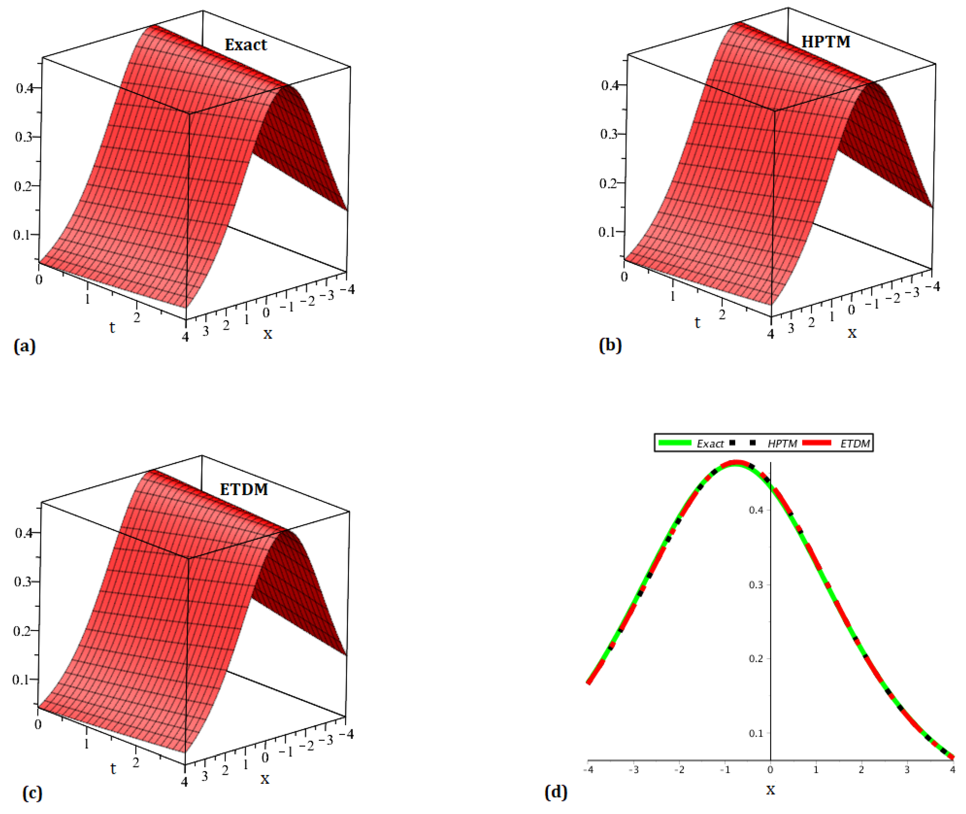
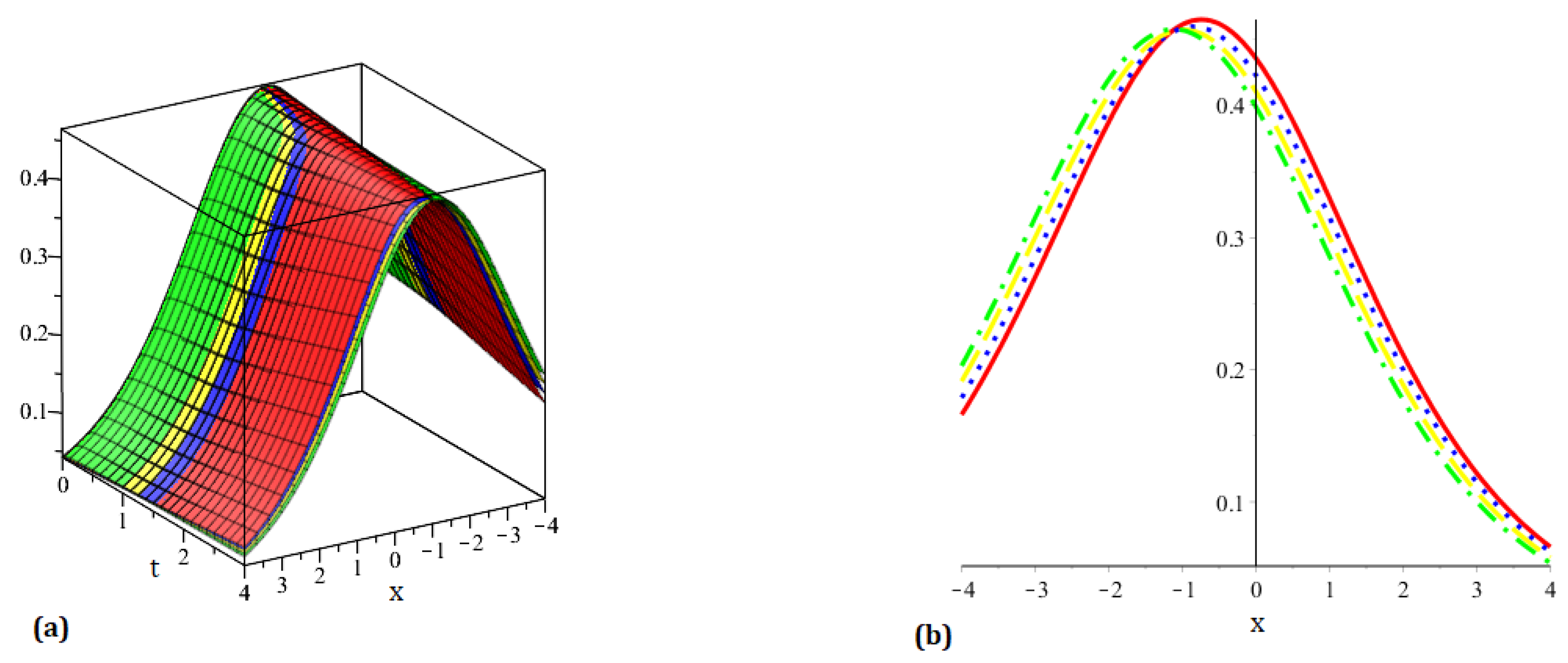
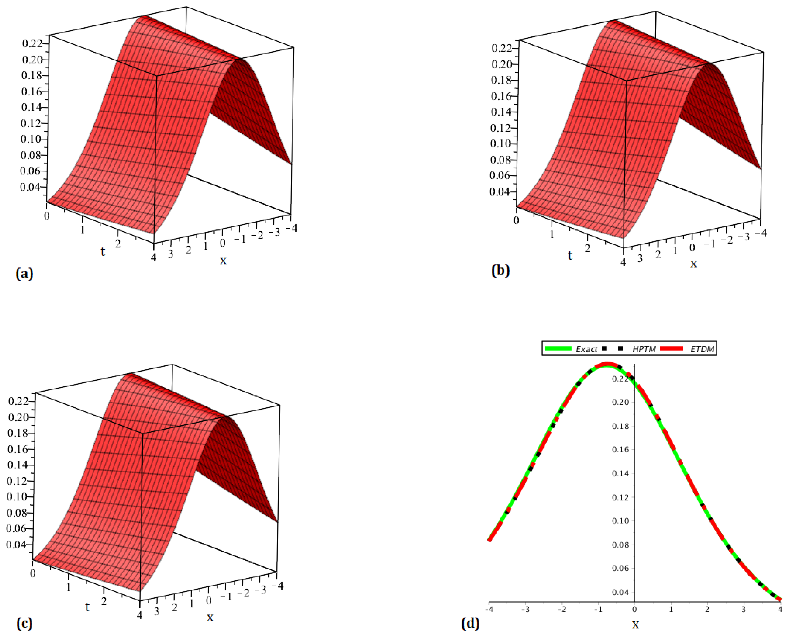
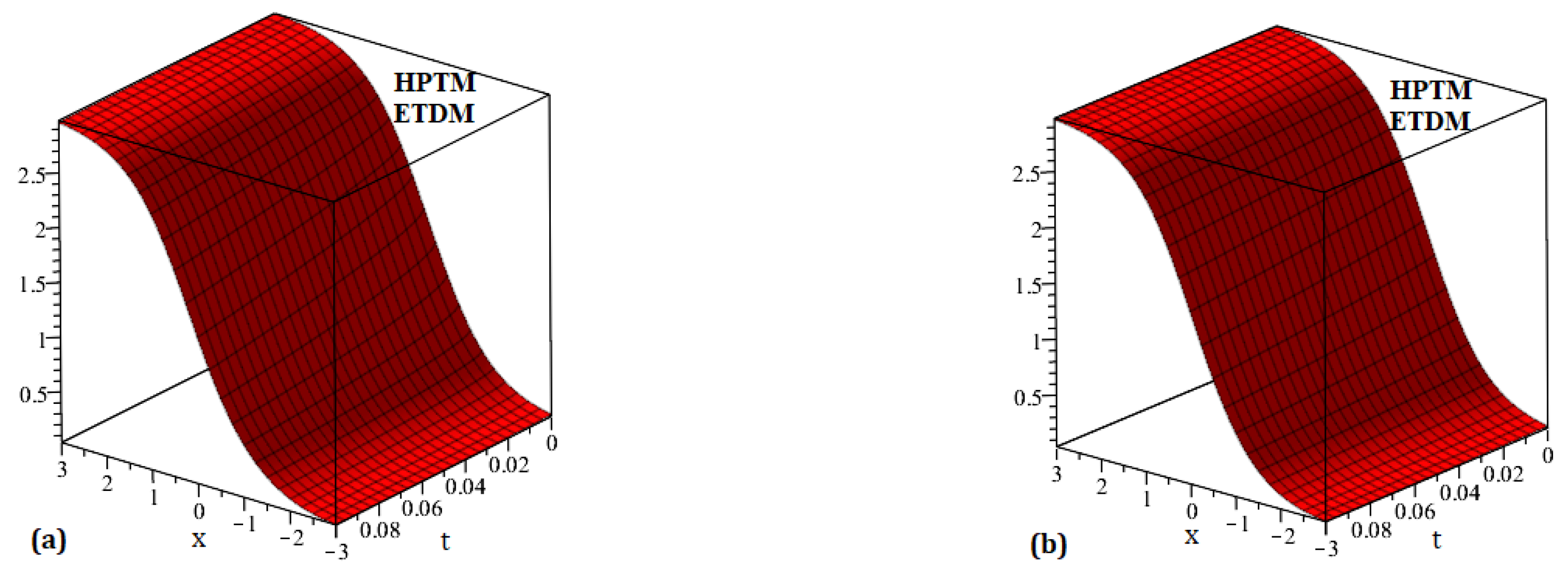
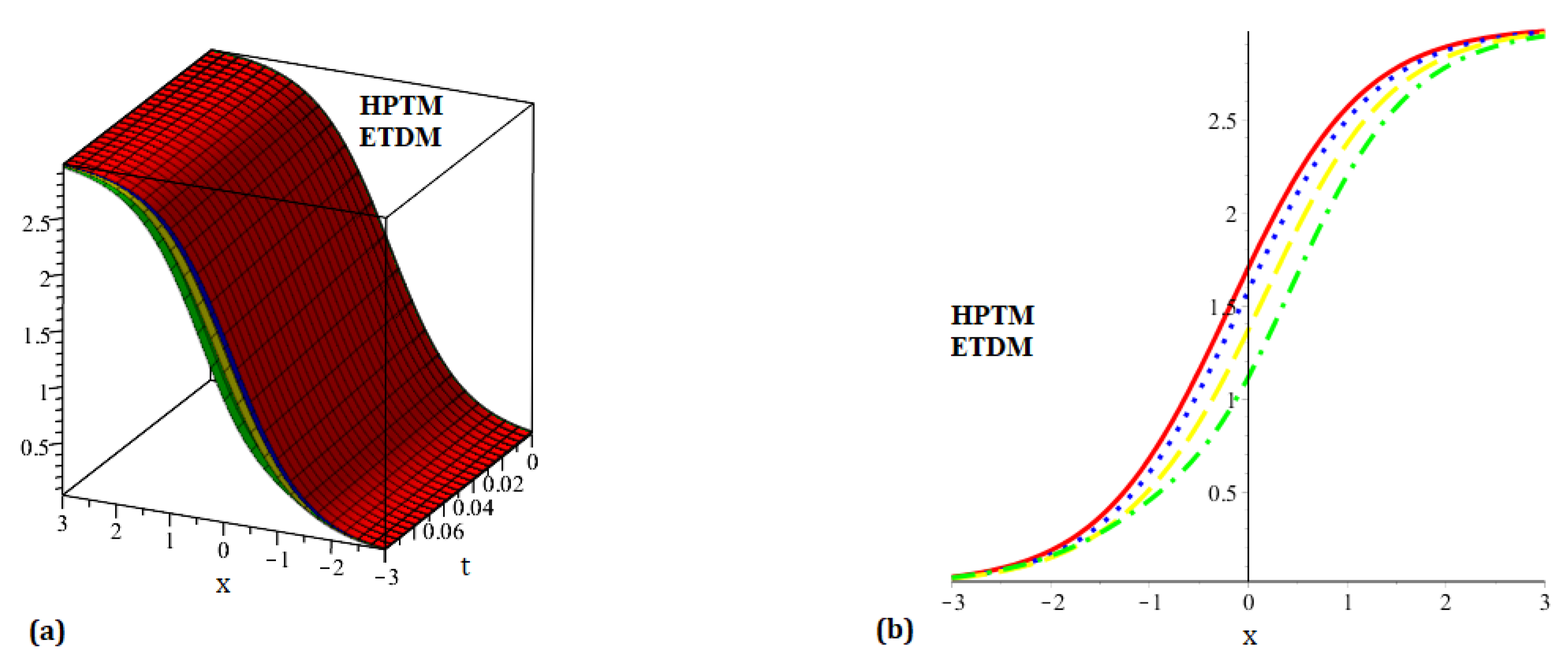
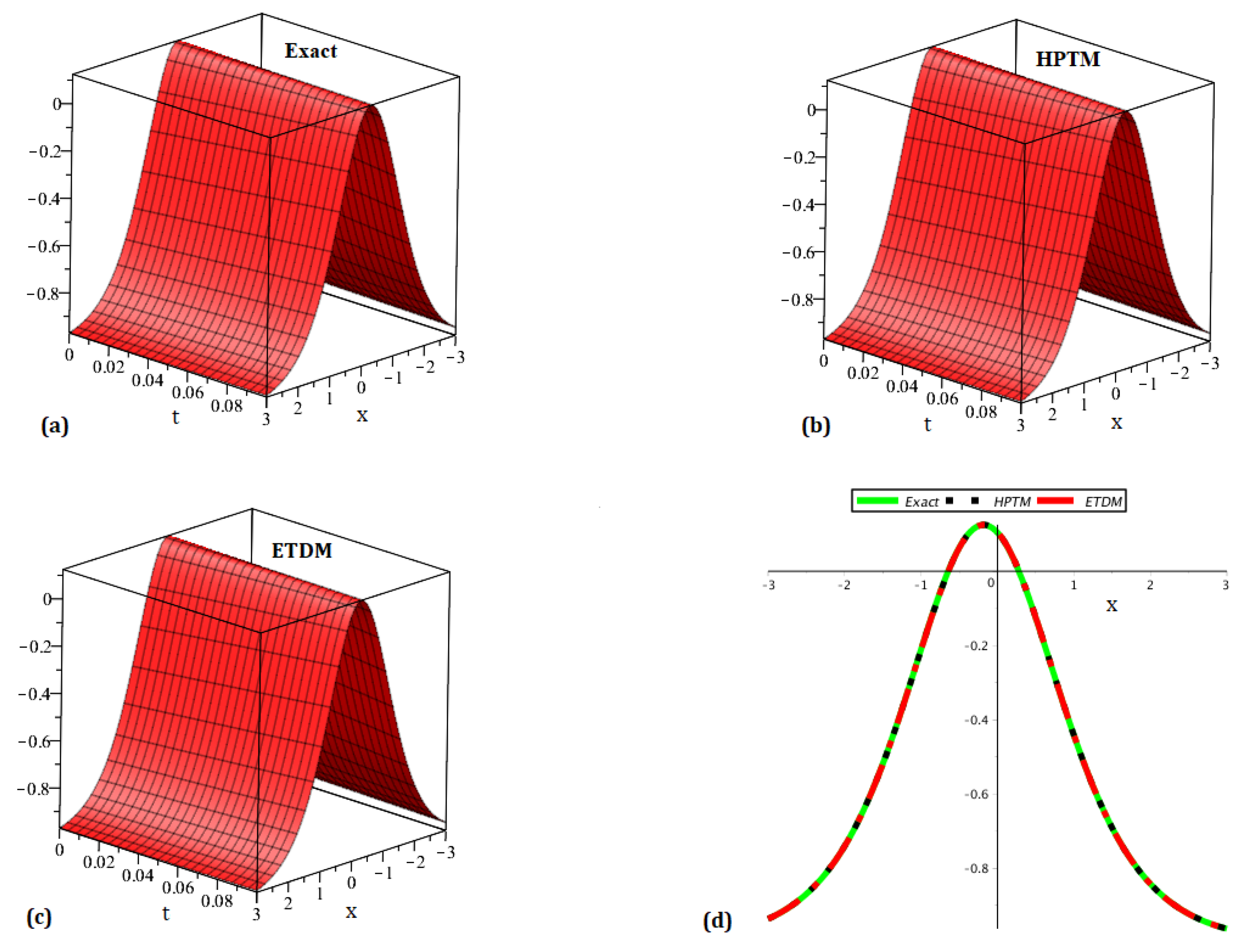
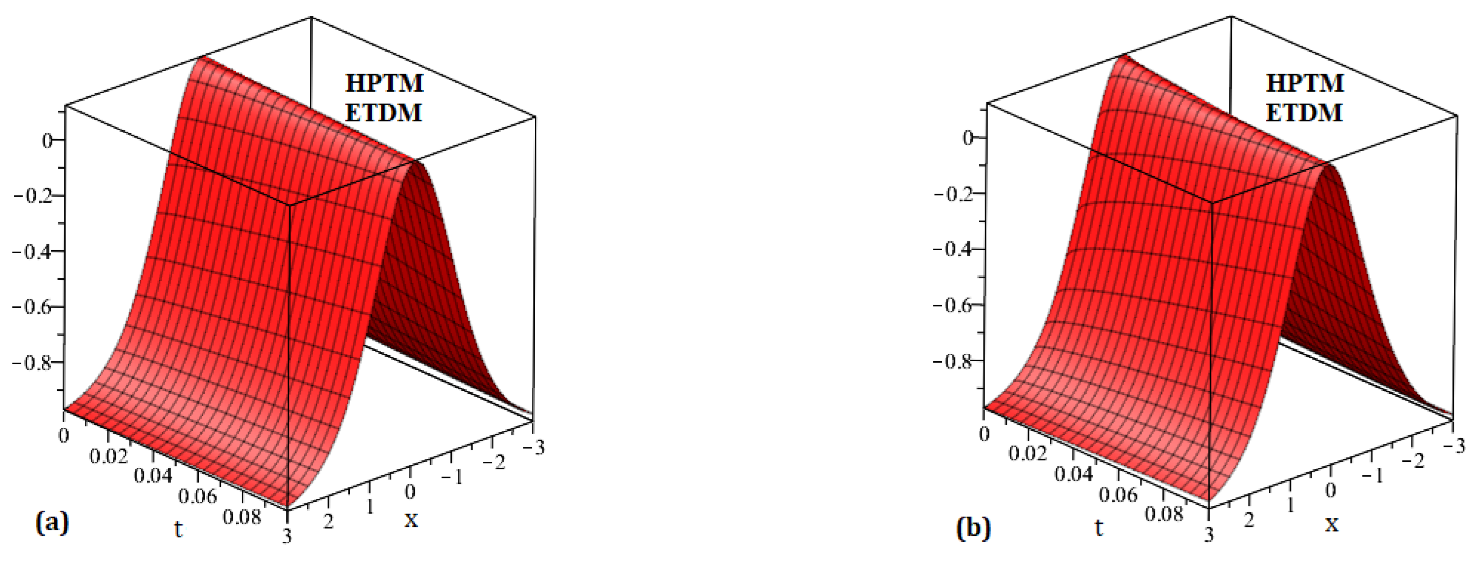
Four diagrams are shown in Figure 1: (a) the precise solution of $\mathrm{f}(\mathrm{x},\mathrm{t})$, (b) representing the HPTM solution of $\mathrm{f}(\mathrm{x},\mathrm{t})$, (c) representing the ETDM solution of $\mathrm{f}(\mathrm{x},\mathrm{t})$, and (d) representing the 2D comparison of the precise and proposed schemes solution for $\mathrm{g}(\mathrm{x},\mathrm{t})$. The graphical results demonstrate how closely the exact solution and the analytical solution match up. Figure 2 is split into two sections: the solutions for the suggested strategies are given in (a) at $\delta =0.6$ and (b) at $\delta =0.8$. Similarly, Figure 3 presents two diagrams: (a) the 3D surface solution of the suggested methods and (b) the 2D surface solution of the suggested methods of $\mathrm{f}(\mathrm{x},\mathrm{t})$. In a similar way, four diagrams are shown in Figure 4: (a) the precise solution of $\mathrm{f}(\mathrm{x},\mathrm{t})$, (b) representing the HPTM solution of $\mathrm{f}(\mathrm{x},\mathrm{t})$, (c) representing the ETDM solution of $\mathrm{f}(\mathrm{x},\mathrm{t})$, and (d) representing the 2D comparison of the precise and proposed schemes solution for $\mathrm{g}(\mathrm{x},\mathrm{t})$. Figure 5 is split into two sections: the solutions for the suggested strategies are given in (a) at $\delta =0.6$ and (b) at $\delta =0.8$. Similarly, Figure 6 presents two diagrams: (a) the 3D surface solution of the suggested methods and (b) the 2D surface solution of the suggested methods of $\mathrm{g}(\mathrm{x},\mathrm{t})$. The precise results and approximate results achieved by the proposed strategies for $\delta =0.85,0.90,0.95$ and $\delta =1$ are compared in Table 1 and Table 2. The absolute error analysis between the suggested techniques and other methods is presented in Table 3 and Table 4, demonstrating the superior accuracy of the proposed strategies over the other methods.

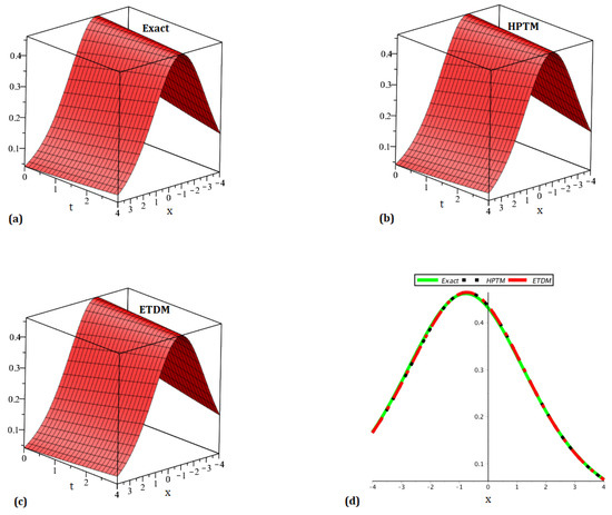
Figure 1. Plot (a) representing the precise solution, (b) HPTM solution, (c) ETDM solution, and (d) representing the comparison of the precise and proposed schemes solution for $\mathrm{f}(\mathrm{x},\mathrm{t})$.

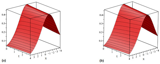
Figure 2. Plot (a) representing our approaches solution at $\delta =0.6$, (b) representing our approaches solution at $\delta =0.8$ for $\mathrm{f}(\mathrm{x},\mathrm{t})$.

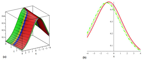
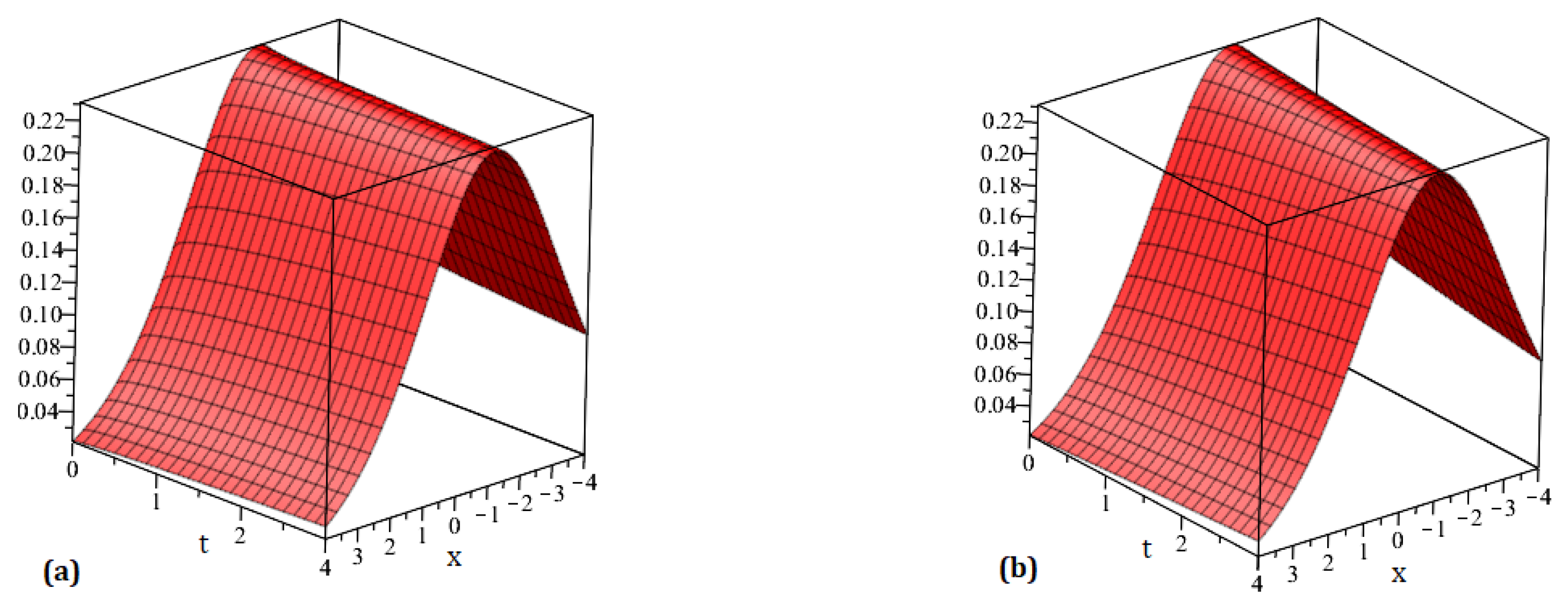
Figure 3. Plot (a) representing 3D behavior of our approaches solution (b) representing 2D behavior of our approaches solution at different orders of $\delta =0.4,0.6,0.8,1$ for $\mathrm{f}(\mathrm{x},\mathrm{t})$.

Figure 4. Plot (a) representing the precise solution, (b) HPTM solution, (c) ETDM solution, and (d) representing the comparison of the precise and proposed schemes solution for $\mathrm{g}(\mathrm{x},\mathrm{t})$.

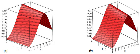
Figure 5. Plot (a) representing our approaches solution at $\delta =0.6$, (b) representing our approaches solution at $\delta =0.8$ for $\mathrm{g}(\mathrm{x},\mathrm{t})$.

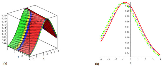
Figure 6. Plot (a) representing 3D behavior of our approaches solution (b) representing 2D behavior of our approaches solution at different orders of $\delta =0.4,0.6,0.8,1$ for $\mathrm{g}(\mathrm{x},\mathrm{t})$.

Table 1. Numerical representation of the precise and our approaches solution for $\mathrm{f}(\mathrm{x},\mathrm{t})$.

$\mathbf{t}$	$\mathbf{x}$	$\mathit{\delta }=0.85$	$\mathit{\delta }=0.90$	$\mathit{\delta }=0.95$	$\mathit{\delta }=1$ (Appro)	$\mathit{\delta }=1$ (Exact)	$\mathit{\delta }=1$ (Error)
	0.0	0.1967317176	0.1967054903	0.1966848785	0.1966687124	0.1966687124	0.0000000000000
	0.2	0.1874935332	0.1874664560	0.1874451775	0.1874284891	0.1874284890	1.000000000 $\times {10}^{-10}$
0.01	0.4	0.1780204208	0.1779928319	0.1779711521	0.1779541496	0.1779541496	0.0000000000000
	0.6	0.1684252406	0.1683974529	0.1683756179	0.1683584941	0.1683584941	0.0000000000000
	0.8	0.1588113800	0.1587836770	0.1587619095	0.1587448390	0.1587448390	0.0000000000000
	1	0.1492713947	0.1492440275	0.1492225242	0.1492056616	0.1492056615	1.000000000 $\times {10}^{-10}$
	0.0	0.1969165494	0.1968633087	0.1968190098	0.1967822290	0.1967822293	1.000000000 $\times {10}^{-10}$
	0.2	0.1876843872	0.1876294025	0.1875836580	0.1875456805	0.1875456805	0.0000000000000
0.03	0.4	0.1782149127	0.1781588717	0.1781122532	0.1780735534	0.1780735534	0.0000000000000
	0.6	0.1686211600	0.1685647004	0.1685177379	0.1684787553	0.1684787553	0.0000000000000
	0.8	0.1590067250	0.1589504244	0.1589035980	0.1588647309	0.1588647308	1.000000000 $\times {10}^{-10}$
	1	0.1494643939	0.1494087637	0.1493624982	0.1493240987	0.1493240987	0.0000000000000
	0.0	0.1970819829	0.1970098889	0.1969482590	0.1968956906	0.1968956906	0.0000000000000
	0.2	0.1878552650	0.1877807852	0.1877171266	0.1876628354	0.1876628354	0.0000000000000
0.05	0.4	0.1783890954	0.1783131634	0.1782482731	0.1781929383	0.1781929382	1.000000000 $\times {10}^{-10}$
	0.6	0.1687966638	0.1687201455	0.1686547628	0.1685990137	0.1685990137	0.0000000000000
	0.8	0.1591817521	0.1591054325	0.1590402270	0.1589846343	0.1589846343	0.0000000000000
	1	0.1496373527	0.1495619268	0.1494974915	0.1494425606	0.1494425602	0.0000000000000

Table 2. Numerical representation of the precise and our approaches solution for $\mathrm{g}(\mathrm{x},\mathrm{t})$.

$\mathbf{t}$	$\mathbf{x}$	$\mathit{\delta }=0.85$	$\mathit{\delta }=0.90$	$\mathit{\delta }=0.95$	$\mathit{\delta }=1$ (Appro)	$\mathit{\delta }=1$ (Exact)	$\mathit{\delta }=1$ (Error)
	0.0	0.0983658588	0.0983527451	0.0983424392	0.0983343562	0.0983343562	3.890000000 $\times {10}^{-12}$
	0.2	0.0937467665	0.0937332279	0.0937225887	0.0937142445	0.0937142445	1.650000000 $\times {10}^{-12}$
0.01	0.4	0.0890102104	0.0889964159	0.0889855760	0.0889770748	0.0889770748	3.830000000 $\times {10}^{-12}$
	0.6	0.0842126203	0.0841987264	0.0841878089	0.0841792470	0.0841792470	1.840000000 $\times {10}^{-12}$
	0.8	0.0794056900	0.0793918385	0.0793809547	0.0793724195	0.0793724195	2.450000000 $\times {10}^{-12}$
	1	0.0746356973	0.0746220137	0.0746112621	0.0746028307	0.0746028307	1.040000000 $\times {10}^{-12}$
	0.0	0.0984582746	0.0984316543	0.0984095049	0.0983911146	0.0983911146	2.800000000 $\times {10}^{-12}$
	0.2	0.0938421935	0.0938147012	0.0937918289	0.0937728402	0.0937728402	1.016000000 $\times {10}^{-11}$
0.03	0.4	0.0891074563	0.0890794358	0.0890561266	0.0890367767	0.0890367767	6.580000000 $\times {10}^{-12}$
	0.6	0.0843105799	0.0842823502	0.0842588689	0.0842393776	0.0842393776	2.180000000 $\times {10}^{-12}$
	0.8	0.0795033624	0.0794752122	0.0794517990	0.0794323654	0.0794323654	7.860000000 $\times {10}^{-12}$
	1	0.0747321969	0.0747043818	0.0746812490	0.0746620493	0.0746620493	3.220000000 $\times {10}^{-12}$
	0.0	0.0985409915	0.0985049444	0.0984741294	0.0984478452	0.0984478452	2.600000000 $\times {10}^{-12}$
	0.2	0.0939276325	0.0938903926	0.0938585632	0.0938314176	0.0938314176	3.100000000 $\times {10}^{-12}$
0.05	0.4	0.0891945477	0.0891565817	0.0891241365	0.0890964691	0.0890964691	7.900000000 $\times {10}^{-12}$
	0.6	0.0843983319	0.0843600727	0.0843273813	0.0842995068	0.0842995068	1.600000000 $\times {10}^{-12}$
	0.8	0.0795908760	0.0795527162	0.0795201134	0.0794923171	0.0794923171	6.600000000 $\times {10}^{-12}$
	1	0.0748186763	0.0747809633	0.0747487457	0.0747212800	0.0747212800	5.300000000 $\times {10}^{-12}$

Table 3. Comparative analysis among our approaches solution homotopy decomposition method (HDM), the natural decomposition method (NDM), and the modified Mittag-Leffler function method (MMLFM) for $\mathrm{f}(\mathrm{x},\mathrm{t})$.

$\mathbf{x}$	$\mathbf{t}$	Error NDM	Error HDM	Error MGMFM	Error of Proposed Methods
−10	0.1	2.95039 $\times {10}^{-8}$	2.99039 $\times {10}^{-8}$	5.0551 $\times {10}^{-10}$	0.0000000000
	0.2	2.30335 $\times {10}^{-7}$	2.33335 $\times {10}^{-7}$	1.76949 $\times {10}^{-9}$	2.00000 $\times {10}^{-11}$
−5	0.1	3.93592 $\times {10}^{-6}$	3.96592 $\times {10}^{-6}$	1.05846 $\times {10}^{-6}$	0.0000000000
	0.2	0.0000308049	0.0000338049	0.000037098	2.00000 $\times {10}^{-10}$
5	0.1	0.000202966	0.00000397592	0.0000138323	0.0000000000
	0.2	0.000515586	0.0000378049	0.0000633656	2.00000 $\times {10}^{-11}$
10	0.1	2.11254 $\times {10}^{-8}$	2.96039 $\times {10}^{-8}$	6.59404 $\times {10}^{-10}$	1.00000 $\times {10}^{-12}$
	0.2	2.28173 $\times {10}^{-7}$	2.37335 $\times {10}^{-7}$	3.01639 $\times {10}^{-9}$	3.00000 $\times {10}^{-12}$

Table 4. Comparative analysis among our approaches solution with NDM, HDM, and MGMFM for $\mathrm{g}(\mathrm{x},\mathrm{t})$.

$\mathbf{x}$	$\mathbf{t}$	Error NDM	Error HDM	Error MGMFM	Error of Proposed Methods
−10	0.1	2.08624 $\times {10}^{-8}$	2.18624 $\times {10}^{-8}$	3.57125 $\times {10}^{-10}$	5.00000 $\times {10}^{-14}$
	0.2	1.62872 $\times {10}^{-7}$	1.64872 $\times {10}^{-7}$	1.25122 $\times {10}^{-9}$	8.30000 $\times {10}^{-12}$
−5	0.1	2.78312 $\times {10}^{-6}$	2.88312 $\times {10}^{-6}$	7.48447 $\times {10}^{-6}$	7.50000 $\times {10}^{-12}$
	0.2	0.0000217824	0.0000287824	0.0000262322	6.78000 $\times {10}^{-11}$
5	0.1	2.9094 $\times {10}^{-6}$	2.98312 $\times {10}^{-6}$	9.78092 $\times {10}^{-6}$	1.03000 $\times {10}^{-12}$
	0.2	0.0000238036	0.0000247824	0.000044806	7.70000 $\times {10}^{-12}$
10	0.1	2.19313 $\times {10}^{-8}$	2.09624 $\times {10}^{-8}$	4.6629 $\times {10}^{-10}$	3.47000 $\times {10}^{-13}$
	0.2	1.79991 $\times {10}^{-7}$	1.72872 $\times {10}^{-7}$	2.13291 $\times {10}^{-9}$	1.51000 $\times {10}^{-12}$

7.2. Example

Assuming the nonlinear fractional dispersive long wave system of the form

$$\begin{array}{cc}\hfill & {\displaystyle \frac{{\partial }^{\delta }\mathrm{f}}{\partial {\mathrm{t}}^{\delta }}}=-{\mathrm{g}}_{\mathrm{x}}(\mathrm{x},\mathrm{t})-{\displaystyle \frac{1}{2}}{\left({\mathrm{f}}^2(\mathrm{x},\mathrm{t})\right)}_{\mathrm{x}},\hfill \\ \hfill & {\displaystyle \frac{{\partial }^{\delta }\mathrm{g}}{\partial {\mathrm{t}}^{\delta }}}=-{\left(\mathrm{f}(\mathrm{x},\mathrm{t})+{\mathrm{f}}_{\mathrm{x}\mathrm{x}}(\mathrm{x},\mathrm{t})+\mathrm{f}(\mathrm{x},\mathrm{t})\mathrm{g}(\mathrm{x},\mathrm{t})\right)}_{\mathrm{x}},\hfill \end{array}$$

(56)

with

$$\mathrm{f}(\mathrm{x},0)=\kappa \left[tanh\left({\displaystyle \frac{\mathbf{b}}{2}}+{\displaystyle \frac{\kappa \mathrm{x}}{2}}\right)+1\right],\mathrm{g}(\mathrm{x},0)=-1+{\displaystyle \frac{1}{2}}{\kappa }^2{sech}^2\left({\displaystyle \frac{\mathbf{b}}{2}}+{\displaystyle \frac{\kappa \mathrm{x}}{2}}\right).$$

Case I: Application of HPTM

Executing the ET, we have

$$\begin{array}{cc}\hfill & \mathtt{E}\left[{\displaystyle \frac{{\partial }^{\delta }\mathrm{f}}{\partial {\mathrm{t}}^{\delta }}}\right]=\mathtt{E}\left[-{\mathrm{g}}_{\mathrm{x}}(\mathrm{x},\mathrm{t})-{\displaystyle \frac{1}{2}}{\left({\mathrm{f}}^2(\mathrm{x},\mathrm{t})\right)}_{\mathrm{x}}\right],\hfill \\ \hfill & \mathtt{E}\left[{\displaystyle \frac{{\partial }^{\delta }\mathrm{g}}{\partial {\mathrm{t}}^{\delta }}}\right]=\mathtt{E}\left[-{\left(\mathrm{f}(\mathrm{x},\mathrm{t})+{\mathrm{f}}_{\mathrm{x}\mathrm{x}}(\mathrm{x},\mathrm{t})+\mathrm{f}(\mathrm{x},\mathrm{t})\mathrm{g}(\mathrm{x},\mathrm{t})\right)}_{\mathrm{x}}\right].\hfill \end{array}$$

(57)

Thus we obtain

$$\begin{array}{cc}\hfill & {\displaystyle \frac{1}{u^{\delta }}}\{M\left(u\right)-u^2\mathrm{f}\left(0\right)\}=\mathtt{E}\left[-{\mathrm{g}}_{\mathrm{x}}(\mathrm{x},\mathrm{t})-{\displaystyle \frac{1}{2}}{\left({\mathrm{f}}^2(\mathrm{x},\mathrm{t})\right)}_{\mathrm{x}}\right],\hfill \\ \hfill & {\displaystyle \frac{1}{u^{\delta }}}\{M\left(u\right)-u^2\mathrm{g}\left(0\right)\}=\mathtt{E}\left[-{\left(\mathrm{f}(\mathrm{x},\mathrm{t})+{\mathrm{f}}_{\mathrm{x}\mathrm{x}}(\mathrm{x},\mathrm{t})+\mathrm{f}(\mathrm{x},\mathrm{t})\mathrm{g}(\mathrm{x},\mathrm{t})\right)}_{\mathrm{x}}\right],\hfill \end{array}$$

(58)

$$\begin{array}{cc}\hfill & M\left(u\right)=u^2\mathrm{f}\left(0\right)+u^{\delta }\left[-{\mathrm{g}}_{\mathrm{x}}(\mathrm{x},\mathrm{t})-{\displaystyle \frac{1}{2}}{\left({\mathrm{f}}^2(\mathrm{x},\mathrm{t})\right)}_{\mathrm{x}}\right],\hfill \\ \hfill & M\left(u\right)=u^2\mathrm{g}\left(0\right)+u^{\delta }\left[-{\left(\mathrm{f}(\mathrm{x},\mathrm{t})+{\mathrm{f}}_{\mathrm{x}\mathrm{x}}(\mathrm{x},\mathrm{t})+\mathrm{f}(\mathrm{x},\mathrm{t})\mathrm{g}(\mathrm{x},\mathrm{t})\right)}_{\mathrm{x}}\right].\hfill \end{array}$$

(59)

Executing the inverse ET, we have

$$\begin{array}{cc}\hfill & \mathrm{f}(\mathrm{x},\mathrm{t})=\mathrm{f}\left(0\right)+{\mathtt{E}}^{-1}\left[u^{\delta }\left\{\mathtt{E}\left(-{\mathrm{g}}_{\mathrm{x}}(\mathrm{x},\mathrm{t})-{\displaystyle \frac{1}{2}}{\left({\mathrm{f}}^2(\mathrm{x},\mathrm{t})\right)}_{\mathrm{x}}\right)\right\}\right],\hfill \\ \hfill & \mathrm{g}(\mathrm{x},\mathrm{t})=\mathrm{g}\left(0\right)+{\mathtt{E}}^{-1}\left[u^{\delta }\left\{\mathtt{E}\left(-{\left(\mathrm{f}(\mathrm{x},\mathrm{t})+{\mathrm{f}}_{\mathrm{x}\mathrm{x}}(\mathrm{x},\mathrm{t})+\mathrm{f}(\mathrm{x},\mathrm{t})\mathrm{g}(\mathrm{x},\mathrm{t})\right)}_{\mathrm{x}}\right)\right\}\right],\hfill \\ \hfill & \mathrm{f}(\mathrm{x},\mathrm{t})=\kappa \left[tanh\left({\displaystyle \frac{\mathbf{b}}{2}}+{\displaystyle \frac{\kappa \mathrm{x}}{2}}\right)+1\right]+{\mathtt{E}}^{-1}\left[u^{\delta }\left\{\mathtt{E}\left(-{\mathrm{g}}_{\mathrm{x}}(\mathrm{x},\mathrm{t})-{\displaystyle \frac{1}{2}}{\left({\mathrm{f}}^2(\mathrm{x},\mathrm{t})\right)}_{\mathrm{x}}\right)\right\}\right],\hfill \\ \hfill & \mathrm{g}(\mathrm{x},\mathrm{t})=-1+{\displaystyle \frac{1}{2}}{\kappa }^2{sech}^2\left({\displaystyle \frac{\mathbf{b}}{2}}+{\displaystyle \frac{\kappa \mathrm{x}}{2}}\right)+{\mathtt{E}}^{-1}\left[u^{\delta }\left\{\mathtt{E}\left(-{\left(\mathrm{f}(\mathrm{x},\mathrm{t})+{\mathrm{f}}_{\mathrm{x}\mathrm{x}}(\mathrm{x},\mathrm{t})+\mathrm{f}(\mathrm{x},\mathrm{t})\mathrm{g}(\mathrm{x},\mathrm{t})\right)}_{\mathrm{x}}\right)\right\}\right].\hfill \end{array}$$

(60)

In the context of the homotopy perturbation method, we have

$$\begin{array}{cc}\hfill & \sum _{k=0}^{\infty }{ϵ}^k{\mathrm{f}}_k(\mathrm{x},\mathrm{t})=\kappa \left[tanh\left({\displaystyle \frac{\mathbf{b}}{2}}+{\displaystyle \frac{\kappa \mathrm{x}}{2}}\right)+1\right]+ϵ\left({\mathtt{E}}^{-1}\left[u^{\delta }\mathtt{E}\left[-\left(\sum _{k=0}^{\infty }{ϵ}^k{\mathrm{g}}_k(\mathrm{x},\mathrm{t})\right)-{\displaystyle \frac{1}{2}}{\left(\sum _{k=0}^{\infty }{ϵ}^k{H}_k(\mathrm{x},\mathrm{t})\right)}_{\mathrm{x}}\right]\right]\right),\hfill \\ \hfill & \sum _{k=0}^{\infty }{ϵ}^k{\mathrm{g}}_k(\mathrm{x},\mathrm{t})=-1+{\displaystyle \frac{1}{2}}{\kappa }^2{sech}^2\left({\displaystyle \frac{\mathbf{b}}{2}}+{\displaystyle \frac{\kappa \mathrm{x}}{2}}\right)+ϵ\left({\mathtt{E}}^{-1}\right[u^{\delta }\mathtt{E}[-(\left(\sum _{k=0}^{\infty }{ϵ}^k{\mathrm{f}}_k(\mathrm{x},\mathrm{t})\right)+{\left(\sum _{k=0}^{\infty }{ϵ}^k{\mathrm{f}}_k(\mathrm{x},\mathrm{t})\right)}_{\mathrm{x}\mathrm{x}}\hfill \\ \hfill & +\left(\sum _{k=0}^{\infty }{ϵ}^k{H}_k(\mathrm{x},\mathrm{t})\right){)}_{\mathrm{x}}\left]\right]).\hfill \end{array}$$

(61)

Equating the similar components of $ϵ$, we obtain

$$\begin{array}{cc}\hfill & {ϵ}^0:{\mathrm{f}}_0(\mathrm{x},\mathrm{t})=\kappa \left[tanh\left({\displaystyle \frac{\mathbf{b}}{2}}+{\displaystyle \frac{\kappa \mathrm{x}}{2}}\right)+1\right],\hfill \\ \hfill & {ϵ}^0:{\mathrm{g}}_0(\mathrm{x},\mathrm{t})=-1+{\displaystyle \frac{1}{2}}{\kappa }^2{sech}^2\left({\displaystyle \frac{\mathbf{b}}{2}}+{\displaystyle \frac{\kappa \mathrm{x}}{2}}\right),\hfill \\ \hfill & {ϵ}^1:{\mathrm{f}}_1(\mathrm{x},\mathrm{t})=-{\displaystyle \frac{1}{2}}{\displaystyle \frac{{\kappa }^3}{{cosh}^2\left(\frac{\mathbf{b}}{2}+\frac{\kappa \mathrm{x}}{2}\right)}}{\displaystyle \frac{{\mathrm{t}}^{\delta }}{\mathsf{\Gamma }(\delta +1)}},\hfill \\ \hfill & {ϵ}^1:{\mathrm{g}}_1(\mathrm{x},\mathrm{t})={\displaystyle \frac{1}{2}}{\displaystyle \frac{{\kappa }^{4}sinh\left(\frac{\mathbf{b}}{2}+\frac{\kappa \mathrm{x}}{2}\right)}{{cosh}^3\left(\frac{\mathbf{b}}{2}+\frac{\kappa \mathrm{x}}{2}\right)}}{\displaystyle \frac{{\mathrm{t}}^{\delta }}{\mathsf{\Gamma }(\delta +1)}},\hfill \\ \hfill & {ϵ}^2:{\mathrm{f}}_2(\mathrm{x},\mathrm{t})=-{\displaystyle \frac{1}{2}}{\displaystyle \frac{{\kappa }^{5}sinh\left(\frac{\mathbf{b}}{2}+\frac{\kappa \mathrm{x}}{2}\right)}{{cosh}^3\left(\frac{\mathbf{b}}{2}+\frac{\kappa \mathrm{x}}{2}\right)}}{\displaystyle \frac{{\mathrm{t}}^{2\delta }}{\mathsf{\Gamma }(2\delta +1)}},\hfill \\ \hfill & {ϵ}^2:{\mathrm{g}}_2(\mathrm{x},\mathrm{t})={\displaystyle \frac{1}{4}}{\displaystyle \frac{{\kappa }^6\left(2{cosh}^2\left(\frac{\mathbf{b}}{2}+\frac{\kappa \mathrm{x}}{2}\right)-3\right)}{{cosh}^4\left(\frac{\mathbf{b}}{2}+\frac{\kappa \mathrm{x}}{2}\right)}}{\displaystyle \frac{{\mathrm{t}}^{2\delta }}{\mathsf{\Gamma }(2\delta +1)}},\hfill \\ \hfill & {ϵ}^3:{\mathrm{f}}_3(\mathrm{x},\mathrm{t})=-{\displaystyle \frac{1}{4}}{\displaystyle \frac{{\kappa }^7\left(2{cosh}^3\left(\frac{\mathbf{b}}{2}+\frac{\kappa \mathrm{x}}{2}\right)-3cosh\left(\frac{\mathbf{b}}{2}+\frac{\kappa \mathrm{x}}{2}\right)+2sinh\left(\frac{\mathbf{b}}{2}+\frac{\kappa \mathrm{x}}{2}\right)\right)}{{cosh}^5\left(\frac{\mathbf{b}}{2}+\frac{\kappa \mathrm{x}}{2}\right)}}{\displaystyle \frac{{\mathrm{t}}^{3\delta }}{\mathsf{\Gamma }(3\delta +1)}}+\hfill \\ \hfill & {\displaystyle \frac{1}{4}}{\displaystyle \frac{{\kappa }^{7}sinh\left(\frac{\mathbf{b}}{2}+\frac{\kappa \mathrm{x}}{2}\right)\mathsf{\Gamma }(2\delta +1)}{cosh\left(\frac{\mathbf{b}}{2}+\frac{\kappa \mathrm{x}}{2}\right)\mathsf{\Gamma }{(\delta +1)}^2}}{\displaystyle \frac{{\mathrm{t}}^{3\delta }}{\mathsf{\Gamma }(3\delta +1)}},\hfill \\ \hfill & {ϵ}^3:{\mathrm{g}}_3(\mathrm{x},\mathrm{t})={\displaystyle \frac{1}{4}}{\displaystyle \frac{{\kappa }^8\left(2sinh\left(\frac{\mathbf{b}}{2}+\frac{\kappa \mathrm{x}}{2}\right){cosh}^3\left(\frac{\mathbf{b}}{2}+\frac{\kappa \mathrm{x}}{2}\right)+4{cosh}^2\left(\frac{\mathbf{b}}{2}+\frac{\kappa \mathrm{x}}{2}\right)-6sinh\left(\frac{\mathbf{b}}{2}+\frac{\kappa \mathrm{x}}{2}\right)cosh\left(\frac{\mathbf{b}}{2}+\frac{\kappa \mathrm{x}}{2}\right)-5\right)}{{cosh}^6\left(\frac{\mathbf{b}}{2}+\frac{\kappa \mathrm{x}}{2}\right)}}\hfill \\ \hfill & {\displaystyle \frac{{\mathrm{t}}^{3\delta }}{\mathsf{\Gamma }(3\delta +1)}}-{\displaystyle \frac{1}{8}}{\displaystyle \frac{{\kappa }^8\left(4{cosh}^2\left(\frac{\mathbf{b}}{2}+\frac{\kappa \mathrm{x}}{2}\right)-5\right)\mathsf{\Gamma }(2\delta +1)}{{cosh}^6\left(\frac{\mathbf{b}}{2}+\frac{\kappa \mathrm{x}}{2}\right)\mathsf{\Gamma }{(\delta +1)}^2}}{\displaystyle \frac{{\mathrm{t}}^{3\delta }}{\mathsf{\Gamma }(3\delta +1)}},\hfill \\ \hfill & ⋮\hfill \end{array}$$

Thus, the approximate solution is computed as

$$\begin{array}{cc}\hfill & \mathrm{f}(\mathrm{x},\mathrm{t})={\mathrm{f}}_0(\mathrm{x},\mathrm{t})+{\mathrm{f}}_1(\mathrm{x},\mathrm{t})+{\mathrm{f}}_2(\mathrm{x},\mathrm{t})+{\mathrm{f}}_3(\mathrm{x},\mathrm{t})+\cdots \hfill \\ \hfill & \mathrm{f}(\mathrm{x},\mathrm{t})=\kappa \left[tanh\left({\displaystyle \frac{\mathbf{b}}{2}}+{\displaystyle \frac{\kappa \mathrm{x}}{2}}\right)+1\right]-{\displaystyle \frac{1}{2}}{\displaystyle \frac{{\kappa }^3}{{cosh}^2\left(\frac{\mathbf{b}}{2}+\frac{\kappa \mathrm{x}}{2}\right)}}{\displaystyle \frac{{\mathrm{t}}^{\delta }}{\mathsf{\Gamma }(\delta +1)}}-{\displaystyle \frac{1}{2}}{\displaystyle \frac{{\kappa }^{5}sinh\left(\frac{\mathbf{b}}{2}+\frac{\kappa \mathrm{x}}{2}\right)}{{cosh}^3\left(\frac{\mathbf{b}}{2}+\frac{\kappa \mathrm{x}}{2}\right)}}{\displaystyle \frac{{\mathrm{t}}^{2\delta }}{\mathsf{\Gamma }(2\delta +1)}}\hfill \\ \hfill & -{\displaystyle \frac{1}{4}}{\displaystyle \frac{{\kappa }^7\left(2{cosh}^3\left(\frac{\mathbf{b}}{2}+\frac{\kappa \mathrm{x}}{2}\right)-3cosh\left(\frac{\mathbf{b}}{2}+\frac{\kappa \mathrm{x}}{2}\right)+2sinh\left(\frac{\mathbf{b}}{2}+\frac{\kappa \mathrm{x}}{2}\right)\right)}{{cosh}^5\left(\frac{\mathbf{b}}{2}+\frac{\kappa \mathrm{x}}{2}\right)}}{\displaystyle \frac{{\mathrm{t}}^{3\delta }}{\mathsf{\Gamma }(3\delta +1)}}+\hfill \\ \hfill & {\displaystyle \frac{1}{4}}{\displaystyle \frac{{\kappa }^{7}sinh\left(\frac{\mathbf{b}}{2}+\frac{\kappa \mathrm{x}}{2}\right)\mathsf{\Gamma }(2\delta +1)}{cosh\left(\frac{\mathbf{b}}{2}+\frac{\kappa \mathrm{x}}{2}\right)\mathsf{\Gamma }{(\delta +1)}^2}}{\displaystyle \frac{{\mathrm{t}}^{3\delta }}{\mathsf{\Gamma }(3\delta +1)}}+\cdots \hfill \\ \hfill & \mathrm{g}(\mathrm{x},\mathrm{t})={\mathrm{g}}_0(\mathrm{x},\mathrm{t})+{\mathrm{g}}_1(\mathrm{x},\mathrm{t})+{\mathrm{g}}_2(\mathrm{x},\mathrm{t})+{\mathrm{g}}_3(\mathrm{x},\mathrm{t})+\cdots \hfill \\ \hfill & \mathrm{g}(\mathrm{x},\mathrm{t})=-1+{\displaystyle \frac{1}{2}}{\kappa }^2{sech}^2\left({\displaystyle \frac{\mathbf{b}}{2}}+{\displaystyle \frac{\kappa \mathrm{x}}{2}}\right)+{\displaystyle \frac{1}{2}}{\displaystyle \frac{{\kappa }^{4}sinh\left(\frac{\mathbf{b}}{2}+\frac{\kappa \mathrm{x}}{2}\right)}{{cosh}^3\left(\frac{\mathbf{b}}{2}+\frac{\kappa \mathrm{x}}{2}\right)}}{\displaystyle \frac{{\mathrm{t}}^{\delta }}{\mathsf{\Gamma }(\delta +1)}}+{\displaystyle \frac{1}{4}}{\displaystyle \frac{{\kappa }^6\left(2{cosh}^2\left(\frac{\mathbf{b}}{2}+\frac{\kappa \mathrm{x}}{2}\right)-3\right)}{{cosh}^4\left(\frac{\mathbf{b}}{2}+\frac{\kappa \mathrm{x}}{2}\right)}}{\displaystyle \frac{{\mathrm{t}}^{2\delta }}{\mathsf{\Gamma }(2\delta +1)}}+\hfill \\ \hfill & {\displaystyle \frac{1}{4}}{\displaystyle \frac{{\kappa }^8\left(2sinh\left(\frac{\mathbf{b}}{2}+\frac{\kappa \mathrm{x}}{2}\right){cosh}^3\left(\frac{\mathbf{b}}{2}+\frac{\kappa \mathrm{x}}{2}\right)+4{cosh}^2\left(\frac{\mathbf{b}}{2}+\frac{\kappa \mathrm{x}}{2}\right)-6sinh\left(\frac{\mathbf{b}}{2}+\frac{\kappa \mathrm{x}}{2}\right)cosh\left(\frac{\mathbf{b}}{2}+\frac{\kappa \mathrm{x}}{2}\right)-5\right)}{{cosh}^6\left(\frac{\mathbf{b}}{2}+\frac{\kappa \mathrm{x}}{2}\right)}}\hfill \\ \hfill & {\displaystyle \frac{{\mathrm{t}}^{3\delta }}{\mathsf{\Gamma }(3\delta +1)}}-{\displaystyle \frac{1}{8}}{\displaystyle \frac{{\kappa }^8\left(4{cosh}^2\left(\frac{\mathbf{b}}{2}+\frac{\kappa \mathrm{x}}{2}\right)-5\right)\mathsf{\Gamma }(2\delta +1)}{{cosh}^6\left(\frac{\mathbf{b}}{2}+\frac{\kappa \mathrm{x}}{2}\right)\mathsf{\Gamma }{(\delta +1)}^2}}{\displaystyle \frac{{\mathrm{t}}^{3\delta }}{\mathsf{\Gamma }(3\delta +1)}}+\cdots \hfill \end{array}$$

Case II: Application of ETDM

Executing the ET, we have

$$\begin{array}{cc}\hfill & \mathtt{E}\left[{\displaystyle \frac{{\partial }^{\delta }\mathrm{f}}{\partial {\mathrm{t}}^{\delta }}}\right]=\mathtt{E}\left[-{\mathrm{g}}_{\mathrm{x}}(\mathrm{x},\mathrm{t})-{\displaystyle \frac{1}{2}}{\left({\mathrm{f}}^2(\mathrm{x},\mathrm{t})\right)}_{\mathrm{x}}\right],\hfill \\ \hfill & \mathtt{E}\left[{\displaystyle \frac{{\partial }^{\delta }\mathrm{g}}{\partial {\mathrm{t}}^{\delta }}}\right]=\mathtt{E}\left[-{\left(\mathrm{f}(\mathrm{x},\mathrm{t})+{\mathrm{f}}_{\mathrm{x}\mathrm{x}}(\mathrm{x},\mathrm{t})+\mathrm{f}(\mathrm{x},\mathrm{t})\mathrm{g}(\mathrm{x},\mathrm{t})\right)}_{\mathrm{x}}\right].\hfill \end{array}$$

(62)

Thus we obtain

$$\begin{array}{cc}\hfill & {\displaystyle \frac{1}{u^{\delta }}}\{M\left(u\right)-u^2\mathrm{f}\left(0\right)\}=\mathtt{E}\left[-{\mathrm{g}}_{\mathrm{x}}(\mathrm{x},\mathrm{t})-{\displaystyle \frac{1}{2}}{\left({\mathrm{f}}^2(\mathrm{x},\mathrm{t})\right)}_{\mathrm{x}}\right],\hfill \\ \hfill & {\displaystyle \frac{1}{u^{\delta }}}\{M\left(u\right)-u^2\mathrm{g}\left(0\right)\}=\mathtt{E}\left[-{\left(\mathrm{f}(\mathrm{x},\mathrm{t})+{\mathrm{f}}_{\mathrm{x}\mathrm{x}}(\mathrm{x},\mathrm{t})+\mathrm{f}(\mathrm{x},\mathrm{t})\mathrm{g}(\mathrm{x},\mathrm{t})\right)}_{\mathrm{x}}\right],\hfill \end{array}$$

(63)

$$\begin{array}{cc}\hfill & M\left(u\right)=u^2\mathrm{f}\left(0\right)+u^{\delta }\left[-{\mathrm{g}}_{\mathrm{x}}(\mathrm{x},\mathrm{t})-{\displaystyle \frac{1}{2}}{\left({\mathrm{f}}^2(\mathrm{x},\mathrm{t})\right)}_{\mathrm{x}}\right],\hfill \\ \hfill & M\left(u\right)=u^2\mathrm{g}\left(0\right)+u^{\delta }\left[-{\left(\mathrm{f}(\mathrm{x},\mathrm{t})+{\mathrm{f}}_{\mathrm{x}\mathrm{x}}(\mathrm{x},\mathrm{t})+\mathrm{f}(\mathrm{x},\mathrm{t})\mathrm{g}(\mathrm{x},\mathrm{t})\right)}_{\mathrm{x}}\right].\hfill \end{array}$$

(64)

Executing the inverse ET, we have

$$\begin{array}{cc}\hfill & \mathrm{f}(\mathrm{x},\mathrm{t})=\mathrm{f}\left(0\right)+{\mathtt{E}}^{-1}\left[u^{\delta }\left\{\mathtt{E}\left(-{\mathrm{g}}_{\mathrm{x}}(\mathrm{x},\mathrm{t})-{\displaystyle \frac{1}{2}}{\left({\mathrm{f}}^2(\mathrm{x},\mathrm{t})\right)}_{\mathrm{x}}\right)\right\}\right],\hfill \\ \hfill & \mathrm{g}(\mathrm{x},\mathrm{t})=\mathrm{g}\left(0\right)+{\mathtt{E}}^{-1}\left[u^{\delta }\left\{\mathtt{E}\left(-{\left(\mathrm{f}(\mathrm{x},\mathrm{t})+{\mathrm{f}}_{\mathrm{x}\mathrm{x}}(\mathrm{x},\mathrm{t})+\mathrm{f}(\mathrm{x},\mathrm{t})\mathrm{g}(\mathrm{x},\mathrm{t})\right)}_{\mathrm{x}}\right)\right\}\right],\hfill \\ \hfill & \mathrm{f}(\mathrm{x},\mathrm{t})=\kappa \left[tanh\left({\displaystyle \frac{\mathbf{b}}{2}}+{\displaystyle \frac{\kappa \mathrm{x}}{2}}\right)+1\right]+{\mathtt{E}}^{-1}\left[u^{\delta }\left\{\mathtt{E}\left(-{\mathrm{g}}_{\mathrm{x}}(\mathrm{x},\mathrm{t})-{\displaystyle \frac{1}{2}}{\left({\mathrm{f}}^2(\mathrm{x},\mathrm{t})\right)}_{\mathrm{x}}\right)\right\}\right],\hfill \\ \hfill & \mathrm{g}(\mathrm{x},\mathrm{t})=-1+{\displaystyle \frac{1}{2}}{\kappa }^2{sech}^2\left({\displaystyle \frac{\mathbf{b}}{2}}+{\displaystyle \frac{\kappa \mathrm{x}}{2}}\right)+{\mathtt{E}}^{-1}\left[u^{\delta }\left\{\mathtt{E}\left(-{\left(\mathrm{f}(\mathrm{x},\mathrm{t})+{\mathrm{f}}_{\mathrm{x}\mathrm{x}}(\mathrm{x},\mathrm{t})+\mathrm{f}(\mathrm{x},\mathrm{t})\mathrm{g}(\mathrm{x},\mathrm{t})\right)}_{\mathrm{x}}\right)\right\}\right].\hfill \end{array}$$

(65)

Assuming the solution is in the form of

$$\mathrm{f}(\mathrm{x},\mathrm{t})=\sum _{m=0}^{\infty }{\mathrm{f}}_m(\mathrm{x},\mathrm{t}),\mathrm{g}(\mathrm{x},\mathrm{t})=\sum _{m=0}^{\infty }{\mathrm{g}}_m(\mathrm{x},\mathrm{t}).$$

(66)

Considering the nonlinear terms by the Adomian polynomial as ${\mathrm{f}}^2(\mathrm{x},\mathrm{t})={\sum }_{m=0}^{\infty }{\mathcal{A}}_m,$$\mathrm{f}(\mathrm{x},\mathrm{t})\mathrm{g}(\mathrm{x},\mathrm{t})={\sum }_{m=0}^{\infty }{\mathcal{B}}_m.$ So, we have

$$\begin{array}{cc}\hfill & \sum _{m=0}^{\infty }{\mathrm{f}}_m(\mathrm{x},\mathrm{t})=\mathrm{f}(\mathrm{x},0)+{\mathtt{E}}^{-1}\left[u^{\delta }\mathtt{E}\left[-{\mathrm{g}}_{\mathrm{x}}(\mathrm{x},\mathrm{t})-{\displaystyle \frac{1}{2}}{\left(\sum _{m=0}^{\infty }{\mathcal{A}}_m\right)}_{\mathrm{x}}\right]\right],\hfill \\ \hfill & \sum _{m=0}^{\infty }{\mathrm{g}}_m(\mathrm{x},\mathrm{t})=\mathrm{g}(\mathrm{x},0)+{\mathtt{E}}^{-1}\left[u^{\delta }\mathtt{E}\left[-{\left(\mathrm{f}(\mathrm{x},\mathrm{t})+{\mathrm{f}}_{\mathrm{x}\mathrm{x}}(\mathrm{x},\mathrm{t})+\sum _{m=0}^{\infty }{\mathcal{B}}_m\right)}_{\mathrm{x}}\right]\right],\hfill \\ \hfill & \sum _{m=0}^{\infty }{\mathrm{f}}_m(\mathrm{x},\mathrm{t})=\kappa \left[tanh\left({\displaystyle \frac{\mathbf{b}}{2}}+{\displaystyle \frac{\kappa \mathrm{x}}{2}}\right)+1\right]+{\mathtt{E}}^{-1}\left[u^{\delta }\mathtt{E}\left[-{\mathrm{g}}_{\mathrm{x}}(\mathrm{x},\mathrm{t})-{\displaystyle \frac{1}{2}}{\left(\sum _{m=0}^{\infty }{\mathcal{A}}_m\right)}_{\mathrm{x}}\right]\right],\hfill \\ \hfill & \sum _{m=0}^{\infty }{\mathrm{g}}_m(\mathrm{x},\mathrm{t})=-1+{\displaystyle \frac{1}{2}}{\kappa }^2{sech}^2\left({\displaystyle \frac{\mathbf{b}}{2}}+{\displaystyle \frac{\kappa \mathrm{x}}{2}}\right)+{\mathtt{E}}^{-1}\left[u^{\delta }\mathtt{E}\left[-{\left(\mathrm{f}(\mathrm{x},\mathrm{t})+{\mathrm{f}}_{\mathrm{x}\mathrm{x}}(\mathrm{x},\mathrm{t})+\sum _{m=0}^{\infty }{\mathcal{B}}_m\right)}_{\mathrm{x}}\right]\right].\hfill \end{array}$$

(67)

Similarly,

$${\mathrm{f}}_0(\mathrm{x},\mathrm{t})=\kappa \left[tanh\left({\displaystyle \frac{\mathbf{b}}{2}}+{\displaystyle \frac{\kappa \mathrm{x}}{2}}\right)+1\right],$$

$${\mathrm{g}}_0(\mathrm{x},\mathrm{t})=-1+{\displaystyle \frac{1}{2}}{\kappa }^2{sech}^2\left({\displaystyle \frac{\mathbf{b}}{2}}+{\displaystyle \frac{\kappa \mathrm{x}}{2}}\right),$$

On $m=0$

$${\mathrm{f}}_1(\mathrm{x},\mathrm{t})=-{\displaystyle \frac{1}{2}}{\displaystyle \frac{{\kappa }^3}{{cosh}^2\left(\frac{\mathbf{b}}{2}+\frac{\kappa \mathrm{x}}{2}\right)}}{\displaystyle \frac{{\mathrm{t}}^{\delta }}{\mathsf{\Gamma }(\delta +1)}},$$

$${\mathrm{g}}_1(\mathrm{x},\mathrm{t})={\displaystyle \frac{1}{2}}{\displaystyle \frac{{\kappa }^{4}sinh\left(\frac{\mathbf{b}}{2}+\frac{\kappa \mathrm{x}}{2}\right)}{{cosh}^3\left(\frac{\mathbf{b}}{2}+\frac{\kappa \mathrm{x}}{2}\right)}}{\displaystyle \frac{{\mathrm{t}}^{\delta }}{\mathsf{\Gamma }(\delta +1)}},$$

On $m=1$

$$\begin{array}{cc}\hfill & {\mathrm{f}}_2(\mathrm{x},\mathrm{t})=-{\displaystyle \frac{1}{2}}{\displaystyle \frac{{\kappa }^{5}sinh\left(\frac{\mathbf{b}}{2}+\frac{\kappa \mathrm{x}}{2}\right)}{{cosh}^3\left(\frac{\mathbf{b}}{2}+\frac{\kappa \mathrm{x}}{2}\right)}}{\displaystyle \frac{{\mathrm{t}}^{2\delta }}{\mathsf{\Gamma }(2\delta +1)}},\hfill \end{array}$$

$$\begin{array}{cc}\hfill & {\mathrm{g}}_2(\mathrm{x},\mathrm{t})={\displaystyle \frac{1}{4}}{\displaystyle \frac{{\kappa }^6\left(2{cosh}^2\left(\frac{\mathbf{b}}{2}+\frac{\kappa \mathrm{x}}{2}\right)-3\right)}{{cosh}^4\left(\frac{\mathbf{b}}{2}+\frac{\kappa \mathrm{x}}{2}\right)}}{\displaystyle \frac{{\mathrm{t}}^{2\delta }}{\mathsf{\Gamma }(2\delta +1)}},\hfill \end{array}$$

On $m=2$

$$\begin{array}{cc}\hfill & {\mathrm{f}}_3(\mathrm{x},\mathrm{t})=-{\displaystyle \frac{1}{4}}{\displaystyle \frac{{\kappa }^7\left(2{cosh}^3\left(\frac{\mathbf{b}}{2}+\frac{\kappa \mathrm{x}}{2}\right)-3cosh\left(\frac{\mathbf{b}}{2}+\frac{\kappa \mathrm{x}}{2}\right)+2sinh\left(\frac{\mathbf{b}}{2}+\frac{\kappa \mathrm{x}}{2}\right)\right)}{{cosh}^5\left(\frac{\mathbf{b}}{2}+\frac{\kappa \mathrm{x}}{2}\right)}}{\displaystyle \frac{{\mathrm{t}}^{3\delta }}{\mathsf{\Gamma }(3\delta +1)}}+\hfill \\ \hfill & {\displaystyle \frac{1}{4}}{\displaystyle \frac{{\kappa }^{7}sinh\left(\frac{\mathbf{b}}{2}+\frac{\kappa \mathrm{x}}{2}\right)\mathsf{\Gamma }(2\delta +1)}{cosh\left(\frac{\mathbf{b}}{2}+\frac{\kappa \mathrm{x}}{2}\right)\mathsf{\Gamma }{(\delta +1)}^2}}{\displaystyle \frac{{\mathrm{t}}^{3\delta }}{\mathsf{\Gamma }(3\delta +1)}},\hfill \end{array}$$

$$\begin{array}{cc}\hfill & {\mathrm{g}}_3(\mathrm{x},\mathrm{t})={\displaystyle \frac{1}{4}}{\displaystyle \frac{{\kappa }^8\left(2sinh\left(\frac{\mathbf{b}}{2}+\frac{\kappa \mathrm{x}}{2}\right){cosh}^3\left(\frac{\mathbf{b}}{2}+\frac{\kappa \mathrm{x}}{2}\right)+4{cosh}^2\left(\frac{\mathbf{b}}{2}+\frac{\kappa \mathrm{x}}{2}\right)-6sinh\left(\frac{\mathbf{b}}{2}+\frac{\kappa \mathrm{x}}{2}\right)cosh\left(\frac{\mathbf{b}}{2}+\frac{\kappa \mathrm{x}}{2}\right)-5\right)}{{cosh}^6\left(\frac{\mathbf{b}}{2}+\frac{\kappa \mathrm{x}}{2}\right)}}\hfill \\ \hfill & {\displaystyle \frac{{\mathrm{t}}^{3\delta }}{\mathsf{\Gamma }(3\delta +1)}}-{\displaystyle \frac{1}{8}}{\displaystyle \frac{{\kappa }^8\left(4{cosh}^2\left(\frac{\mathbf{b}}{2}+\frac{\kappa \mathrm{x}}{2}\right)-5\right)\mathsf{\Gamma }(2\delta +1)}{{cosh}^6\left(\frac{\mathbf{b}}{2}+\frac{\kappa \mathrm{x}}{2}\right)\mathsf{\Gamma }{(\delta +1)}^2}}{\displaystyle \frac{{\mathrm{t}}^{3\delta }}{\mathsf{\Gamma }(3\delta +1)}},\hfill \end{array}$$

Thus, the approximate solution for $(m\ge 3)$ is computed in the same manner

$$\begin{array}{cc}\hfill & \mathrm{f}(\mathrm{x},\mathrm{t})={\mathrm{f}}_0(\mathrm{x},\mathrm{t})+{\mathrm{f}}_1(\mathrm{x},\mathrm{t})+{\mathrm{f}}_2(\mathrm{x},\mathrm{t})+{\mathrm{f}}_3(\mathrm{x},\mathrm{t})+\cdots \hfill \\ \hfill & \mathrm{f}(\mathrm{x},\mathrm{t})=\kappa \left[tanh\left({\displaystyle \frac{\mathbf{b}}{2}}+{\displaystyle \frac{\kappa \mathrm{x}}{2}}\right)+1\right]-{\displaystyle \frac{1}{2}}{\displaystyle \frac{{\kappa }^3}{{cosh}^2\left(\frac{\mathbf{b}}{2}+\frac{\kappa \mathrm{x}}{2}\right)}}{\displaystyle \frac{{\mathrm{t}}^{\delta }}{\mathsf{\Gamma }(\delta +1)}}-{\displaystyle \frac{1}{2}}{\displaystyle \frac{{\kappa }^{5}sinh\left(\frac{\mathbf{b}}{2}+\frac{\kappa \mathrm{x}}{2}\right)}{{cosh}^3\left(\frac{\mathbf{b}}{2}+\frac{\kappa \mathrm{x}}{2}\right)}}{\displaystyle \frac{{\mathrm{t}}^{2\delta }}{\mathsf{\Gamma }(2\delta +1)}}\hfill \\ \hfill & -{\displaystyle \frac{1}{4}}{\displaystyle \frac{{\kappa }^7\left(2{cosh}^3\left(\frac{\mathbf{b}}{2}+\frac{\kappa \mathrm{x}}{2}\right)-3cosh\left(\frac{\mathbf{b}}{2}+\frac{\kappa \mathrm{x}}{2}\right)+2sinh\left(\frac{\mathbf{b}}{2}+\frac{\kappa \mathrm{x}}{2}\right)\right)}{{cosh}^5\left(\frac{\mathbf{b}}{2}+\frac{\kappa \mathrm{x}}{2}\right)}}{\displaystyle \frac{{\mathrm{t}}^{3\delta }}{\mathsf{\Gamma }(3\delta +1)}}+\hfill \\ \hfill & {\displaystyle \frac{1}{4}}{\displaystyle \frac{{\kappa }^{7}sinh\left(\frac{\mathbf{b}}{2}+\frac{\kappa \mathrm{x}}{2}\right)\mathsf{\Gamma }(2\delta +1)}{cosh\left(\frac{\mathbf{b}}{2}+\frac{\kappa \mathrm{x}}{2}\right)\mathsf{\Gamma }{(\delta +1)}^2}}{\displaystyle \frac{{\mathrm{t}}^{3\delta }}{\mathsf{\Gamma }(3\delta +1)}}+\cdots \hfill \\ \hfill & \mathrm{g}(\mathrm{x},\mathrm{t})={\mathrm{g}}_0(\mathrm{x},\mathrm{t})+{\mathrm{g}}_1(\mathrm{x},\mathrm{t})+{\mathrm{g}}_2(\mathrm{x},\mathrm{t})+{\mathrm{g}}_3(\mathrm{x},\mathrm{t})+\cdots \hfill \\ \hfill & \mathrm{g}(\mathrm{x},\mathrm{t})=-1+{\displaystyle \frac{1}{2}}{\kappa }^2{sech}^2\left({\displaystyle \frac{\mathbf{b}}{2}}+{\displaystyle \frac{\kappa \mathrm{x}}{2}}\right)+{\displaystyle \frac{1}{2}}{\displaystyle \frac{{\kappa }^{4}sinh\left(\frac{\mathbf{b}}{2}+\frac{\kappa \mathrm{x}}{2}\right)}{{cosh}^3\left(\frac{\mathbf{b}}{2}+\frac{\kappa \mathrm{x}}{2}\right)}}{\displaystyle \frac{{\mathrm{t}}^{\delta }}{\mathsf{\Gamma }(\delta +1)}}+{\displaystyle \frac{1}{4}}{\displaystyle \frac{{\kappa }^6\left(2{cosh}^2\left(\frac{\mathbf{b}}{2}+\frac{\kappa \mathrm{x}}{2}\right)-3\right)}{{cosh}^4\left(\frac{\mathbf{b}}{2}+\frac{\kappa \mathrm{x}}{2}\right)}}{\displaystyle \frac{{\mathrm{t}}^{2\delta }}{\mathsf{\Gamma }(2\delta +1)}}+\hfill \\ \hfill & {\displaystyle \frac{1}{4}}{\displaystyle \frac{{\kappa }^8\left(2sinh\left(\frac{\mathbf{b}}{2}+\frac{\kappa \mathrm{x}}{2}\right){cosh}^3\left(\frac{\mathbf{b}}{2}+\frac{\kappa \mathrm{x}}{2}\right)+4{cosh}^2\left(\frac{\mathbf{b}}{2}+\frac{\kappa \mathrm{x}}{2}\right)-6sinh\left(\frac{\mathbf{b}}{2}+\frac{\kappa \mathrm{x}}{2}\right)cosh\left(\frac{\mathbf{b}}{2}+\frac{\kappa \mathrm{x}}{2}\right)-5\right)}{{cosh}^6\left(\frac{\mathbf{b}}{2}+\frac{\kappa \mathrm{x}}{2}\right)}}\hfill \\ \hfill & {\displaystyle \frac{{\mathrm{t}}^{3\delta }}{\mathsf{\Gamma }(3\delta +1)}}-{\displaystyle \frac{1}{8}}{\displaystyle \frac{{\kappa }^8\left(4{cosh}^2\left(\frac{\mathbf{b}}{2}+\frac{\kappa \mathrm{x}}{2}\right)-5\right)\mathsf{\Gamma }(2\delta +1)}{{cosh}^6\left(\frac{\mathbf{b}}{2}+\frac{\kappa \mathrm{x}}{2}\right)\mathsf{\Gamma }{(\delta +1)}^2}}{\displaystyle \frac{{\mathrm{t}}^{3\delta }}{\mathsf{\Gamma }(3\delta +1)}}+\cdots \hfill \end{array}$$

Inserting $\delta =1$, we obtain

$$\mathrm{f}(\mathrm{x},\mathrm{t})=\kappa \left[tanh\left({\displaystyle \frac{\mathbf{b}}{2}}-{\displaystyle \frac{{\kappa }^2\mathrm{t}}{2}}+{\displaystyle \frac{\kappa \mathrm{x}}{2}}\right)+1\right],\mathrm{g}(\mathrm{x},\mathrm{t})=-1+{\displaystyle \frac{1}{2}}{\kappa }^2{sech}^2\left({\displaystyle \frac{\mathbf{b}}{2}}-{\displaystyle \frac{{\kappa }^2\mathrm{t}}{2}}+{\displaystyle \frac{\kappa \mathrm{x}}{2}}\right).$$

(68)

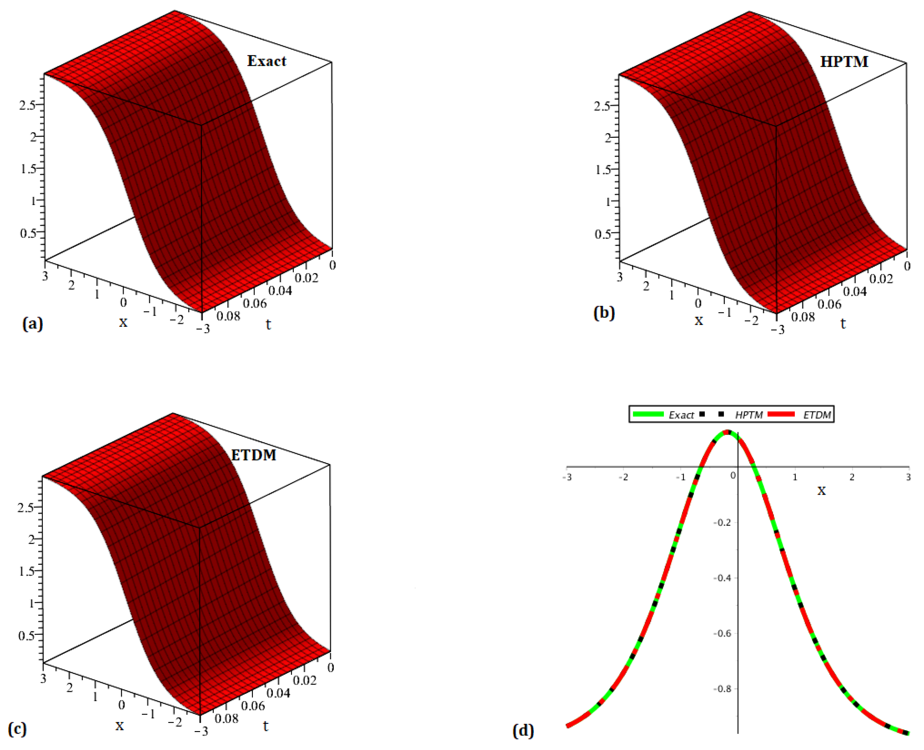
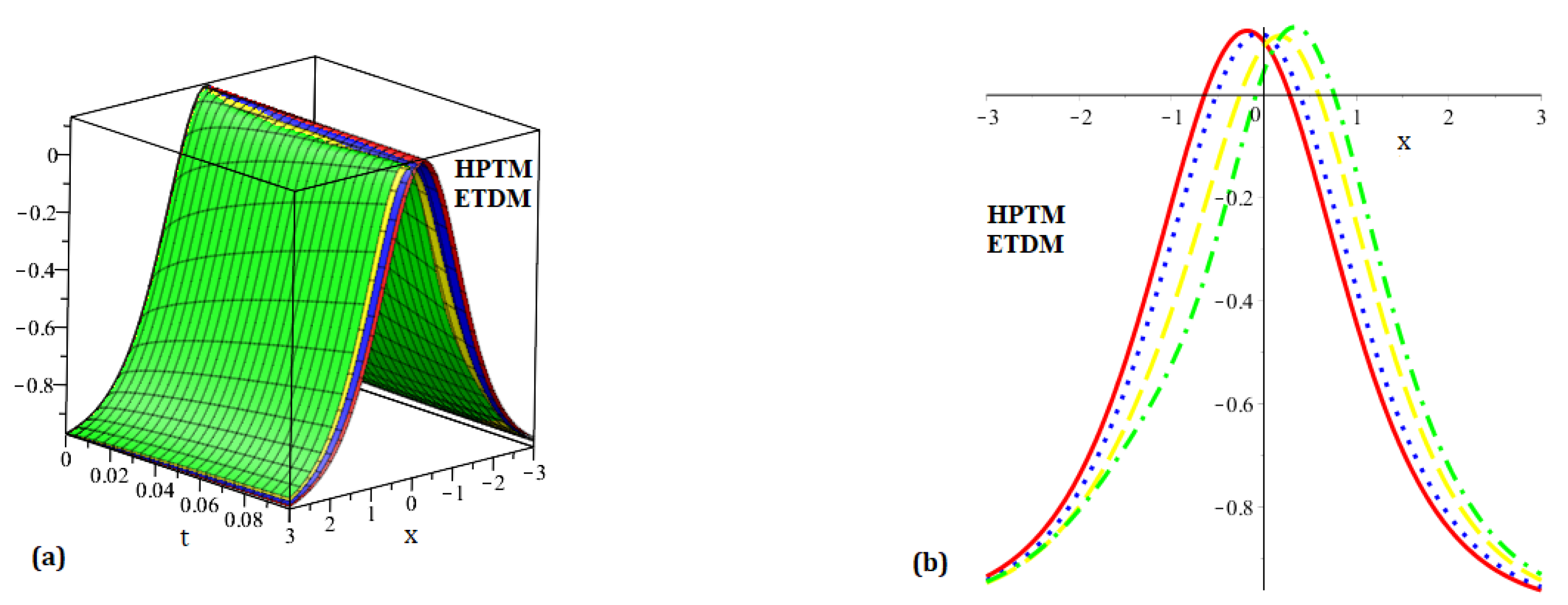
Four diagrams are shown in Figure 7: (a) the precise solution of $\mathrm{f}(\mathrm{x},\mathrm{t})$, (b) representing the HPTM solution of $\mathrm{f}(\mathrm{x},\mathrm{t})$, (c) representing the ETDM solution of $\mathrm{f}(\mathrm{x},\mathrm{t})$, and (d) representing the 2D comparison of the precise and proposed schemes solution for $\mathrm{f}(\mathrm{x},\mathrm{t})$. Figure 8 is split into two sections: the solutions for the suggested strategies are (a) at $\delta =0.6$ and (b) at $\delta =0.8$. Similarly, Figure 9 presents two diagrams: (a) the 3D surface solution of the suggested methods and (b) the 2D surface solution of the suggested methods of $\mathrm{f}(\mathrm{x},\mathrm{t})$. In a similar way, four diagrams are shown in Figure 10: (a) the precise solution of $\mathrm{g}(\mathrm{x},\mathrm{t})$, (b) representing the HPTM solution of $\mathrm{g}(\mathrm{x},\mathrm{t})$, (c) representing the ETDM solution of $\mathrm{g}(\mathrm{x},\mathrm{t})$, and (d) representing the 2D comparison of the precise and proposed schemes solution for $\mathrm{g}(\mathrm{x},\mathrm{t})$. Figure 11 is split into two sections: the solutions for the suggested strategies are (a) at $\delta =0.6$ and (b) at $\delta =0.8$. Similarly, Figure 12 presents two diagrams: (a) the 3D surface solution of the suggested methods and (b) the 2D surface solution of the suggested methods of $\mathrm{g}(\mathrm{x},\mathrm{t})$. The precise results and approximate results achieved by the proposed strategies for $\delta =0.85,0.90,0.95$ and $\delta =1$ are compared in Table 5 and Table 6. The convergence of fractional-order solutions towards integer-order solutions has been confirmed by the graphical and tabular representations. We just compute the iteration up to three terms, and our solution series swiftly converges to the exact result. To increase the approximate outcomes accuracy, a few additional iterations can be examined. The similarity of the results obtained validates the accuracy of the suggested strategies.

Figure 7. Plot (a) representing the precise solution, (b) HPTM solution, (c) ETDM solution, and (d) representing the comparison of the precise and proposed schemes solution for $\mathrm{f}(\mathrm{x},\mathrm{t})$.

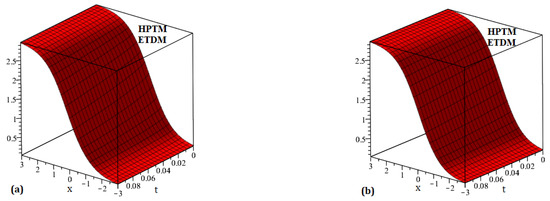
Figure 8. Plot (a) representing our approaches solution at $\delta =0.6$, (b) representing our approaches solution at $\delta =0.8$ for $\mathrm{f}(\mathrm{x},\mathrm{t})$.

Figure 9. Plot (a) representing 3D behavior of our approaches solution (b) representing 2D behavior of our approaches solution at different orders of $\delta =0.4,0.6,0.8,1$ for $\mathrm{f}(\mathrm{x},\mathrm{t})$.

Figure 10. Plot (a) representing the precise solution, (b) HPTM solution, (c) ETDM solution, and (d) representing the comparison of the precise and proposed schemes solution for $\mathrm{g}(\mathrm{x},\mathrm{t})$.

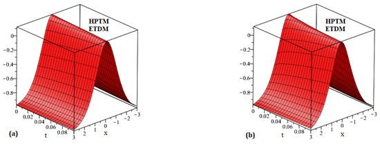
Figure 11. Plot (a) representing our approaches solution at $\delta =0.6$, (b) representing our approaches solution at $\delta =0.8$ for $\mathrm{g}(\mathrm{x},\mathrm{t})$.

Figure 12. Plot (a) representing 3D behavior of our approaches solution (b) representing 2D behavior of our approaches solution at different orders of $\delta =0.4,0.6,0.8,1$ for $\mathrm{g}(\mathrm{x},\mathrm{t})$.

Table 5. Numerical representation of the precise and our approaches solution for $\mathrm{f}(\mathrm{x},\mathrm{t})$.

$\mathbf{t}$	$\mathbf{x}$	$\mathit{\delta }=0.85$	$\mathit{\delta }=0.90$	$\mathit{\delta }=0.95$	$\mathit{\delta }=1$ (Appro)	$\mathit{\delta }=1$ (Exact)	$\mathit{\delta }=1$ (Error)
	0.0	0.6212187486	0.6214906374	0.6217042030	0.6218716422	0.6218716423	1.000000000 $\times {10}^{-10}$
	0.2	0.6444483848	0.6447131499	0.6449211053	0.6450841376	0.6450841376	0.0000000000000
0.01	0.4	0.6670170245	0.6672736736	0.6674752408	0.6676332571	0.6676332571	0.0000000000000
	0.6	0.6888447873	0.6890924668	0.6892869767	0.6894394532	0.6894394530	2.000000000 $\times {10}^{-10}$
	0.8	0.7098640809	0.7101020819	0.7102889792	0.7104354810	0.7104354810	0.0000000000000
	1	0.7300199762	0.7302477367	0.7304265814	0.7305667650	0.7305667650	0.0000000000000
	0.0	0.6192994288	0.6198531806	0.6203133115	0.6206951914	0.6206951914	0.0000000000000
	0.2	0.6425789196	0.6431184078	0.6435667139	0.6439385559	0.6439385560	1.000000000 $\times {10}^{-10}$
0.03	0.4	0.6652044551	0.6657276375	0.6661623278	0.6665228333	0.6665228332	1.000000000 $\times {10}^{-10}$
	0.6	0.6870951836	0.6876002972	0.6880199133	0.6883678769	0.6883678768	1.000000000 $\times {10}^{-10}$
	0.8	0.7081824931	0.7086680680	0.7090713960	0.7094058153	0.7094058152	1.000000000 $\times {10}^{-10}$
	1	0.7284104181	0.7288752834	0.7292613573	0.7295814362	0.7295814362	0.0000000000000
	0.0	0.6175763673	0.6183285204	0.6189704734	0.6195172196	0.6195173196	0.0000000000000
	0.2	0.6408999140	0.6416330073	0.6422585524	0.6427912241	0.6427913242	1.000000000 $\times {10}^{-10}$
0.05	0.4	0.6635758880	0.6642871204	0.6648938791	0.6654105586	0.6654105588	2.000000000 $\times {10}^{-10}$
	0.6	0.6855225729	0.6862095191	0.6867953348	0.6872942801	0.6872942802	1.000000000 $\times {10}^{-10}$
	0.8	0.7066704457	0.7073310765	0.7078944323	0.7083739909	0.7083739910	1.000000000 $\times {10}^{-10}$
	1	0.7269626128	0.7275953039	0.7281347285	0.7285938426	0.7285938428	2.000000000 $\times {10}^{-10}$

Table 6. Numerical representation of the precise and our approaches solution for $\mathrm{g}(\mathrm{x},\mathrm{t})$.

$\mathbf{t}$	$\mathbf{x}$	$\mathit{\delta }=0.85$	$\mathit{\delta }=0.90$	$\mathit{\delta }=0.95$	$\mathit{\delta }=1$ (Appro)	$\mathit{\delta }=1$ (Exact)	$\mathit{\delta }=1$ (Error)
	0.0	−0.8823471142	−0.8823800363	−0.8824059711	−0.8824263486	−0.8824263486	0.0000000000000
	0.2	−0.8854327834	−0.8854709940	−0.8855010772	−0.8855247034	−0.8855247035	1.000000000 $\times {10}^{-10}$
0.01	0.4	−0.8889474516	−0.8889902843	−0.8890239912	−0.8890504544	−0.8890504544	0.0000000000000
	0.6	−0.8928312777	−0.8928780207	−0.8929147917	−0.8929436531	−0.8929436532	1.000000000 $\times {10}^{-10}$
	0.8	−0.8970215594	−0.8970714795	−0.8971107385	−0.8971415458	−0.8971415458	0.0000000000000
	1	−0.9014546801	−0.9015070442	−0.9015482149	−0.9015805166	−0.9015805166	0.0000000000000
	0.0	−0.8821169699	−0.8821827459	−0.8822377760	−0.8822836646	−0.8822836646	0.0000000000000
	0.2	−0.8851651264	−0.8852417744	−0.8853058122	−0.8853591540	−0.8853591540	0.0000000000000
0.03	0.4	−0.8886469628	−0.8887331398	−0.8888050644	−0.8888649271	−0.8888649270	1.000000000 $\times {10}^{-10}$
	0.6	−0.8925029621	−0.8925972288	−0.8926758414	−0.8927412285	−0.8927412285	0.0000000000000
	0.8	−0.8966705829	−0.8967714520	−0.8968555144	−0.8969253977	−0.8969253977	0.0000000000000
	1	−0.9010862160	−0.9011921955	−0.9012804676	−0.9013538180	−0.9013538180	0.0000000000000
	0.0	−0.8819140022	−0.8820017099	−0.8820772985	−0.8821421948	−0.8821421948	0.0000000000000
	0.2	−0.8849281965	−0.8850307991	−0.8851190436	−0.8851946812	−0.8851946811	1.000000000 $\times {10}^{-10}$
0.05	0.4	−0.8883802308	−0.8884959228	−0.8885952736	−0.8886803266	−0.8886803265	1.000000000 $\times {10}^{-10}$
	0.6	−0.8922108917	−0.8923377318	−0.8924465260	−0.8925395737	−0.8925395737	0.0000000000000
	0.8	−0.8963577949	−0.8964937704	−0.8966102864	−0.8967098601	−0.8967098601	0.0000000000000
	1	−0.9007573493	−0.9009004363	−0.9010229459	−0.9011275725	−0.9011275725	0.00000000E+00

8. Conclusions

We prove that our methods for fractional models are clear-cut and accurate, and researchers can apply these methods to tackle a wide range of issues. In this study, we successfully apply two innovative methods to give an approximation solution for NFDE systems with a generalised fractional derivative. We put the approaches to the test in two distinct scenarios. The generated results are shown as a series and, due to their quick convergence, the pace of convergence reveals some remarkable insights. The tables and plots show that the suggested strategies are more accurate and successful than the other approaches. To verify the viability and accuracy of these proposed methodologies, we compare our obtained numerical results with the exact solution. We observe that the fractal solution yields the exact solution only after a few iterations. The use of fractional orders has led to the creation of several different solutions. These solutions have been understood through a variety of representations, which have made clear some important characteristics of the fractional models under investigation. It has been observed that when the arbitrary order becomes closer to integer order, the test issues’ findings converge to the integer-order solution. The numerical findings demonstrate conclusively that the suggested procedures are simple to implement and provide accurate outcomes for the suggested systems. The mathematical results demonstrate the precision, dependability, and effectiveness of the suggested methods, and they can be a useful tool for resolving non-integer order DE that arises in the applied sciences.

References

- Mainardi, F. Fractional Calculus and Waves in Linear Viscoelasticity: An Introduction to Mathematical Models; World Scientific: Singapore, 2022. [Google Scholar]
- Li, C.; Deng, W. Remarks on fractional derivatives. Appl. Math. Comput. 2007, 187, 777–784. [Google Scholar] [CrossRef]
- Alam, M.N.; Ilhan, O.A.; Manafian, J.; Asjad, M.I.; Rezazadeh, H.; Baskonus, H.M.; Macias-Diaz, J.E. New Results of Some of the Conformable Models Arising in Dynamical Systems. Adv. Math. Phys. 2022, 2022, 7753879. [Google Scholar] [CrossRef]
- Alam, M.N.; Ilhan, O.A.; Uddin, M.S.; Rahim, M.A. Regarding on the Results for the Fractional Clannish Random Walker’s Parabolic Equation and the Nonlinear Fractional Cahn-Allen Equation. Adv. Math. Phys. 2022, 2022, 5635514. [Google Scholar] [CrossRef]
- Narahari Achar, B.N.; Lorenzo, C.F.; Hartley, T.T. Initialization issues of the Caputo fractional derivative. Int. Des. Eng. Tech. Conf. Comput. Inf. Eng. Conf. 2005, 47438, 1449–1456. [Google Scholar]
- Miller, K.S.; Ross, B. An Introduction to the Fractional Calculus and Fractional Differential Equations; Wiley: Hoboken, NJ, USA, 1993. [Google Scholar]
- Du, M.L.; Wang, Z.H. Initialized fractional differential equations with Riemann-Liouville fractional-order derivative. Eur. Phys. J. Spec. Top. 2011, 193, 49–60. [Google Scholar] [CrossRef]
- Caputo, M.; Fabrizio, M. A new defnition of fractional derivative without singular kernel. Prog. Fract. Difer. Appl. 2016, 1, 73–85. [Google Scholar]
- Atangana, A.; Baleanu, D. New fractional derivatives with non-local and nonsingular kernel theory and application to heat transfer model. Therm. Sci. 2016, 20, 763–769. [Google Scholar] [CrossRef]
- Dubey, R.S.; Belgacem, F.B.M.; Goswami, P. Homotopy perturbation approximate solutions for Bergman’s minimal blood glucose-insulin model. Fractal Geom. Nonlinear Anal. Med. Biol. 2016, 2, 1–6. [Google Scholar]
- Baleanu, D.; Guvenc, Z.B.; Machado, J.A.T. New Trends in Nanotechnology and Fractional Calculus Applications; Springer: Berlin/Heidelberg, Germany, 2010; Volume 10, pp. 978–990. [Google Scholar]
- Nasrolahpour, H. A note on fractional electrodynamics. Commun. Nonlinear Sci. Numer. Simul. 2013, 18, 2589–2593. [Google Scholar] [CrossRef]
- Baleanu, D.; Wu, G.C.; Zeng, S.D. Chaos analysis and asymptotic stability of generalized Caputo fractional differential equations. Chaos Solitons Fractals 2017, 102, 99–105. [Google Scholar] [CrossRef]
- Kumar, D.; Seadwy, A.R.; Joarder, A.K. Modified Kudryashov method via new exact solutions for some conformable fractional differential equations arising in mathematical biology. Chin. J. Phys. 2018, 56, 75–85. [Google Scholar] [CrossRef]
- Drapaca, C.S.; Sivaloganathan, S. A fractional model of continuum mechanics. J. Elast. 2012, 107, 105–123. [Google Scholar] [CrossRef]
- Agarwal, P.; El-sayed, A.A. Non-standard finite difference and Chebyshev collocation methods for solving fractional diffusion equation. Phys. A 2018, 500, 40–49. [Google Scholar] [CrossRef]
- Sunthrayuth, P.; Alyousef, H.A.; El-Tantawy, S.A.; Khan, A.; Wyal, N. Solving Fractional-Order Diffusion Equations in a Plasma and Fluids via a Novel Transform. J. Funct. Spaces 2022, 2022, 1899130. [Google Scholar] [CrossRef]
- Shrahili, M.; Dubey, R.S.; Shafay, A. Inclusion of fading memory to banister model of changes in physical condition. Discret. Contin. Dyn. Syst. Ser. S 2020, 13, 881–888. [Google Scholar] [CrossRef]
- Vieru, D.; Fetecau, C.; Shah, N.A.; Yook, S.J. Unsteady natural convection flow due to fractional thermal transport and symmetric heat source/sink. Alex Eng. J. 2023, 64, 761–770. [Google Scholar] [CrossRef]
- Ray, S.S.; Atangana, A.; Noutchie, S.C.O.; Kurulay, M.; Bildik, N. Fractional calculus and its applications in applied mathematics and other sciences. Math. Prob. Eng. 2014, 2014, 849395. [Google Scholar] [CrossRef]
- Roozi, A.; Alibeiki, E.; Hosseini, S.S.; Shafiof, S.M.; Ebrahimi, M. Homotopy perturbation method for special nonlinear partial differential equations. J. King Saud Uni. (Sci.) 2011, 23, 99–103. [Google Scholar] [CrossRef]
- Ganie, A.H.; Khan, A.; Alhamzi, G.; Saeed, A.M. A new solution of the nonlinear fractional logistic differential equations utilizing efficient techniques. AIP Adv. 2024, 14, 035134. [Google Scholar] [CrossRef]
- Ganie, A.H.; Mofarreh, F.; Khan, A. A novel analysis of the time-fractional nonlinear dispersive K (m, n, 1) equations using the homotopy perturbation transform method and Yang transform decomposition method. AIMS Math. 2024, 9, 1877–1898. [Google Scholar] [CrossRef]
- Zayed, E.M.; Amer, Y.A.; Al-Nowehy, A.G. The modified simple equation method and the multiple exp-function method for solving nonlinear fractional Sharma-Tasso-Olver equation. Acta Math. Appl. Sin. Engl. Ser. 2016, 32, 793–812. [Google Scholar] [CrossRef]
- Khan, M.; Gondal, M.A.; Hussain, I.; Vanani, S.K. A new comparative study between homotopy analysis transform method and homotopy perturbation transform method on a semi infinite domain. Math. Comput. Model. 2012, 55, 1143–1150. [Google Scholar] [CrossRef]
- Fadhal, E.; Ganie, A.H.; Alharthi, N.S.; Khan, A.; Fathima, D.; Elamin, A.E.A. On the analysis and deeper properties of the fractional complex physical models pertaining to nonsingular kernels. Sci. Rep. 2024, 14, 22182. [Google Scholar] [CrossRef] [PubMed]
- Fathima, D.; Alahmadi, R.A.; Khan, A.; Akhter, A.; Ganie, A.H. An efficient analytical approach to investigate fractional Caudrey-Dodd-Gibbon Equations with non-singular kernel derivatives. Symmetry 2023, 15, 850. [Google Scholar] [CrossRef]
- Feng, L.B.; Zhuang, P.; Liu, F.; Turner, I.; Gu, Y. Finite element method for space-time fractional diffusion equation. Numer. Algorithms 2016, 72, 749–767. [Google Scholar] [CrossRef]
- Ismail, G.M.; Abdl-Rahim, H.R.; Ahmad, H.; Chu, Y.M. Fractional residual power series method for the analytical and approximate studies of fractional physical phenomena. Open Phys. 2020, 18, 799–805. [Google Scholar] [CrossRef]
- Mirzaee, F.; Rezaei, S.; Samadyar, N. Solution of time-fractional stochastic nonlinear sine-Gordon equation via finite difference and meshfree techniques. Math. Methods Appl. Sci. 2022, 45, 3426–3438. [Google Scholar] [CrossRef]
- Zada, L.; Nawaz, R.; Jamshed, W.; Ibrahim, R.W.; Tag El Din, E.S.M.; Raizah, Z.; Amjad, A. New optimum solutions of nonlinear fractional acoustic wave equations via optimal homotopy asymptotic method-2 (OHAM-2). Sci. Rep. 2022, 12, 18838. [Google Scholar] [CrossRef]
- Mirzaee, F.; Rezaei, S.; Samadyar, N. Application of combination schemes based on radial basis functions and finite difference to solve stochastic coupled nonlinear time fractional sine-Gordon equations. Comput. Appl. Math. 2022, 41, 10. [Google Scholar] [CrossRef]
- Kamil Jassim, H.; Vahidi, J. A new technique of reduce differential transform method to solve local fractional PDEs in mathematical physics. Int. J. Nonlinear Anal. Appl. 2021, 12, 37–44. [Google Scholar]
- Chavada, A.; Pathak, N.; Khirsariya, S.R. A fractional mathematical model for assessing cancer risk due to smoking habits. Math. Model. Control 2024, 4, 246–259. [Google Scholar] [CrossRef]
- Awadalla, M.; Ganie, A.H.; Fathima, D.; Khan, A.; Alahmadi, J. A mathematical fractional model of waves on Shallow water surfaces: The Korteweg-de Vries equation. AIMS Math. 2024, 9, 10561–10579. [Google Scholar] [CrossRef]
- Moumen, A.; Shafqat, R.; Alsinai, A.; Boulares, H.; Cancan, M.; Jeelani, M.B. Analysis of fractional stochastic evolution equations by using Hilfer derivative of finite approximate controllability. AIMS Math. 2023, 8, 16094–16114. [Google Scholar] [CrossRef]
- Farid, S.; Nawaz, R.; Shah, Z.; Islam, S.; Deebani, W. New iterative transform method for time and space fractional (n+1)-dimensional heat and wave type equations. Fractals 2021, 29, 2150056. [Google Scholar] [CrossRef]
- Ullah, H.; Fiza, M.; Khan, I.; Mosa, A.A.A.; Islam, S.; Mohammed, A. Modifications of the optimal auxiliary function method to fractional order fornberg-whitham equations. CMES-Comput. Model. Eng. Sci. 2023, 136, 277–291. [Google Scholar] [CrossRef]
- Boiti, M.; Leon, J.J.; Pempinelli, F. Spectral transform for a two spatial dimension extension of the dispersive long wave equation. Inverse Probl. 1987, 3, 371. [Google Scholar] [CrossRef]
- Adomian, G. Nonlinear Stochastis System Theory and Applications to Physics; Kluwer Academic Publishers: Dordrecht, The Netherlands, 1989. [Google Scholar]
- Adomian, G. Solving Frontier Problems of Physics: The Decomposition Method; Springer: Dordrecht, The Netherlands, 1994. [Google Scholar]
- He, J.H. Homotopy perturbation technique. Comput. Methods Appl. Mech. Engrg. 1999, 178, 257–262. [Google Scholar] [CrossRef]
- He, J.H. A coupling method of a homotopy technique and a perturbation technique for non-linear problems. Int. J.-Non-Linear Mech. 2000, 35, 37–43. [Google Scholar] [CrossRef]
- He, J.H. Homotopy perturbation method: A new nonlinear analytical technique. Appl. Math. Comput. 2003, 135, 73–79. [Google Scholar] [CrossRef]
- Neamaty, A.; Agheli, B.; Darzi, R. Applications of homotopy perturbation method and Elzaki transform for solving nonlinear partial differential equations of fractional order. J. Nonlin. Evolut. Equat. Appl. 2016, 2015, 91–104. [Google Scholar]
- Ganie, A.H.; AlBaidani, M.M.; Khan, A. A comparative study of the fractional partial differential equations via novel transform. Symmetry 2023, 15, 1101. [Google Scholar] [CrossRef]
- Jena, R.M.; Chakraverty, S. Solving time-fractional Navier-Stokes equations using homotopy perturbation Elzaki transform. SN Appl. Sci. 2019, 1, 16. [Google Scholar] [CrossRef]
- Sedeeg, A.K.H. A coupling Elzaki transform and homotopy perturbation method for solving nonlinear fractional heat-like equations. Am. J. Math. Comput. Model 2016, 1, 15–20. [Google Scholar]
- Elzaki, T.M. On the connections between Laplace and Elzaki transforms. Adv. Theor. Appl. Math. 2011, 6, 1–11. [Google Scholar]
Disclaimer/Publisher’s Note: The statements, opinions and data contained in all publications are solely those of the individual author(s) and contributor(s) and not of MDPI and/or the editor(s). MDPI and/or the editor(s) disclaim responsibility for any injury to people or property resulting from any ideas, methods, instructions or products referred to in the content. |
© 2024 by the authors. Licensee MDPI, Basel, Switzerland. This article is an open access article distributed under the terms and conditions of the Creative Commons Attribution (CC BY) license (https://creativecommons.org/licenses/by/4.0/).