Abstract
Two rheological Burgers–Faraday models and rheological dynamical systems were created by using two new rheological models: Kelvin–Voigt–Faraday fractional-type model and Maxwell–Faraday fractional-type model. The Burgers–Faraday models described in the paper are new models that examine the dynamical behavior of materials with coupled fields: mechanical stress and strain and the electric field of polarization through the Faraday element. The analysis of the constitutive relation of the fractional order for Burgers–Faraday models is given. Two Burgers–Faraday fractional-type dynamical systems were created under certain approximations. Both rheological Burgers-Faraday dynamic systems have two internal degrees of freedom, which are introduced into the system by each standard light Burgers-Faraday bonding element. It is shown that the sequence of bonding elements in the structure of the standard light Burgers-Faraday bonding element changes the dynamic properties of the rheological dynamic system, so that in one case the system behaves as a fractional-type oscillator, while in the other case, it exhibits a creeping or pulsating behavior under the influence of an external periodic force. These models of rheological dynamic systems can be used to model new natural and synthetic biomaterials that possess both viscoelastic/viscoplastic and piezoelectric properties and have dynamical properties of stress relaxation.
Keywords:
rheological models of fractional type with piezo-electrical properties; viscous fluid; Burgers–Faraday fractional-type model; rheological Burgers–Faraday dynamical system; oscillator of fractional type with piezoelectric properties; creeper of fractional type with piezoelectric properties; stress relaxation; inner degree of freedom; biomaterials 1. Introduction
Numerous natural and synthetic materials exhibit viscoelastic/viscoplastic properties and those with purely piezoelectric properties. However, materials that possess both properties exhibit the most intriguing dynamic. Modeling such complex behavior is a real challenge.
The stress problems of piezoceramic plates were studied in [1,2,3,4]. Additionally, rheological models exist for various materials [5], including construction materials [6,7], textiles [8], living materials [9,10,11], and thermomechanical systems [12]. Among the most commonly used models for representing the viscoelastic and viscoplastic properties of materials are the Maxwell and Kelvin–Voigt models, often enhanced with fractional calculus, as well as the Zener model (also known as the Standard Linear Solid (SLS) model) [13]. Materials exhibiting both viscoelastic/viscoplastic and piezoelectric properties include elastomers, certain types of polymers and some composites [14,15], metals at high temperatures and biomaterials. It is known for a long time that hard tissues of living organisms can generate electrical potentials in response to mechanical stress- or any stress deforming their structure [16]. Biological materials with such properties include bones [17,18] tendons, cartilage, hairs, silk, paper, natural polymers such as cellulose, fibroin, keratin, collagen, DNA, RNA, myosin, as well as artificial polymers like acetylcellulose, polycaprolactane and polymethyl-l-glutamate. Bones, for instance, exhibit stress-induced electrical effects in both bending and compression modes. These piezoelectric properties of the bones were first studied decades ago [19]. At that time, it was hypothesized that surface charges on stressed bone may be the controlling factor in bone formation which was proven in other studies [20,21,22,23]. Fractional order derivatives have been widely used in modeling the dynamical responses of various structures [24,25]. For example, fractional Maxwell models have been used to describe small strains in porcine urinary bladders during initial stages [26]. For multi-step relaxation under large strains, a fractional-type quasi-linear viscoelastic model combining a Scott–Blair relaxation function and an exponential instantaneous stress response was used [26]; a class of return mapping algorithms for fractional-type visco-elasto-plasticity was developed by using canonical combinations of Scott–Blair elements to construct a series of well-known fractional linear viscoelastic models, such as Kelvin–Voigt, Maxwell, Kelvin–Zener, and Poynting–Thomson [27]. Other applications include modeling relaxation and creep properties in materials such as fractal ladders and [28] for bio-thermomechanical problems in functionally graded anisotropic nonlinear viscoelastic soft tissues [29].
For studying thermo-mechanical interactions in living tissues during hyperthermia treatment by using fractional time derivatives and Laplace transform techniques to the generalized bio-thermo-elastic model and eigenvalue approach [30]. For 3D printed material with creep properties fractional models have also been utilized [31]. A novel AEF–Zener model of viscoelastic dampers incorporating temperature effects and the fractional-order equivalence principle was proposed in [13]. Fractional-order iterative methods were used to model the viscoelasticity and stiffening effects of dielectric elastomer considering both the strain-stiffening and viscoelasticity effects within electromechanical coupling in dielectric elastomer [32]. Recently, Xu et al. [33] proposed a high-accuracy unique fractional-order model that can capture hysteresis and creep nonlinear characteristics such as piezoelectric lag, non-local memory, peak transition, and creep amplitude–frequency features in piezoelectric actuators. A comprehensive and unified theory of analytical dynamics for discrete hereditary systems is presented in [34], along with experimental methods to determine the kernel of rheology for various hereditary properties of rheological materials. Furthermore, a generalized fractional-type dissipation function for system energy and an extended Lagrangian differential equation in matrix form for fractional-type discrete dynamical systems are introduced in [24,35].
Finally, an important question posed in [36] remains highly relevant: “Does a Fractal Microstructure Require a Fractional Viscoelastic Model?” [36].
The aim of this work is to create new rheological models using fractional order derivatives that can be used to model the behavior of biomaterial with piezo-electrical and viscoelastic properties by integrating the Maxwell or Kelvin–Voigt element both with fractional-type properties with the Faraday element. In the era of synthesizing new materials for modern industry and robotics, materials with such properties will be increasingly synthesized and used, so it is necessary to understand their mechanical and electrical properties as well as the coupled fields and interactions of these future materials. In the following chapters, we will first describe the simpler Kelvin–Voigt–Faraday fractional-type model and its behavior in a special case, followed by the Maxwell–Faraday fractional-type model and its behavior in a special case, and then the two complex Burgers–Faraday models as well as Burgers-Faraday dynamic systems composed of the corresponding types of Burgers–Faraday models. We will also examine the dynamics of these dynamic systems depending on the order of the element connections in the system. A current trend in science is to create complex materials alongside their mathematical and mechanical models which can describe their complex behavior that depends on coupled fields. In this paper, we will present new models that can address this problem.
2. Methodology
2.1. Complex Faraday Fractional-Type Models
In this section, two complex rheological Burgers–Faraday fractional-type models are presented, and their differential constitutive relation of fractional order as well as the dynamics of both models for some special cases.
By connecting a Faraday element, which represents a material with ideal elastic and piezoelectric properties, in parallel with a Kelvin–Voigt fractional-type element, we obtain the Kelvin–Voigt–Faraday fractional-type model (KVFYF). If the Faraday element is connected to a series with the Maxwell fractional-type model, we obtain the Maxwell–Faraday fractional-type model (MFYF), as shown in Figure 1.
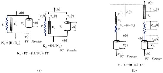
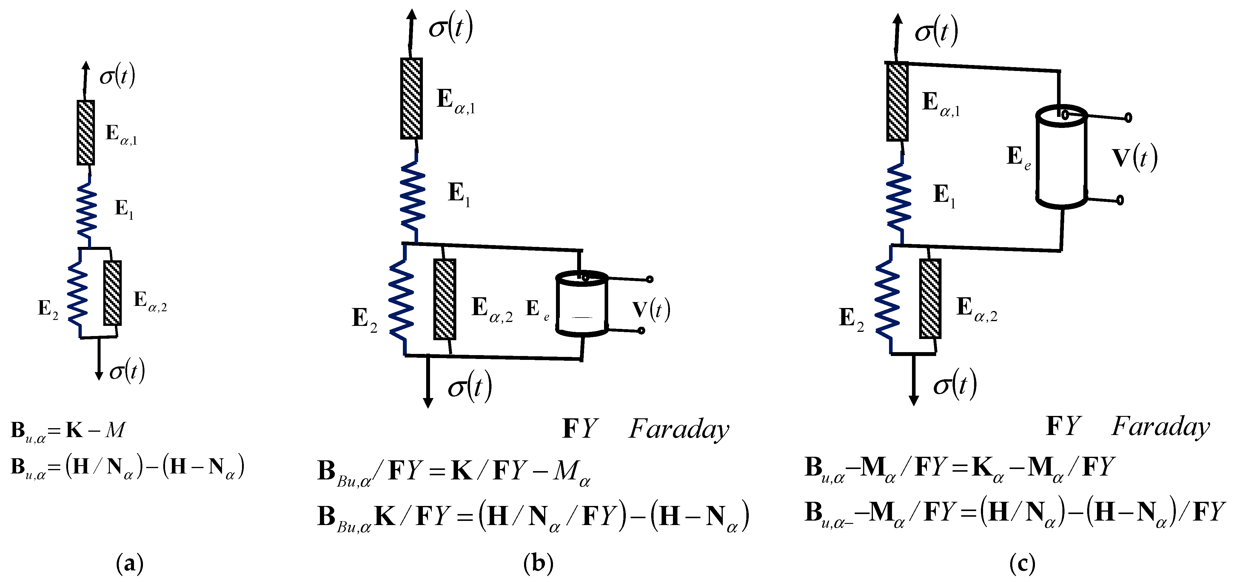
Figure 1.
(a) Kelvin–Voigt–Faraday fractional-type model. (b) Maxwell–Faraday fractional-type model. H—Hook ideally elastic element. N—Newton ideally viscous fluid (fractional derivative is introduced in this element to describe viscoelastic nature of the material). FY—Faraday element with ideally elastic and piezoelectric properties. K—Kelvin–Voigt element. M—Maxwell element.
2.1.1. The Dynamical Properties of the Kelvin–Voigt–Faraday Fractional-Type Model
Kelvin–Voigt–Faraday fractional-type model represents a rheological model of the solids. The Kelvin–Voigt fractional-type model is connected in parallel with the Faraday model. In the Kelvin–Voigt fractional-type model Hook element is represented by the ideally elastic spring and the Newton element is presented as an ideally viscous fluid where a fractional order derivative is introduced to describe the viscoelastic nature of the material. Figure 1a represents a fictive cross-section of the model with component normal stresses of each consecutive element in parallel in the model.
The resultant normal stress at the end of the Kelvin–Voigt–Faraday fractional-type model is as follows:
where is the normal stress in the Hook element; is the normal stress in the Newton ideally viscous fluid with fractional type properties; is the normal stress in the Faraday element, is a differential operator of Caputo type, as shown in Equation (2).
where is Gamma function as follows:
where is determined experimentally. When exponent of the fractional order differentiation is , the application of the fractional order derivative gives the time function which represents dilatation.
When , the application of the fractional order derivative gives the first derivative of time function. These properties of the differential operator of the fractional order, when its fractional exponent takes values as rational numbers within an interval , including its boundary values, allow us to define both integer-order derivatives and fractional-order derivatives with a single expression. This provides a useful mathematical description in various applications.
Equation (1) represents a differential constitutive fractional-type relation that connect normal stress and axial dilatation , and axial dilatation rate in the Kelvin–Voigt–Faraday fractional-type model and can be rewritten as follows:
The electric voltage in the Faraday element that is generated as a result of polarization closed by mechanical loading in the Faraday element.
Dielectric displacement in Faraday element is in linear relation with normal stress and axial dilatation: and .
2.1.2. The Dynamical Behavior of the Kelvin–Voigt–Faraday Fractional-Type Model in a Special Case
We will study the behavior of the Kelvin–Voigt–Faraday fractional-type model in the special case when the model is in the steady state or under very slow change in the dynamical load. Then, the axial dilatation rate of the fractional-type tends to be zero and the material behaves as a basic ideally elastic material, and the normal stress of the material is almost proportional to the axial dilatation . In that case Equation (1) becomes
If the normal stress at the end of the Kelvin–Voigt–Faraday fractional-type model suddenly increases from zero to some finite value , and remains constant during the subsequent time interval, than .
In that case to solve/define axial dilatation as a time function in the Kelvin–Voigt–Faraday fractional-type model we applied Laplace transform on , and obtained the following:
As , , and, ,
It follows:
The axial dilatation of the Kelvin–Voigt–Faraday fractional-type model (KVFYF) as a time function is then inverse Laplace transform of algebra Equation (8):
To find the time domain of the inverse Laplace transform of algebra Equation (8) which represents an approximatively analytical expression for axial dilatation of KVFYF as a time function, it is necessary to expand expression into a series in powers of p, which is a complex number, using the formula for approximate series expansion (see Ref. [35]):
As
The inverse Laplace transform of expression (10) is as follows:
and is related to axial dilatation in time
Dielectric displacement , and , for the special case of constant normal stress , in Faraday-element is:
In the case of constant normal stress the Kelvin–Voigt–Faraday fractional-type model exhibits the property of delayed elasticity, where axial dilatation lags behind the stress (Figure 2a).
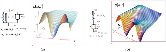
Figure 2.
(a) The surface of the delayed elasticity of the Kelvin–Voigt–Faraday fractional-type model, (b) the surface of normal stress relaxation in the Maxwell–Faraday fractional-type model. Both models exhibit a piezoelectric property.
If we apply the Laplace transform to differential Equation (4) of the fractional order we obtain the following:
Expression (14) is an algebra equation, and represents the product of two Laplace transforms: one Laplace transform of the normal stress and the other in the form of , from which it is concluded that these two functions are also in convolution with the axial dilatation function , which leads to the following:
As , the expression can be expand into a series (see Ref. [35]) and written as follows:
Inverse Laplace transform of (16) is as follows:
Based on the convolution of these three functions, and for which the following holds:
Convolution integral has a following form:
Expression (19) is a constitutive equation related to axial dilatation and normal stress in the Kelvin–Voigt–Faraday fractional-type model.
Electric voltage in Faraday element in the Kelvin–Voigt–Faraday fractional-type model is in the following form:
2.1.3. The Dynamical Properties of the Maxwell–Faraday Fractional-Type Model
The Maxwell–Faraday fractional-type model with structural formula consist of the Newton viscous fractional-type element, the Hooke ideal elastic element, the Faraday ideally elastic, and the piezoelectric element all connected in series (Figure 1b). This Maxwell–Faraday fractional-type model properties are that the axial dilatation ratio of fractional type thought all the model is equal to sum of the axial dilatation ratio of each element (Newton viscous fractional type element), (Hooke ideal elastic element) and (Faraday ideally elastic and piezoelectric element) in series.
Resultant axial dilatation velocity of the Maxwell–Faraday fractional-type model is equal to the following:
Or in the the following form:
Expression (22) represents an inhomogeneous ordinary differential constitutive relation of the fractional order of the Maxwell–Faraday fractional-type model. The following relation is valid:
2.1.4. The Dynamical Behavior of the Maxwell–Faraday Fractional-Type Model in Special Case
For the special case when normal stress is proportional to the dilatation ratio of fractional type:
The material described by the Maxwell–Faraday fractional-type model behaves as a viscoelastic fluid: deformation/axial dilatation increases unlimitedly. Upon unloading of material, axial deformation exists only in the Newton viscous fractional-type element.
If this material is suddenly loaded to a certain value of normal stress, it undergoes elastic deformation, which occurs instantaneously in the Hooke ideally elastic element and the Faraday ideal elastic piezoelectric element. Due to the sudden loading, the flow in the serially connected Newton viscous element of fractional type does not come into effect at the initial moment of observation.
If we prevent the development of deformation/axial dilatation, assuming that the rate of axial dilatation, of fractional type, tends to be zero , then, the normal stress becomes a function of time, which needs to be determined.
To express the normal stress as a time function using approximate analytical expressions when the axial dilatation ratio of the fractional type is constant Laplace transform on expression (23 is performed and then the inverse Laplace using the same procedure that is described previously for finding the approximate analytical expressions for normal stress as a time function in the Kelvin–Voigt–Faraday fractional-type model. The approximate analytical expression for normal stress as a time function in the Maxwell–Faraday fractional-type model for the case when axial dilatation ratio of the fractional type is constant , is in the following form:
The electrical voltage that is induced by stress and polarization in the Faraday element in Maxwell–Faraday fractional-type model is as follows:
Dielectric displacement is as follows:
2.1.5. The Maxwell–Faraday Fractional-Type Model Material Properties
Expression (25) indicates the material properties of normal stress relaxation. In this model, normal stress relaxation is reflected in the decrease in normal stress over time, when the axial strain remains constant over time. The surface of normal stress relaxation for the Maxwell–Faraday fractional-type model is presented in Figure 2b. The studied material, based on a Maxwell–Faraday fractional-type model is a viscoelastic fluid with piezoelectric properties. This model can be used to describe the properties of metals at very high temperatures, while also exhibiting piezoelectric characteristics.
Differential constitutive relation of fractional order (23) can be solved by applying the Laplace transform and then, by expanding into a series by the powers of the complex parameter we obtain the following:
Using the property of three functions that are in convolution, as well as the relationships of their Laplace transforms and the convolution integral, in a similar way as it was described for the Kelvin–Voigt–Faraday fractional-type model we can obtain a constitutive integral equation of the Maxwell–Faraday fractional-type model in the form of integral of convolution:
3. Complex Burgers–Faraday Fractional-Type Models
In this section, we describe complex Burgers–Faraday fractional-type models and their dynamical behavior. The schematic of the Burgers fractional-type model (Figure 3a) and Burgers–Faraday fractional-type models are shown in Figure 3b,c. The Burgers–Faraday fractional-type model presented in Figure 3b is obtained by introducing the Faraday element in parallel connection with the Kelvin–Voigt fractional type element of the Burgers fractional-type model. The Burgers–Faraday fractional-type model presented in Figure 3c is obtained by introducing the Faraday element in parallel connection with the Maxwell fractional-type element of the Burgers fractional-type model. The Burgers fractional-type model (Figure 3a) represents a series of connections between a Maxwell fractional-type element and the Kelvin–Voigt fractional-type element.

Figure 3.
(a) Burgers fractional-type model. (b) Burgers–Faraday fractional-type model—viscous fluid with piezoelectric properties (BFYF VF model) (c) Burgers–Faraday fractional-type model—viscoelastic solid with piezoelectric properties (BFYF VES model). H- Hook ideally elastic element. N—Newton ideally viscous fluid (fractional derivative is introduced in this element to describe viscous nature and fractional-type dissipation energy of the material). FY—Faraday element with ideally elastic and piezoelectric properties. K—Kelvin–Voigt fractional-type element. M-Maxwell fractional-type element. B—Burgers fractional-type element.
3.1. Burgers–Faraday Fractional-Type Model–Viscous Elastic Fluid with Piezoelectric Properties (BFYF CF Model)
The constitutive relation for the Burgers–Faraday fractional-type model (BFYF CF model) is as follows:
The relationship between normal stress and axial strain in BFYF VF classic model is as follows:
For the analogy of the details of the mathematical description and the derivation of the differential constitutive equation, see Reference [37].
The constitutive relations of the BFYF VF model contains time derivatives of fractional order as well as higher-order derivatives. The total axial strain in the CF model is equal to the sum of the component axial strains and of its constituent elements: the Maxwell fractional-type element and the Kelvin–Voigt–Faraday fractional-type element , while the normal stress is the same across all cross-sections of the model’s components . Based on this analysis and the derived conclusions, we can write the following relations:
After differentiating (34) according to from (35) and substitution of terms from (36) constitutive relation of the BFYF VF model is in the following form:
Or
As relation is valid for each part of the BFYF VF model Equations (38) and (39) can be rewritten in the following form:
These last two Relations (40) and (41) between normal stress and axial strain , and their corresponding fractional-order derivatives, are coupled differential constitutive relations of fractional order for the BFYF VF model. Under certain conditions, the model exhibits properties of delayed elasticity and/or normal stress relaxation. From this system of fractional-order differential constitutive Relations (40) and (41), we can eliminate the axial strain rate, fractional order, and obtain a single relation linking normal stress and axial strain in this complex rheological structure by transitioning to the domain of the Laplace transform in the following form:
or
After substituting (45) in (44) we obtain the following:
At the end we obtain the Laplace transform of the normal stress as a function of the Laplace transform of the axial strain for the complex rheological structure of the BFYF VF model in the following form:
Now, by applying the inverse Laplace transform to Equation (47), it is possible to obtain the time function of normal stress from the axial strain of the complex rheological structure of the BFYF VF model using the convolution integral. However, the problem of determining the inverse Laplace transform remains unsolved for now.
3.2. The Burgers–Faraday Fractional-Type Model—Elastoviscous Solid with Piezoelectric Properties (BFYS VES Model)
The BFYF VES model presented in Figure 3c consists of a Maxwell–Faraday fractional-type element (a Maxwell fractional-type element connected in parallel with a Faraday element) connected in a series with a Kelvin–Voigt fractional-type element. The stress and strain will be analyzed in elements of the BFYF VES model and the end in the whole BFYF VES model.
The total stress in the Maxwell–Faraday fractional-type element which is a substructure of the complex BFYF VES model is as follows:
If we apply the Laplace transform to the previous fractional-order constitutive Relation (48), we obtain the following:
Considering the components of the BFYF VES model, the system of constitutive relations of fractional order of the complete BFYF VES model is in the following form:
These fractional-order constitutive relations provide the connections between axial strain and normal stress in the complex rheological BFYF VES model, as well as the normal stresses and axial strains in the substructures of the fractional-type Kelvin–Voigt model and the fractional-type Maxwell-Faraday model.
By applying the Laplace transform to the previous two fractional-order constitutive Relations (51) and (52), we obtain the following relations:
These previous fractional-order constitutive Relations (56) and (57) provide the connections between the Laplace transforms of the normal stress and the Laplace transforms of the axial strain in the complex rheological BFYF VES model, as well as the axial strains and normal stresses in the substructures of the fractional-type Kelvin–Voigt model and the fractional-type Maxwell-Faraday model .
4. Two Rheological Burgers–Faraday Discrete Dynamical Systems of Fractional Type-One Oscillator BFY VES DS and the Other Creeper BFY CF DS Both with Piezoelectric Properties
In this section of the paper, we define two new types of rheological discrete dynamic systems of fractional type and piezoelectric properties, which we have named rheological Burgers–Faraday discrete dynamic systems of fractional type. We introduce the concepts of standard light complex binding elements, and the concept of standard light complex rheological binding elements: the Burgers–Faraday–BFY VES DS and Burgers–Faraday– BFY CF DS standard light binding models. In this part, we will define the rheological Burgers–Faraday discrete dynamic systems consisting of a single material point (rigid body) that moves rectilinearly translatory on a smooth horizontal surface and is connected by one of the standard light rheological Burgers–Faraday (BFY VES DS or BFY CF DS) models to a fixed wall. Such rheological discrete dynamic systems have one external and two internal degrees of freedom. We will study the dynamics of two such rheological Burgers–Faraday discrete dynamic systems: one type is a fractional rheological oscillator with piezoelectric properties (Figure 4), and the other is a creeper of fractional type with piezoelectric properties (Figure 5), each in two variations in the sequence of element connections in the Burgers–Faraday binding models.

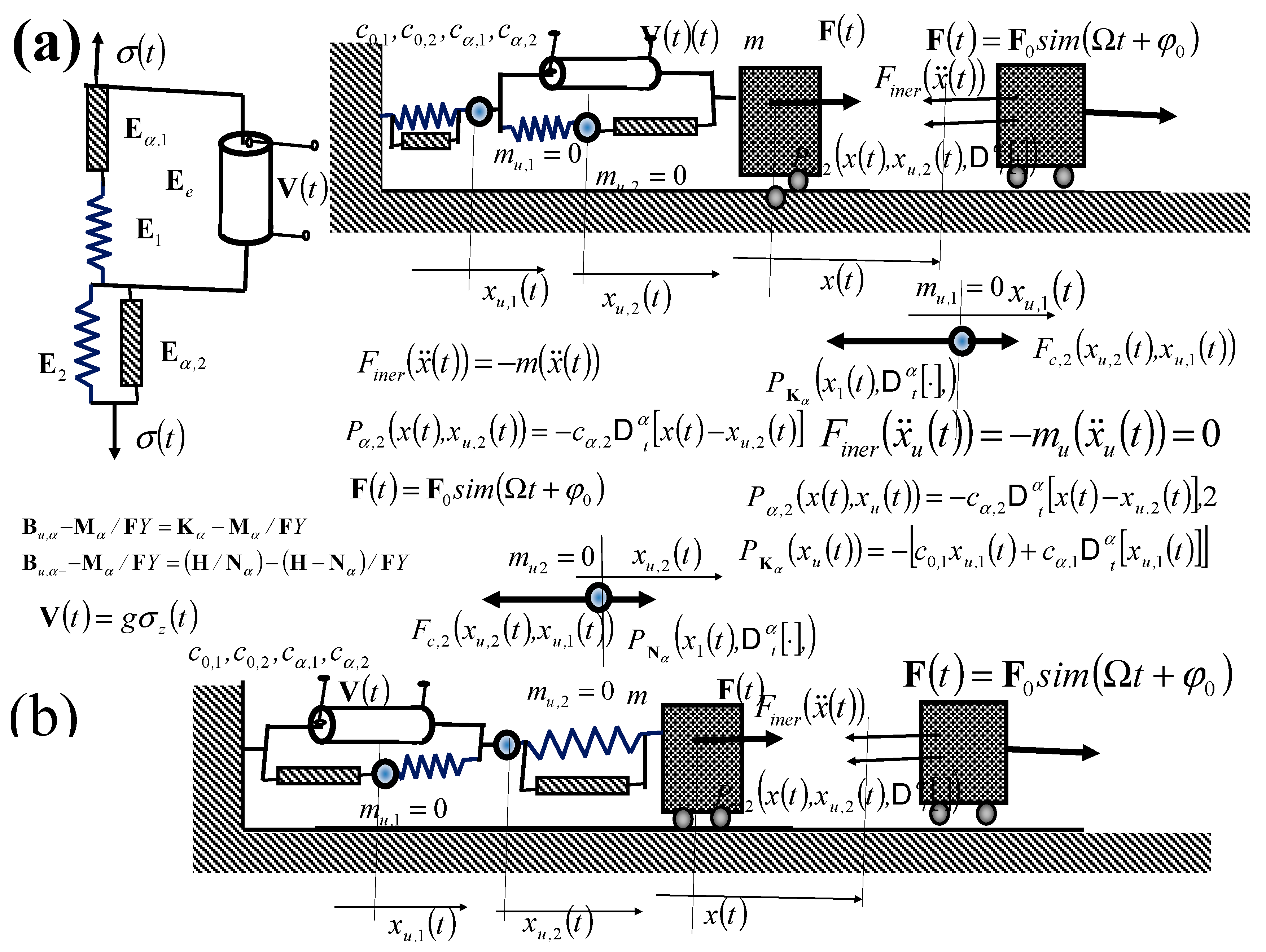
Figure 4.
Burgers–Faraday discrete dynamical system of fractional-type BFY VES DS fractional-type oscillator with piezoelectric properties: (a) A rheological discrete dynamic system consisting of a single material point (rigid body) with mass , connected by a standard light complex Burgers–Faraday–VES rheological model of the ideal fractional type (BFY VES DS, upper part in figure). The system has one external and two internal degrees of freedom. (b) A dynamic rheological system with the reversed sequence of the structure’s connections in the standard light complex ideal Burgers–Faraday model of fractional type (BFY VES DSR, lower part in figure).
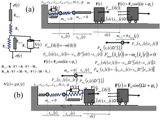
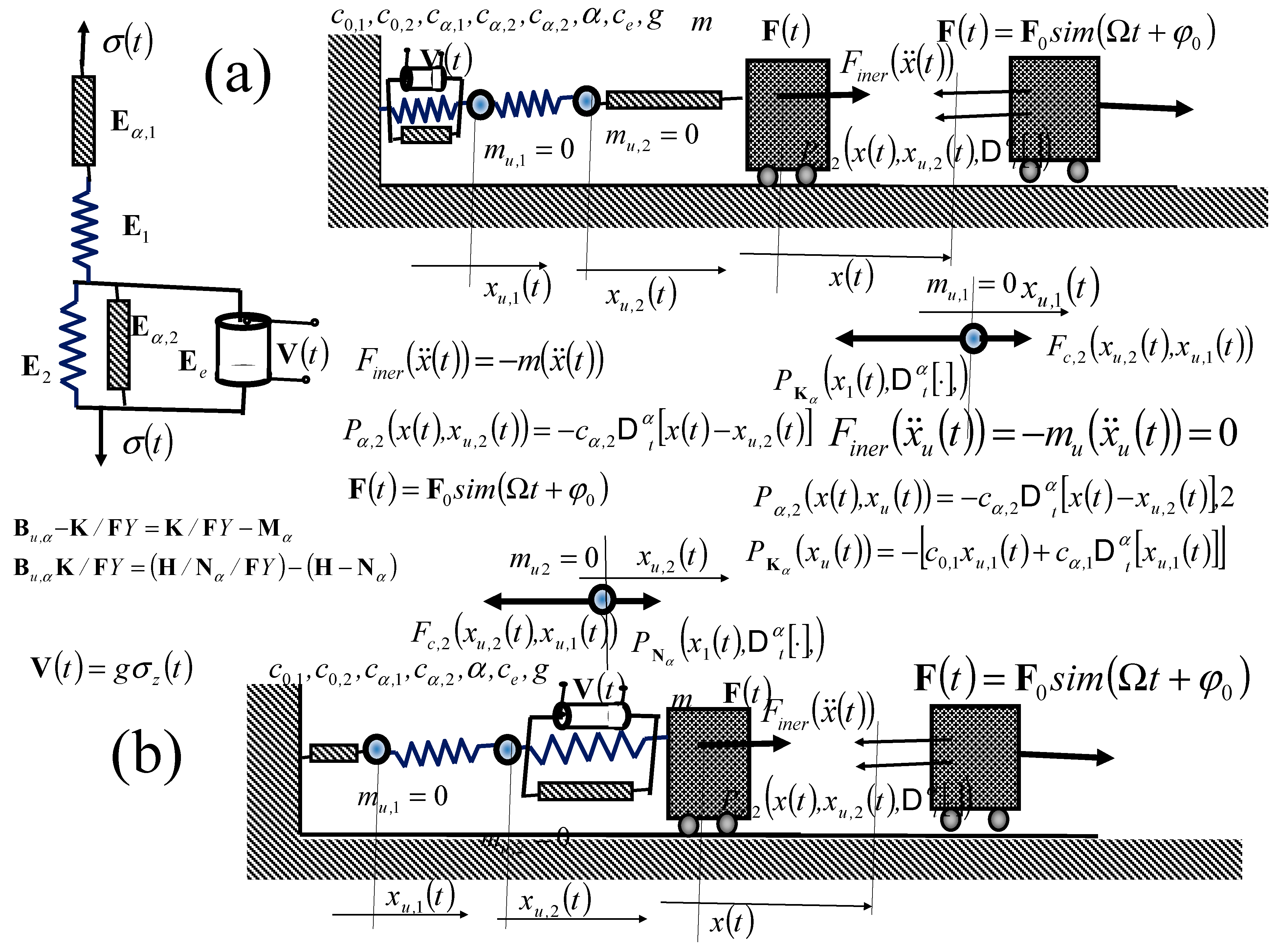
Figure 5.
Burgers–Faraday fractional-type dynamical system fractional type creeper with piezoelectric properties—BFY CF DS. (a) A rheological discrete dynamic system consisting of a single material point (rigid body) with mass , connected by a standard light complex Burgers–Faraday–VF rheological model of the ideal fractional type (BFY CF DS), presented in upper part. The system has one external and two internal degrees of freedom. (b) A dynamic rheological system with the reversed sequence of the structure’s connections in the standard light complex ideal Burgers–Faraday–VF model of fractional type (BFY CF DSR), presented in lower part of (b).
4.1. The Burgers–Faraday (BFY VES DS) Rheologic Discrete Dynamical System of Fractional Type—BFY VES DS Fractional Type Oscillator with Piezoelectric Properties
In this section, we will analyze the dynamics of the complex Burgers–Faraday–VES dynamical system of fractional type in two cases depending on the sequence of elements in the dynamical system. BFY VES fractional-type discrete dynamical systems are presented in Figure 4. Both rheological Burgers–Faraday–BFY VF DS dynamic systems are shown in Figure 4. Let us denote by the independent generalized coordinate corresponding to the external degree of freedom, and and the internal independent generalized coordinates corresponding to the internal degrees of freedom of the ideal fractional-type Burgers–Faraday–VES discrete rheological model.
At the points of serial connections of the simple elements and substructure within the structure of the standard light complex rheological Burgers–Faraday–VES model of fractional type, we place a fictitious material point with zero mass, denoted by and to set up a system of fractional-order differential equations. Given that the basic mass (rigid body) of the system is , and the rheological dynamic Burgers–Faraday–BFY VES DS system (Figure 4a, presented in upper part) has three degrees of freedom, the system of fractional-order differential equations takes the following form:
For the second case of the element connection in the structure of the standard light rheological Burgers–Faraday–(BFY VES DS) model of ideal fractional type, as shown in lower part in Figure 4b, the system of fractional-order differential equations is of the following form:
Let us now introduce the following notations:
Now, let us rewrite the previous systems of the fractional-order differential equations in the following forms:
For the first model of the discrete rheological Burgers–Faraday–VES discrete dynamic system, shown in upper part in Figure 4a (BFY VES DS), the system of fractional-order differential equations is now in the following form:
For the second model of the rheological Burgers–Faraday–VES discrete dynamic system, shown in lower part in Figure 4b, (BFY VF DSR) the system of fractional-order differential equations is now in the following form:
4.1.1. The Dynamics of the Rheological Burgers–Faraday–VES Dynamic System
Now, let us apply the Laplace transform to the previous system of fractional-order differential Equation (62), which results in the following (see References [38,39,40]):
The previous system (64) represents a non-homogeneous system of algebraic equations in terms of the unknown Laplace transforms of the independent generalized coordinates: one external and two internal and , and can be solved using Cramer’s rule by employing the determinant of the system and other determinants derived from it by replacing the appropriate column with the column of the free terms of the system.
The determinant of the previous system (64) of non-homogeneous algebraic equations is in the following form:
While the other determinants obtained by replacing the appropriate column with the column of the free terms from the system (64) are as follows:
The solution of the system (64) of non-homogeneous algebraic equations in terms of the Laplace transforms of the independent generalized coordinates: one external and two internal and can now be expressed in the following form:
Now, it is necessary to determine the inverse Laplace transforms of the external independent generalized coordinate as well as the inverse Laplace transforms of the internal independent generalized coordinates and to transition to the time domain. Thus, we have the following:
where the system determinant is defined in (65).
It is necessary to determine the invers Laplace transform of external independent generalized coordinate , for free eigen fractional type oscillations and transition into the time domain in the following form:
Then, it is necessary to determine invers Laplace transform of external independent generalized coordinate , for forced fractional type rheological oscillations and transition into the time domain in the following form:
We can then also determine the internal independent generalized coordinates and which correspond to the displacements of the points connecting Hooke’s ideal elastic element and Newton’s ideal viscous element of fractional type, with the parallel-connected with piezoelectric Faraday element in the BFY VES DS dynamical system.
The axial strain (dilation) of the parallel-connected Faraday ideal elastic and piezoelectric element, in the structure of the standard light rheological Burgers–Faraday–BFY VES DS model of fractional type (BFY VES DS) (model shown in the upper part of Figure 4a), is as follows:
The normal stress in the parallel-connected Faraday piezoelectric element in the structure of (BFY VES DS) is as follows:
The electric voltage of the electrical polarization in the parallel-connected Faraday element in the structure of (BFY VES DS) is as follows:
and the dielectric displacements in the parallel-connected Faraday element are as follows:
4.1.2. Dynamics of the Reverse Rheological Burgers–Faraday Discrete Dynamic System (BFY VES DSR)
Let us now consider the dynamics of the reverse rheological Burgers–Faraday–VES discrete dynamic system (BFY VES DSR) (model presented in lower part of Figure 4), which is described by the system (63) of three fractional-order differential equations. For the reverse order of element connections in the structure of the standard light rheological Burgers–Faraday–(BFY VES DSR) model of fractional type, we apply the same procedure as in Section 4.1.1, which we will not repeat here. However, we will present the system of non-homogeneous algebraic equations for the unknown Laplace transformations of the independent generalized coordinates, one external coordinate and two internal independent generalized coordinates and describing the dynamics of the rheological system, in the following form:
Starting from the system of three fractional-order differential Equation (63), and applying the Laplace transformation, we derived a non-homogeneous system of algebraic Equation (77). By applying Cramer’s rule and using the determinants we obtain the solutions for the Laplace transforms of all three independent generalized coordinates, expressed in the following form:
where system determinant is in the following form:
The inverse Laplace transform is performed for all three independent generalized coordinates in order to transfer into the time domain:
The inverse Laplace transform for the external independent generalized coordinate for free eigen rheological oscillations of fractional type is as follows:
Then, using convolution integral and inverse Laplace transform for the following: and , we determine the external independent generalized coordinate , for forced rheological oscillation in time domain in the form:
We can then determine the internal independent generalized coordinates and along with the displacements at the points of sequential connections between the basic Hooke ideal elastic element, the Newton ideal viscous element of fractional type, and the piezoelectric Faraday element in the modified Maxwell rheological fractional-type model which incorporates in parallel piezoelectric properties. This can be expressed via the convolution integral as follows:
The dilation of the parallel connected Faraday ideal elastic and piezoelectric element is as follows:
The normal stress in the Faraday element is as follows:
The electric voltage of electric polarization in parallel connected to the Faraday element is as follows:
And the dielectric displacements in the Faraday element are as follows:
4.2. The Burgers–Faraday Discrete Dynamical System of Fractional Type- Fractional Type Creeper with Piezoelectric Properties—BFY CF DS
In this section, we will examine the dynamics of the rheological Burgers–Faraday– discrete dynamic system, of fractional type with piezoelectric properties, BFY CF DS, as presented in Figure 5. This system will be analyzed in two variations based on the sequence of binding in the underlying structure of the standard light complex rheological Burgers–Faraday–BFY CF DS model (presented in Figure 5). This discrete dynamic system is characterized by a standard light complex rheological Burgers–Faraday–BFY CF DS model of ideal, fractional-type material, integrated into the system through parallel binding with a piezoelectric Faraday ideal elastic element and a Kelvin–Voigt structure of fractional type. This rheological discrete dynamic system exhibits both delayed elasticity and normal stress relaxation properties, under specific conditions of constant normal stress or constant axial dilation over time.
Both rheological Burgers–Faraday–BFY CF DS discrete dynamic systems, possess one external degree of freedom related to motion; specifically, the sliding material point (rigid body) and two internal degrees of freedom associated with movement: sliding and flowing of the fractional type. This behavior is inherent within the complex standard light rheological Burgers–Faraday–VF model.
We will establish that, in both cases, it represents a type of fractional order crawler with energy dissipation within the discrete dynamic system.
Let us denote as the independent generalized coordinate corresponding to the external degree of freedom related to motion; specifically, sliding while and represent the internal independent generalized coordinates corresponding to the internal degrees of freedom associated with sliding motion in the fractional-type rheological Burgers–Faraday–VF model.
At the internal connections of the simple elements within the structure of the standard light complex rheological Burgers–Faraday–BFY CF DS model of fractional type, we introduce a fictitious material point with zero mass at each joint, denoted as and . We then formulate a system of fractional-order differential equations. Given that the basic mass (rigid body) of the system is and the rheological dynamic BFY CF DS system (as shown in the upper part of Figure 5a) has three degrees of freedom for movement, the resulting system of fractional-order differential equations can be expressed in the following form:
Now, let us introduce the following notations:
We can then rewrite the previous systems of fractional order differential equations in the following forms:
For the (BFY CF DS) dynamical system, the system of fractional differential equations is now represented as follows:
For the (BFY CF DSR) dynamical system, the system of fractional order differential equations is now expressed as follows:
4.2.1. Dynamics of the Burgers–Faraday Dynamic System–(BFY CF DS)
By applying the identical procedure as described in detail in Section 4.1.1, we use the Laplace transform on the previous system of fractional order differential Equation (90) to obtain a system of non-homogeneous algebraic equations for the unknown Laplace transformations of the independent generalized coordinates. We solve these equations using Cramer’s rule, utilizing the determinant of the system and other relevant determinants; subsequently, we determine the inverse Laplace transforms for all three independent generalized coordinates, transitioning to the time domain, yielding the following:
where the system determinant is in the following form:
First, it is necessary to determine inverse Laplace transform of the external independent coordinate for eigen free sliding-flow , of fractional type with piezoelectric and transition to the time domain in the following form:
Next, it is necessary to determine the inverse Laplace transformation of the external independent generalized coordinate for forced sliding-flow movements of fractional type with piezoelectric properties, or pulsing under the influence of an external periodic one frequency force, and transition to the time domain in the following form:
The preceding expression (97) is derived based on the convolution integral and the individual inverse Laplace transformations of the expressions: and .
For eigen creeping of the intrinsic points and of the internal structure of the standard BFY CF DS we obtain the following expressions:
For force creeping, and of the internal structure of the standard BFY VF DS, we obtain the following expressions:
Using the convolution integral and the property of three functions , , and in convolution, the Laplace transform can be expressed by multiplying of the Laplace transforms of these two functions , i.e., and .
The axial dilatation of the Faraday element connected in parallel in the BFY VF DS discrete dynamical system is as follows:
The expression for normal stress in the Faraday element connected in parallel in the BFY VF DS discrete dynamical system is equivalent (formally same as) to Equation (85). The electric voltage of the electric polarization in the Faraday element in BFY DS2 is equivalent (formally same as) to Equation (86). And, the dielectric displacements in the Faraday element in the BFY DS2 dynamical system are equivalent (formally same as) to Equation (87).
4.2.2. Dynamics of the Rheological Reverse Burgers–Faraday–CF Dynamic System—BFY CF DSR Crawler
For studying the dynamical behavior for the reverse Burgers–Faraday fractional type system—BFY CF DSR (shown in the lower part of Figure 5b) we applied an identical procedure as described in detail in Section 4.1.1 and Section 4.1.2: we use the Laplace transform on the previous system of fractional differential Equation (91) to obtain a system of non-homogeneous algebraic equations for the unknown Laplace transforms of the independent generalized coordinates. We solve these equations using Cramer’s rule, utilizing the determinant of the system and other relevant determinants; subsequently, we determine the inverse Laplace transforms for all three independent generalized coordinates, transitioning to the time domain, yielding the following:
where system determinant is in the following form:
First, it is necessary to determine the inverse Laplace-transform of the external independent coordinate for eigen free sliding-flow , and transition to the time domain in the following form:
Next, it is necessary to determine the external independent generalized coordinate for forced sliding-flow movements of fractional type under the influence of an external periodic one frequency force by using the integral of convolution and the inverse Laplace transformation of the expressions and in the form:
Also, it is possible to determine the internal independent generalized coordinates of the BFY VF DSR dynamical system:
For forced creeping, and in the BFY CF DSR dynamical system we obtain:
The axial dilatation of the Faraday element connected in parallel in BFY CF DSR discrete dynamical system is as follows:
Normal stress in the Faraday element in BFY VF DSR discrete dynamical system is as follows:
The electric voltage of polarization in the Faraday element in BFY CF DSR discrete dynamical system is as follows:
5. Numerical Analysis
After conducting extensive numerical experiments on the obtained solutions of Laplace transforms , , and for all three independent generalized coordinates , , and of the rheological Burgers–Faraday dynamical systems of fractional type (Figure 4 and Figure 5): BFY VES DS, BFY VES DSR, BFY CF DS, and BFY CF DSR for free and forced movements, we selected only a few characteristic graphs from a multitude of results to present in this work. The Burgers–Faraday–VES rheological models of fractional type are both rheological oscillators of fractional type. The order of binding of the structural elements in the Burgers–Faraday–VES model significantly influences the rheological oscillatory dynamics of the rheological discrete dynamic systems.
In contrast, the Burgers–Faraday–CF discrete dynamic systems represent crawlers with flow behavior, also of fractional type. The dynamics of these two models (BFY CF DS and BFY CF DSR) differ significantly, as the order in which the structural elements are connected in the standard light complex rheological Burgers–Faraday model profoundly influences the system.
We will present the characteristic Laplace transformations of independent generalized coordinate surfaces for the dynamics of rheological discrete dynamic systems (Burgers–Faraday–VES DS and DSR, and Burgers–Faraday–CF DS and DSR). These surfaces will be visualized in coordinate systems defined by the following axes: the elongation of the Laplace transform, the exponent of the fractional-order differentiation operator within the interval , and the parameter of the Laplace transform.
This allows for the formation of a series of sets of Laplace transforms of eigen and forced modes of rheological oscillation dynamics of a rheological Burgers–Faraday–VES DS discrete dynamics system of fractional type.
The set of Laplace transforms and of the eigen modes of independent generalized coordinate of external degree of freedom, of dynamics of (BFY CF DS) presented in upper part of Figure 4, is as follows:
where determinant of the system is in the following form:
The set of Laplace transforms and of the forced modes of independent generalized coordinate of external degree of freedom of dynamics of the rheological Burgers–Faraday–(BFY CF DS) discrete rheological oscillator presented in upper part of Figure 4, is as follows:
The set of Laplace transforms and of the eigen modes of independent generalized coordinate of the internal degree of freedom, of the dynamics of the rheological Burgers–Faraday–(BFY VF DS) discrete rheological oscillatory dynamic system, fractional type with piezoelectric property, presented in upper part of Figure 4, is as follows:
The set of Laplace transforms and of the eigen modes of independent generalized coordinate of the internal degree of freedom, of dynamics of the rheological Burgers–Faraday–(BFY CF DS) discrete rheological oscillatory dynamic system, fractional type with piezoelectric property, presented in upper part of Figure 5, is as follows:
This allows the formation of a series of sets of Laplace transforms of eigen modes and forced modes of crawler-creep dynamics of a rheological Burgers–Faraday–(BFY CF DS) rheological crawler-creep rheological discrete dynamics system, fractional type with piezoelectric property.
The set of Laplace transforms and of the eigen modes of independent generalized coordinate of external degree of freedom, of dynamics of the rheological Burgers–Faraday–(BFY CF DS) discrete rheological crawler-creep discrete dynamic system, fractional type with piezoelectric property, presented in upper part of Figure 5, is as follows:
where determinant determined by expression in the following form:
The set of Laplace transforms and of the forced modes of independent generalized coordinate of the external degree of freedom of dynamics of the rheological Burgers–Faraday–(BFY CF DS) discrete rheological crawler-creep dynamic system, fractional type with piezoelectric property, presented in upper part of Figure 5, is as follows:
The set of Laplace transforms and of the eigen modes of independent generalized coordinate of the internal degree of freedom, of dynamics of the rheological Burgers–Faraday–(BFY CF DS) discrete rheological crawler-creep dynamic system, fractional type with piezoelectric property, presented in upper part of Figure 5, is as follows:
The set of Laplace transforms and of the forced modes of independent generalized coordinate of the internal degree of freedom, of dynamics of the rheological Burgers–Faraday–(BFY CF DS) rheological crawler-creep discrete dynamic system, fractional type with piezoelectric property, presented in upper part of Figure 5, is as follows:
The set of Laplace transforms and of the eigen modes of independent generalized coordinate of the internal degree of freedom, of dynamics of the rheological Burgers–Faraday–(BFY CF DS) discrete rheological crawler-creep dynamic system, fractional type with piezoelectric property, presented in upper part of Figure 5, is as follows:
Figure 6, Figure 7 and Figure 8 show the spatial surfaces of Laplace transforms and eigenmodes of sine-like and cosine-like type, as well as the Laplace transformation of forced mode of the independent generalized coordinate of the external degree of freedom of movement of the rheological Burgers–Faraday–CF DS discrete dynamic system of fractional type with piezoelectric property, crawler type, in the cases of single-frequency periodic force action, presented in the Laplace transformation space and in coordinate system with coordinate axes: elongation of Laplace transformation, the differentiation exponent of the fractional order in the interval , and the Laplace transforms parameter , drawn using analytical Expressions (121), (122) and (124), for different system parameter values.
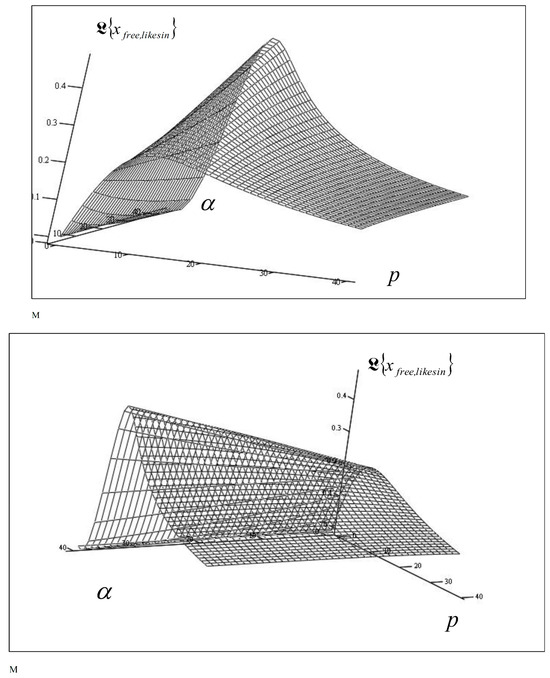
Figure 6.
The space surfaces of the Laplace transform , of the free creep (flow) mode, sine-like type, of the external generalized coordinate of the rheological Burgers–Faraday–VF DS discrete dynamic system of fractional type with piezoelectric property, presented in the Laplace transformation space and in coordinate system with coordinate axes: elongation of Laplace transformation, the differentiation exponent of the fractional order in the interval , and the Laplace transforms parameter , drawn using analytical Expression (121), for different system parameter value.

Figure 7.
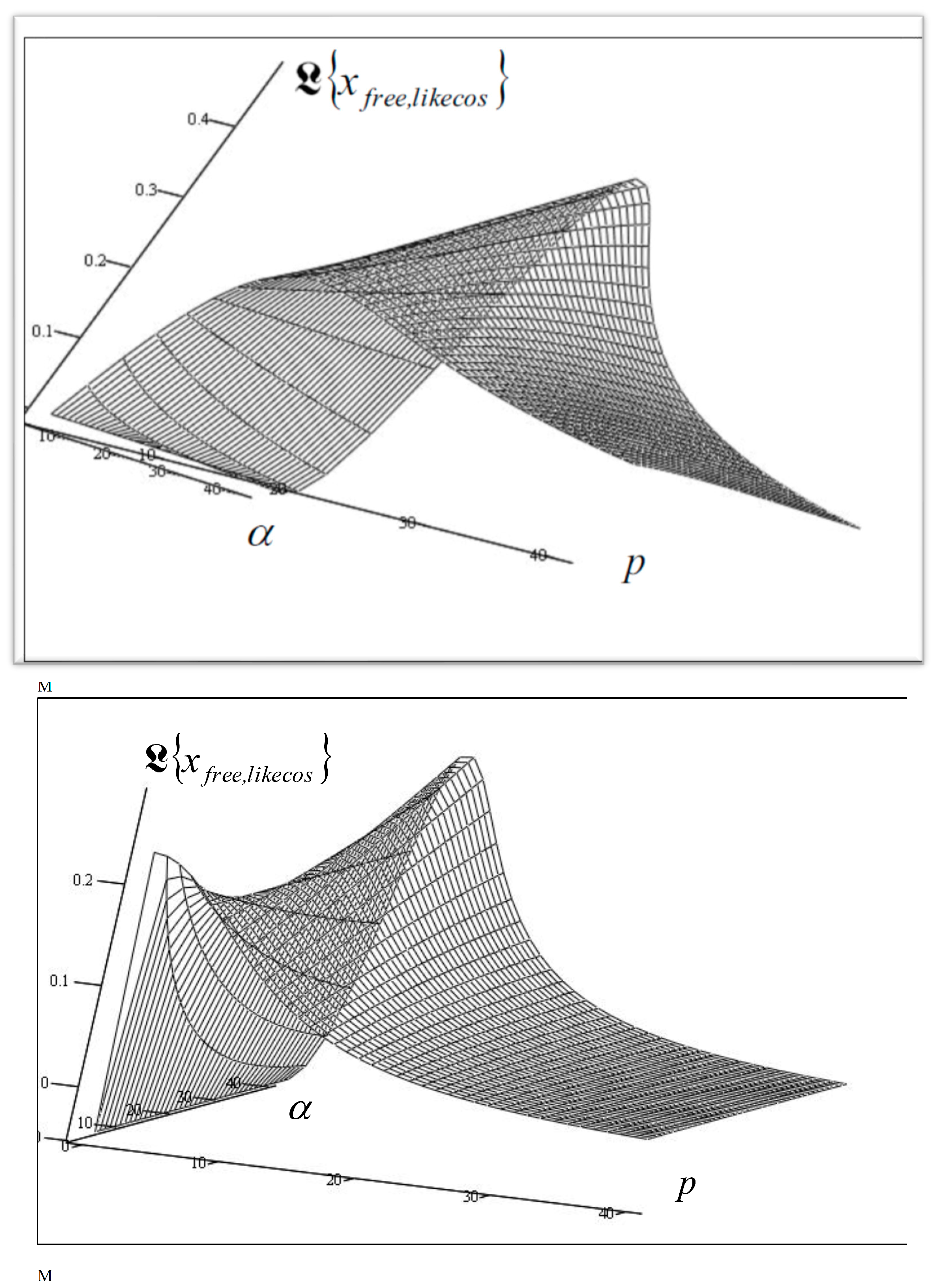
The space surfaces of the Laplace transform , of the free creep (flow) mode, cosine-like type, of the external generalized coordinate of the rheological Burgers–Faraday–VF DS discrete dynamic system of fractional type with piezoelectric property, presented in the Laplace transformation space and in coordinate system with coordinate axes: elongation of Laplace transformation, the differentiation exponent of the fractional order in the interval , and the Laplace transforms parameter , drawn using analytical Expression (122), for different system parameter value.
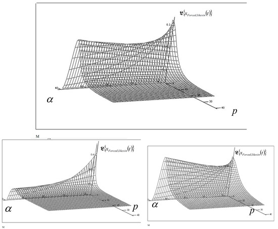
Figure 8.
The space surfaces of the Laplace transform , of the forced creep (flow) mode of the external generalized coordinate of the rheological Burgers–Faraday–VF DS discrete dynamic system of fractional type with piezoelectric property, in the cases of single-frequency periodic force action , presented in the Laplace transformation space and in coordinate system with coordinate axes: elongation of Laplace transformation, the differentiation exponent of the fractional order in the interval , and the Laplace transforms parameter , drawn using analytical expression (124), for different system parameter value.
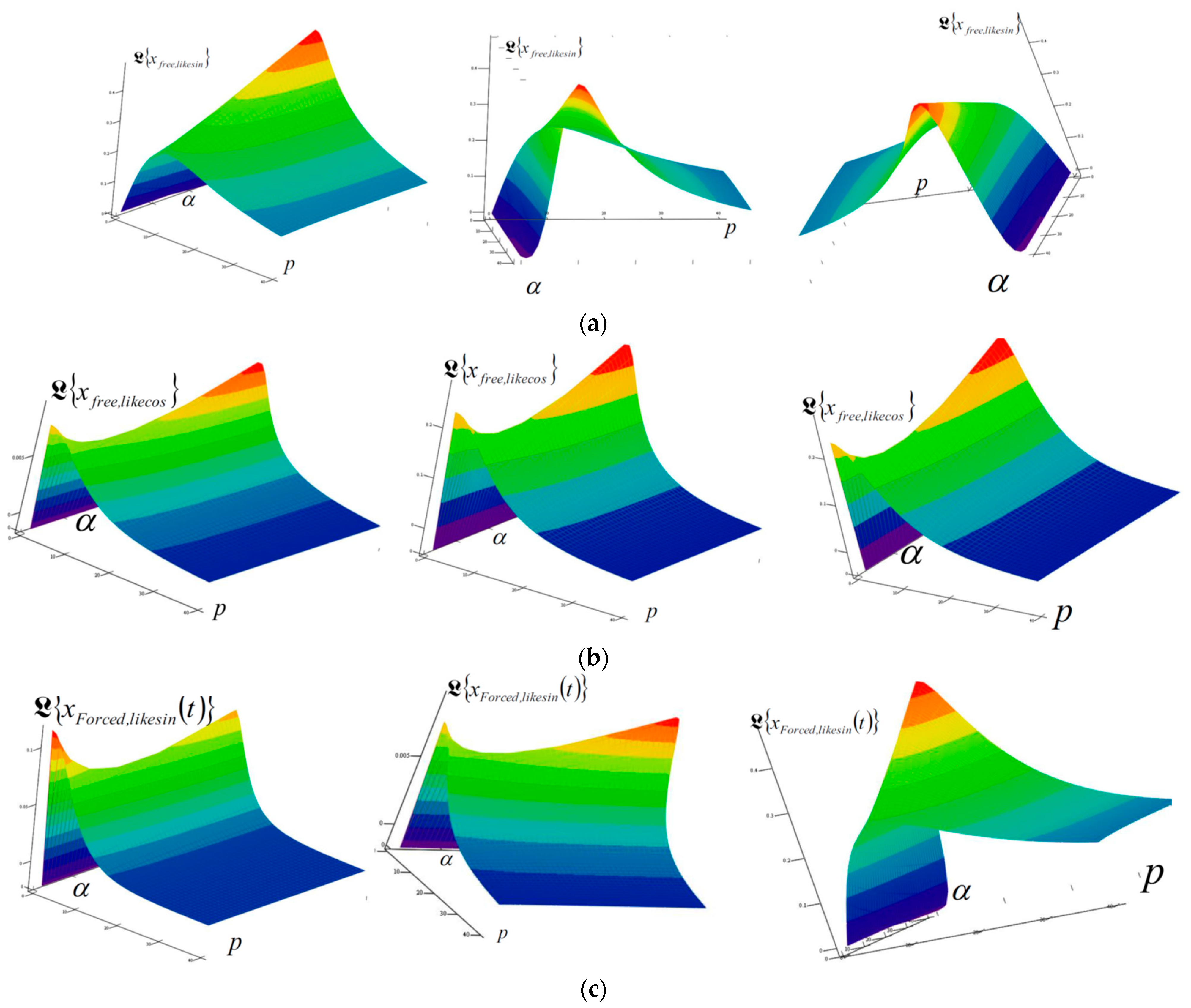
The space surfaces of the Laplace transforms and of the free creep (flow) modes and , of the forced creep (flow) mode of the external generalized coordinate of the rheological Burgers–Faraday–BFY CF DS discrete dynamic system of fractional type with piezoelectric property, in the cases of single-frequency periodic force action , for different system parameter values, presented in the Laplace transformation space drawn using analytical Expression (124), for different system parameter value is shown in the Figure 9.

Figure 9.
The space surfaces of the Laplace transforms and of the free creep (flow) modes and , of the forced creep (flow) mode of the external generalized coordinate of the rheological Burgers–Faraday–BFY CF DS discrete dynamic system of fractional type with piezoelectric property, in the cases of single-frequency periodic force action , for different system parameter values, presented in the Laplace transformation space and in coordinate system with coordinate axes: elongation of Laplace transformation, the differentiation exponent of the fractional order in the interval , and the Laplace transforms parameter , drawn using analytical Expression (124), for different system parameter value. (a) The space surfaces of the Laplace transform , of the free creep (flow) mode, sine-like type, of the external generalized coordinate of the rheological Burgers–Faraday–BFY CF DS discrete dynamic system of fractional type with piezoelectric property, for different system parameter values. (b) The space surfaces of the Laplace transform , of the free creep (flow) mode, cosine-like type, of the external generalized coordinate of the rheological Burgers–Faraday–BFY CF DS discrete dynamic system of fractional type with piezoelectric property, for different system parameter values. (c) The space surfaces of the Laplace transform , of the forced creep (flow) mode of the external generalized coordinate of the rheological Burgers–Faraday–BFY CF DS discrete dynamic system of fractional type with piezoelectric property, in the cases of single-frequency periodic force action , for different system parameter values.
6. Discussion
The development of highly efficient engineering and biomaterials with exceptional viscoelastic, fractional, and piezoelectric properties is a challenge in modern materials science. In this study, we introduce novel Burgers–Faraday models designed to characterize the dynamic behavior of fractional-type materials with coupled fields; specifically, the interplay between mechanical stress and strain and the electric polarization field, facilitated by the Faraday element.
These fractional models, integrating piezoelectric properties, offer analysis of complex systems, such as rheological oscillators and creeping materials.
Based on analytical results and their analysis, we define a number of conclusions here in the form of Theorems:
Theorem 1.
From the structural scheme of the standard light rheological complex model, a distinction can be observed between rheological oscillators and rheological sliders (creeper, crawler) of fractional type, which represent the connections within the rheological discrete dynamic system.
Theorem 2.
If at least one of the Newton viscous fluid elements of fractional type is connected in series within the structure and is not in parallel connection or within parallel connection with any of the Hook ideal elastic elements or Faraday ideal elastic and piezoelectric element, then it is the case of dynamics of the sliding (crawling) elements of the rheological dynamic system.
Theorem 3.
If each of the Newton viscous fluid elements of fractional type is connected in parallel or within a parallel connection with some of the Hook ideal elastic elements or Faraday ideal elastic and piezoelectric elements, then it presents a rheological dynamic system with elastoviscous damped oscillations of fractional type.
Theorem 4.
Every series connection of any of the Newton fluid elements of fractional type introduces one internal degree of freedom of motion for the rheological complex element, in addition to the external degrees of freedom of motion of the complex rheological discrete dynamic system.
Theorem 5.
By comparing the obtained analytical expressions of Laplace transforms for both the free and forced motions of the material point (rigid body in translation), we observed that the order of binding in the standard light structure of the rheological complex Burgers-Faraday-VES discrete dynamic model, DS and DSR, significantly affects the differences in dynamics, but does not change the type of rheological oscillatory dynamics, which remains of fractional and piezoelectric type.
Theorem 6.
By comparing the obtained analytical expressions of Laplace transforms for both the free and forced motions of the material point (rigid body in translation), we observe that the order of binding in the standard light structure of the complex Burgers–Faraday–VF dynamic model DS and DSR significantly affects the differences in creeping-flow dynamics, but does not change the type of creeping-flow dynamics, which remains of fractional and piezoelectric type.
7. Concluding Remarks
In this paper, two rheological models of fractional type with piezo-electrical properties are presented. The models can be applied in modeling viscoelastic and elasto-viscous biomaterials with properties of normal stress relaxation and materials where axial dilation lags behind normal stress and serves as the foundation for the construction of more complex structures of ideal biomaterials, with programmed normal stress relaxation properties and subsequent elasticity. These models are suitable for studying the behavior of complex systems such as rheological oscillators or creepers. Complex models have properties related to the occurrence of internal degrees of freedom that must be taken into account when studying rheological oscillators with piezo-electrical properties of a fractional type. We established fundamental principles and opened a broad field for further research into the properties of rheological discrete and continuously dynamic systems, with many degrees of freedom of movement, both in discrete and continuous systems of fractional type with coupled mechanical and piezoelectric fields.
The proposed models are suitable for advanced material design and the verification of modeling hypotheses, enabling the development of next-generation materials whose performance characteristics hinge on their viscoelastic, elastoviscous, or piezoelectric behavior.
In conclusion, we determined the differential constitutive relations of the fractional order, then gave solutions for the cases of basic complex and hybrid complex models of materials; we defined a class of rheological discrete dynamic systems of fractional type and piezoelectric properties and derived the corresponding systems of differential equations of fractional order, which describe the dynamics of these dynamic systems. Then, we determined the Laplace transforms of the corresponding external and internal independent generalized coordinates.
Complex behavior of materials like bones and cartilage that have both mechanical and piezoelectric properties can be described by the models that are presented in the paper.
Our research addresses a highly relevant area of study and demonstrates significant scientific innovation, offering new insights into the field of material dynamics.
We hope that our new Burgers–Faraday models will inspire other researchers to study the complex dynamics of more complex dynamical systems that can be created on the basis of systems that are studied in this paper.
Author Contributions
Conceptualization, K.R.H. and A.N.H.; methodology, K.R.H.; validation, K.R.H.; formal analysis, K.R.H.; writing—original draft preparation K.R.H. and A.N.H.; writing—review and editing K.R.H. and A.N.H.; visualization K.R.H. and A.N.H. All authors have read and agreed to the published version of the manuscript.
Funding
This research received no external funding.
Institutional Review Board Statement
Not applicable.
Informed Consent Statement
Not applicable.
Data Availability Statement
Data sharing is not applicable. Data are contained within the article.
Acknowledgments
The authors gratefully acknowledge support provided by the Ministry of Science, Technological Development, and Innovation of Republic of Serbia trough Mathematical Institute of Serbian Academy of Sciences and Arts. Authors would like to thank the reviewers for useful comments and suggestions that help in improving the quality of the manuscript.
Conflicts of Interest
The authors declare no conflicts of interest.
Abbreviations
| axial dilatation | |
| normal stress | |
| (SLS) | Standard Linear Solid model |
| Electric voltage in the Faraday element that is generated as a result of polarization closed by mechanical loading in the Faraday element | |
| (KVFYF) | Kelvin–Voigt–Faraday fractional-type model |
| (MFYF) | Maxwell–Faraday fractional-type model |
| the differential operator of fractional order of Caputo type | |
| exponent of fractional order differentiation | |
| the independent generalized coordinate corresponding to the external degree of freedom, | |
| the internal independent generalized coordinate | |
| BFY VF DS | Burgers–Faraday rheologic discrete dynamical system of fractional type with piezelectric property, viscous fluid |
| BFY VF DSR | Reverse Burgers–Faraday rheologic discrete dynamical system of fractional type with piezoelectric property, viscous fluid |
| BFY CF DS | Burgers–Faraday discrete dynamical system of fractional type creeper with piezoelectric properties |
| BFY CF DSR | Reverse Burgers–Faraday rheologic crawler (creeper) of fractional type with piezoelectric properties |
References
- Hedrih, K.; Perić, L.; Mančić, D.; Radmanović, M. Cross Polarized and Electrode Coated Rectangular Pie-zoceramic Plate Strain Problem. J. Electrotech. Math. Fac. Tech. Sci. Kos. Mitrovica 2003, 8, 39–54. [Google Scholar]
- Perić, L. Prostorna Analiza Stanja Napona i Stanja Deformacije Napregntog Piezokeramičkog Materijala (Space Analysis of Stress and Straon State of Stressed Piezoceramiv Materials) [In Serbian]. Master’s Thesis, Faculty of Mechanical Engineering in Niš, Niš, Serbia, 2004. [Google Scholar]
- Hedrih, K.; Perić, L. Method of spatial analysis of piezoelectric body with crack using function of complex variable and computer programming in MATLAB. Int. J. Nonlinear Sci. Num. Simul. 2003, 3, 511–532. [Google Scholar]
- Perić, L. Spregnuti tenzori stanja piezoeletričnih materijala (Coupled tensors of the piesoelectric material states). Ph.D. Thesis, Faculty of Mechanical Engineering in Niš, Niš, Serbia, 2005. (In Serbian). [Google Scholar]
- Dabiri, D.; Saadat, M.; Mangal, D.; Jamali, S. Fractional rheology-informed neural networks for data-driven identification of viscoelastic constitutive models. Rheol. Acta 2023, 62, 557–568. [Google Scholar] [CrossRef]
- Tomović, Z. Reološki model puzanja matriksa meke stijene (Rheologica model of the soft rocks creep). Mater. I Konstr. 2007, 50, 3–19. [Google Scholar]
- Mihailović, V.; Landović, A. The relation properties of concrete and their characteristic in rheological models. Zb. Rad. 2010, 19, 115–124. [Google Scholar]
- Stoiljkoic, D.T.; Petrović, V.; Đurović-Petrović, M. Rheological modeling of yarn elongation. Tekstil 2007, 56, 554–561. [Google Scholar]
- Verdier, C. Rheological Properties of Living Materials. From Cells to Tissues. J. Theor. Med. 2003, 5, 67–91. [Google Scholar] [CrossRef]
- Hedrih, K.R.; Hedrih, A.N. The Kelvin–Voigt visco-elastic model involving a fractional-order time derivative for modelling torsional oscillations of a complex discrete biodynamical system. Acta Mech. 2023, 234, 1923–1942. [Google Scholar] [CrossRef] [PubMed]
- Bonfanti, A.; Fouchard, J.; Khalilgharibi, N.; Charras, G.; Kabla, A. A unified rheological model for cells and cellularised materials. R. Soc. Open Sci. 2020, 7, 190920. [Google Scholar] [CrossRef] [PubMed]
- Fabrizio, M. Fractional rheological models for thermomechanical systems. Dissipation and free energies. Fract. Calc. Appl. Anal. 2013, 17, 206–223. [Google Scholar] [CrossRef]
- Xu, K.; Chen, L.; Lopes, A.M.; Wang, M.; Wu, R.; Zhu, M. Fractional-Order Zener Model with Temperature-Order Equivalence for Viscoelastic Dampers. Fractal. Fract. 2023, 7, 714. [Google Scholar] [CrossRef]
- Araújo, A.; Soares, C.M.; Herskovits, J.; Pedersen, P. Estimation of piezoelastic and viscoelastic properties in laminated structures. Compos. Struct. 2008, 87, 168–174. [Google Scholar] [CrossRef]
- Zhao, F.; Zhou, B.; Zhu, X.; Wang, H. Constitutive model of piezoelectric/shape memory polymer composite. J. Phys. Conf. Ser. 2024, 2713, 012037. [Google Scholar] [CrossRef]
- Cerquiglini, S.; Cignitti, M.; Marchetti, M.; Salleo, A. On the origin of electrical effects produced by stress in the hard tissues of living organisms. Life Sci. 1967, 6, 2651–2660. [Google Scholar] [CrossRef]
- Reinish, B.G.; Nowick, S.A. Piezoelectric properties of bone as functions of moisture content. Nature 1975, 253, 626–627. [Google Scholar] [CrossRef]
- Kao, F.-C.; Chiu, P.-Y.; Tsai, T.-T.; Lin, Z.-H. The application of nanogenerators and piezoelectricity in osteogenesis. Sci. Technol. Adv. Mater. 2019, 20, 1103–1117. [Google Scholar] [CrossRef]
- Yang, C.; Ji, J.; Lv, Y.; Li, Z.; Luo, D. Application of Piezoelectric Material and Devices in Bone Regeneration. Nanomaterials 2022, 12, 4386. [Google Scholar] [CrossRef]
- Bur, A.J. Measurements of the dynamic piezoelectric properties of bone as a function of temperature and humidity. J. Biomech. 1976, 9, 495–507. [Google Scholar] [CrossRef] [PubMed]
- Shamos, M.H.; Lavine, L.S.; Shamos, M.I. Piezoelectric Effect in Bone. Nature 1963, 197, 81. [Google Scholar] [CrossRef]
- Oladapo, B.I.; Ismail, S.O.; Kayode, J.F.; Omolayo, M. Ikumapayi Piezoelectric effects on bone modeling for enhanced sus-tainability. Mater. Chem. Phys. 2023, 305, 127960. [Google Scholar] [CrossRef]
- Carter, A.; Popowski, K.; Cheng, K.; Greenbaum, A.; Ligler, F.S.; Moatti, A. Enhancement of Bone Regeneration Through the Converse Piezoelectric Effect, A Novel Approach for Applying Mechanical Stimulation. Bioelectricity 2021, 3, 255–271. [Google Scholar] [CrossRef]
- Hedrih, K.R.; Machado, J.T. Discrete fractional order system vibrations. Int. J. Non-Linear Mech. 2015, 73, 2–11. [Google Scholar] [CrossRef]
- Hedrih, K.R.; Milovanović, G.V. Elements of mathematical phenomenology and analogies of electrical and mechanical oscillators of the fractional type with finite number of degrees of freedom of oscillations: Linear and nonlinear modes. Commun. Anal. Mech. 2024, 16, 738–785. [Google Scholar] [CrossRef]
- Suzuki, J.L.; Tuttle, T.G.; Roccabianca, S.; Zayernouri, M. A Data-Driven Memory-Dependent Modeling Framework for Anomalous Rheology: Application to Urinary Bladder Tissue. Fractal Fract. 2021, 5, 223. [Google Scholar] [CrossRef]
- Suzuki, J.L.; Naghibolhosseini, M.; Zayernouri, M.A. General Return-Mapping Framework for Fractional Visco-Elasto-Plasticity. Fractal. Fract. 2022, 6, 715. [Google Scholar] [CrossRef]
- Yu, X.; Yin, Y. Fractal Operators and Convergence Analysis in Fractional Viscoelastic Theory. Fractal. Fract. 2024, 8, 200. [Google Scholar] [CrossRef]
- Fahmy, M.A.; Almehmadi, M.M. Fractional Dual-Phase-Lag Model for Nonlinear Viscoelastic Soft Tissues. Fractal. Fract. 2023, 7, 66. [Google Scholar] [CrossRef]
- Hobiny, A.; Abbas, I. The Effect of Fractional Derivatives on Thermo-Mechanical Interaction in Biological Tissues during Hyperthermia Treatment Using Eigenvalues Approach. Fractal. Fract. 2023, 7, 432. [Google Scholar] [CrossRef]
- Pascual-Francisco, J.B.; Susarrey-Huerta, O.; Farfan-Cabrera, L.I.; Flores-Hernández, R. Creep Properties of a Viscoelastic 3D Printed Sierpinski Carpet-Based Fractal. Fractal. Fract. 2023, 7, 568. [Google Scholar] [CrossRef]
- Li, Q.; Sun, Z. Dynamic Modeling and Response Analysis of Dielectric Elastomer Incorporating Fractional Viscoelasticity and Gent Function. Fractal. Fract. 2023, 7, 786. [Google Scholar] [CrossRef]
- Xu, Y.; Luo, Y.; Luo, X.; Chen, Y.; Liu, W. Fractional-Order Modeling of Piezoelectric Actuators with Coupled Hysteresis and Creep Effects. Fractal. Fract. 2023, 8, 3. [Google Scholar] [CrossRef]
- Goroško, O.A.; Hedrih, K. Analitička Dinamika (Mehanika) Diskretnih Naslednih Sistema, (Analytical Dynamics (Mechanics) of Discrete Hereditary Systems); University of Niš: Niš, Serbian, 2001; p. 426. ISBN 86-7181-054-2. (In Serbian). Available online: https://link.springer.com/chapter/10.1007/978-1-4020-8778-3_26 (accessed on 24 October 2024).
- Hedrih, K.R. Generalized Function of Fractional Order Dissipation of System Energy and Extended Lagrange Differential Lagrange Equation in Matrix Form, Dedicated to 86th Anniversary of Radu Miron’s Birth; Tensor Society: Tokyo, Japan, 2014; Volume 75, pp. 35–51. [Google Scholar]
- Ostoja-Starzewski, M.; Zhang, J. Does a Fractal Microstructure Require a Fractional Viscoelastic Model? Fractal. Fract. 2018, 2, 12. [Google Scholar] [CrossRef]
- Mitrinović, D.S.; Djoković, D.Ž. Special Functions (Specijalne funkcije); Gradjevinska Knjiga: Beograd, Serbia, 1964; p. 267. [Google Scholar]
- Hedrih, R.K. Izabrana Poglavlja Teorije Elastičnosti (Selected Chapters of Theory of Elasticity), Mašinski fakultet u Nišu. 1988, p. 425. Available online: http://elibrary.matf.bg.ac.rs/handle/123456789/3766 (accessed on 24 October 2024).
- Rašković, D. Mehanika III—Dinamika (Mechanics IIII-Dynamics), 4th ed.; Naucna Knjiga. 1972. Available online: http://elibrary.matf.bg.ac.rs/handle/123456789/3777 (accessed on 24 October 2024).
- Rašković, D. Teorija oscilacija (Theory of oscillatins). Book. Naucna knjiga, 1st ed.; 1952. Second Edition. 1965. Available online: http://elibrary.matf.bg.ac.rs/handle/123456789/4754 (accessed on 24 October 2024).


Disclaimer/Publisher’s Note: The statements, opinions and data contained in all publications are solely those of the individual author(s) and contributor(s) and not of MDPI and/or the editor(s). MDPI and/or the editor(s) disclaim responsibility for any injury to people or property resulting from any ideas, methods, instructions or products referred to in the content. |
© 2024 by the authors. Licensee MDPI, Basel, Switzerland. This article is an open access article distributed under the terms and conditions of the Creative Commons Attribution (CC BY) license (https://creativecommons.org/licenses/by/4.0/).